Article

Detection of Outliers in Time Series Power Data Based on Prediction Errors

College of Electronics and Information Engineering, Shanghai University of Electric Power, No. 185, Hucheng Ring Road, Pudong New Area District, Shanghai 201306, China
*
Author to whom correspondence should be addressed.
Energies 2023, 16(2), 582; https://doi.org/10.3390/en16020582
Submission received: 28 November 2022 / Revised: 22 December 2022 / Accepted: 30 December 2022 / Published: 4 January 2023
(This article belongs to the Section K: State-of-the-Art Energy Related Technologies)

Abstract

:
The primary focus of smart grid power analysis is on power load forecasting and data anomaly detection. Efficient and accurate power load prediction and data anomaly detection enable energy companies to develop reasonable production and scheduling plans and reduce waste. Since traditional anomaly detection algorithms are typically for symmetrically distributed time series data, the distribution of energy consumption data features uncertainty. To this end, a time series outlier detection approach based on prediction errors is proposed in this paper, which starts by using an attention mechanism-based convolutional neural network (CNN)-gated recursive unit (GRU) method to obtain the residual between the measured value and its predicted value, and the residual data generally conform to a symmetric distribution. Subsequently, for these residual data, a random forest classification algorithm based on grid search optimization is used to identify outliers in the power consumption data. The model proposed in this paper is applied to both classical and real energy consumption datasets, and the performance is evaluated using different metrics. As shown in the results, the average accuracy of the model is improved by 25.2% and the average precision is improved by 17.2%, with an average recall improvement of 16.4% and an average F1 score improvement of 26.8% compared to the mainstream algorithms.

1. Introduction

Abnormality detection in energy consumption data helps to identify unusual conditions in grid data in time to alert staff who can then conduct an overhaul or maintenance of the grid to ensure continuous operation of the power system. Classic anomaly detection methods are mainly divided into the following categories. (1) Statistic-based outlier anomaly detection: employing statistical principles to identify data with a low probability distribution in the data set as outliers. (2) Clustering-based outlier anomaly detection: performing a cluster analysis on unlabeled data sets by means of grouping. Typically, groups of clusters can be regarded as normal data, and so relatively abnormal data are then compared with the clusters to determine outliers [1]. (3) Classification-based outlier anomaly detection: For data sets with class labels, a classifier is usually trained to distinguish between normal and abnormal data. This method often has specific requirements for samples [2]. (4) Proximity-based outlier anomaly detection: to define the “proximity” between data and then determine outliers based on this value. Typical approaches to proximity-based methods include density-based methods [3], which use neighborhood “density” to reflect proximity, and distance-based methods [3] using the global “distance” to reflect proximity. These approaches have all been widely employed in time series outlier detection; however, there is an issue with these classical methods: The method is effective when the data are symmetrically distributed and significantly correlated, but energy consumption data are not necessarily symmetrically distributed or significantly correlated. To solve such problems, researchers have proposed a combined, residual-based approach for anomaly detection [4]. An energy consumption prediction model is built and the residual series is obtained by comparing the predicted results of this model to the original data. The anomaly detection algorithm is then applied to the residual series to detect outliers. Points with large differences can be considered anomalies.
A combination of regression methods (e.g., random forest) and adjusted box plot anomaly detection methods was used by Gustavo Felipe Martin Nascimento [5] to detect energy consumption data anomalies by applying them to actual measured values and the differences between measured values and their predicted ones. This approach shows promising potential for detecting such power consumption data quality issues. Tianyu Li [6] proposed a prediction-based anomaly scoring method for anomaly detection. Li used a long short-term memory (LSTM) network for prediction and assigned scores to each anomaly based on the distance between each detected anomaly in the test data and the nearest FPS pattern learned from the training data. Nur Shakirah Md Salleh [7] proposed a combination of regression method, least squares model, and mathematical solution instead of the commonly used classification method for anomaly detection, which is used for power load prediction and identifies the point of occurrence of anomalous events by threshold and prediction error values. Using the idea of prediction error compensation, Qixun Zhou [8] introduced a three-vector PTC method based on online prediction error compensation (TVPTC), which stores and updates the errors of all voltage vectors for reliable compensation to enhance parameter robustness. An adaptive control scheme incorporating uncertainty prediction error estimation was developed by Rusong Zhu and Ping Wang [9] for uncertain nonlinear systems with constrained input actuators (including amplitude saturation and rate saturation). This scheme enhances the estimation of uncertainty in the system and brings stability to the parameter estimation error unavailable with conventional adaptive control. Anil K. Madhusudhanan [10] proposed a fuel flow modeling approach for diesel and compressed gas engines based on prediction error identification and road data collection. Road vehicle data are collected during normal transportation operations and the results show that prediction error expansion (PEE) is typically the most effective mechanism for hiding reversible data using redundancy in the cover medium. A coordinated control strategy for complementary scenic energy storage that balances prediction error compensation and fluctuation suppression was proposed by Shuyan Zhang [11]. The statistical probability distribution is used to analyze the prediction error and power fluctuation, and the target region for compensating the prediction error and smoothing fluctuation is established. Based on the upper and lower limits of the allowable prediction error, the charging and discharging reference power of the target area is defined to compensate for the prediction error. The above research results demonstrate the feasibility of the prediction error method in targeting time series anomaly detection.
As residual-based anomaly detection methods require a high accuracy of prediction results, these methods are still not accurate enough and the generalizability of the model is weak regarding different energy consumption data for residual detection methods. Therefore, this study proposes a combined CNN-GRU-ATTENTION and GridSearchCV-RandomForest method for residuals, hereafter referred to as CGA-RF. In this scheme, the first step uses a CNN-GRU-ATTENTION based prediction model in which a CNN can fully extract the feature vectors from energy consumption data [12]. Dynamic changes are then fully modeled by the GRU [13,14], and an attention mechanism is employed to take a probabilistic view of resource allocation, enhancing the selection of important information [15,16,17]. High-precision prediction results are then obtained to compare the difference with the original data to obtain a new sequence of reconstructed residuals. In the second step, a random forest classification and detection algorithm based on grid search is used. The random forest algorithm is composed of multiple mutually independent decision tree classifiers [18], which is an integrated learning method based on a decision tree algorithm where the final classification result is determined by the vote of all decision tree algorithms. Here, the selection of classifier parameters is a particularly important step. In this study, a grid search approach was chosen for parameter optimization [19,20,21], and then applied to the random forest classifier with optimized parameters for anomaly detection in residual sequences. The present research applies three sections of the datasets for validation; the first part is a real-time energy consumption series dataset used to validate the prediction ability of the CNN-GRU-ATTENTION model, the second part is a UCR classical time series classification dataset used to validate the anomaly detection ability of the GridSearchCV-RandomForest model, and the third part is a real data set containing outlier energy consumption data to verify the anomaly detection ability of the combined CGA-RF method chosen for analysis in the present study. Experimental results prove that this new, hybrid method has high detection accuracy of anomalies in energy consumption data.
The rest of the paper is presented as follows: in Section 2, the anomaly detection method based on prediction errors is described. In Section 3, the model is validated using classical and real datasets. In Section 4, the results are analyzed and discussed.

2. Anomaly Detection Method Based on Prediction Error

2.1. Methodology Overview

The CGA-RF method chosen in the present study is divided into two main parts. Firstly, a CNN-GRU model based on a self-attentive mechanism to effectively model the energy consumption data, and the predicted value of electricity consumption at the current moment as obtained from historical data. To generate a new sequence of residuals, the predicted and true values are subtracted to obtain the residuals. The new, reconstructed sequence of residuals is then classified using the random forest algorithm optimized by grid search to detect any outliers in the energy consumption data. The algorithm progression as shown in Figure 1 is described in the following steps.
(1) Raw energy consumption data pre-processing. Obtain raw energy consumption data (time series data) to form data samples and perform normalized pre-processing on all data samples.
(2) Data prediction. The CNN-GRU model based on a self-recognizing mechanism is used to predict energy consumption data moment by moment and the predicted values of each instant are used to generate a new predicted series. Predicted values of corresponding moments are then subtracted from the true values and a new sequence of residuals is obtained.
(3) Anomaly detection. The random forest algorithm optimized by grid search is used to classify and detect a new sequence of residuals and detect outliers.
(4) Evaluation index calculation. The outliers detected by classification are labeled as anomalies and compared with the true labels of the data samples to calculate the corresponding evaluation metrics.

2.2. Predictive Models

2.2.1. CNN-GRU Prediction Model Based on the Attention Mechanism

In the study of load forecasting for electrical energy data, the electrical energy load sequence fluctuates due to random and nonlinear input. These influencing factors are diverse and complex (seasonal changes, temperature, humidity, weather, wind speed, holidays, etc.), which makes accurate forecasting a challenge. Neural networks feature self-learning and self-adaptive capabilities with the ability to deal with complexity and nonlinearity, as well as the capacity to adapt to complex and dynamic systems. These new systems can adequately solve the nonlinear problems that exist in large-scale load data and are therefore more widely used in the field of power load forecasting [22,23].
CNN is a commonly used deep learning algorithm that is widely utilized for text and image recognition. CNNs contain convolutional computation and maintain a deep structure of neural networks that often contain multiple hidden layers between a single input and output layer. These hidden layers are: convolutional, dense, max-pooling, dropout, and flatten [23]. The advantage of this structure is that it effectively reduces the number of structural weights, simplifies the network structure, and reduces complexity. The CNN model of convolutional pooling for historical data feature extraction saves computational time, improves computational efficiency, and models time series data well.
GRU is an updated version of the recurrent neural network (RNN). A GRU network can target the characteristics of load data uncertainty, effectively modeling dynamic time series data. The structure of the GRU has only two primary gates: update gate and reset gate [24]. The role of update gate is intended to regulate how much historical series information needs to be passed forward. It is useful for eliminating the risk arising from gradient descent by remembering historical information and deciding which messages are valid information and which are not. Reset gate is meant to forget some of the invalid information. The feature vector extracted from the CNN is input to the GRU to better learn the periodic change demand pattern in load data. However, the energy consumption data input is excessively long and the GRU network is prone to issues such as missing information and difficulties in modeling.
The attention mechanism is a resource allocation system that assigns different probability weights to the feature vectors input from the GRU layer, mainly to enhance the probability of important information to avoid loss. This, in turn, solves the problem of sequence loss that may occur in the model for load data due to long sequences, improving the model regarding important features in long sequence historical information. The CNN-GRU-ATTENTION model selected for this study uses the CNN model to extract effective feature vectors from load history data, which are then input to the GRU layer for effective modeling. The attention mechanism is employed to avoid the loss of effective information. By combining multiple structures for the effective processing of load data, the accuracy of load prediction is improved.

2.2.2. Model Structure

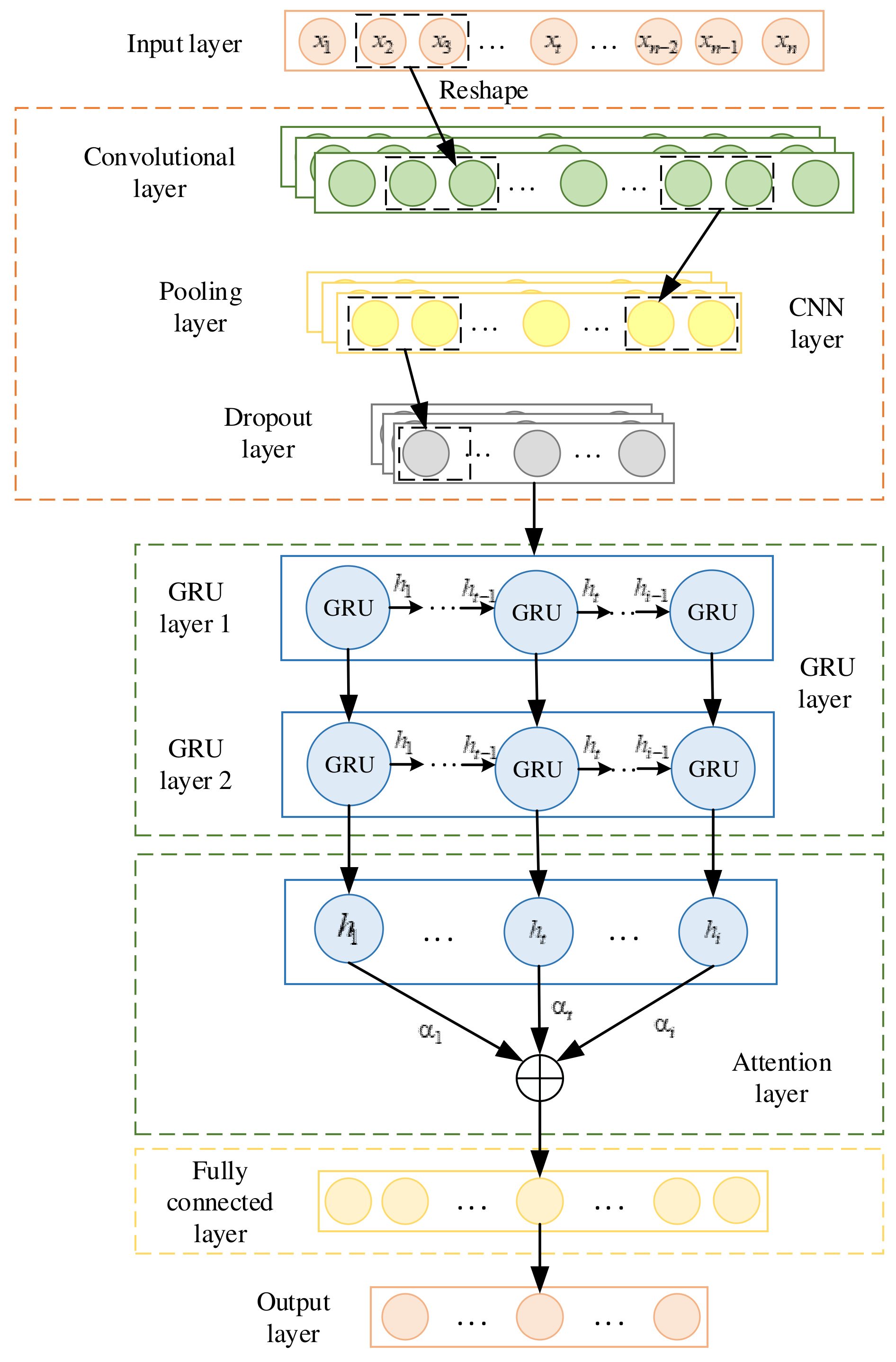
The structure of the CNN-GRU-ATTENTION prediction model proposed in the current study is shown in Figure 2; it is divided into the input layer, convolutional layer, pooling layer, dropout layer, GRU layer, attention layer, fully connected layer, and output layer.
The structure of the CNN-GRU model is based on the attention mechanism input layer. This layer is the beginning of the CNN model, without any weight input. In this stage, historical load data are input into the prediction model with the input vector represented by X.
CNN layer: For the current research, a CNN framework consisting of a convolutional layer, pooling layer and dropout layer was assembled. According to the time series, the convolutional layer is designed as a one-dimensional convolution with the ReLU used for activation. The convolution layer is input with data reshaped from the output of the input layer. The pooling layer uses the maximum pooling method, which is used to retain the maximum historical information of the load. Load data are then mapped to the hidden layer feature space after processing in the convolution layer and pooling layer, and then fed to the dropout layer. The role of the dropout layer is to randomly prevent the weights of certain hidden layer nodes of the network from working temporarily. Those nodes can be temporarily considered not part of the network structure, but their weights must be retained as they may have to function again in the next sample input. The output feature vector H C of the CNN layer can be expressed as:
C 1 = f ( X W 1 + b 1 ) = ReLU ( X W 1 + b 1 )
P 1 = m a x ( C 1 ) + b 2
H C = f ( P 1 × W 2 + b 3 ) = Sigmoid ( P 1 × W 2 + b 3 )
where C 1 is the output of the convolution layer; P 1 is the output of the pooling layer; W 1 is the weight matrix; b 1 , b 2 and b 3 are the bias terms; max() is the maximum function; and the output of the CNN layer is denoted as H C .
GRU layer: The main role of the GRU layer is to fully learn the sequence feature vector of the CNN layer input. The output of the GRU layer is denoted as MISSING, and the output at step t is denoted as H C .
h t = GRU ( H C , t 1 , H C , t ) , t [ 1 , i ]
Attention layer: The output vector of the GRU network layer is the input for the attention layer, and, according to the weight assignment of the self-attentive mechanism, the probabilities of different feature vectors are updated and iterated to calculate an improved weight parameter matrix.
e t = u tan h ( w h t + b )
α t = exp ( e t ) j = 1 t e j
s t = t = 1 i α t h t
where e t denotes the value of the attention probability distribution determined by the GRU layer output vector h t at moment t; u and w are the weight coefficients; b is the bias term; and the output of the attention layer at moment t is s t .
Output layer: The input of the output layer is the result generated by the attention mechanism layer. The mechanism of the output layer is the output of the computation through the fully connected layer. The prediction formula is expressed as follows:
y t = S i g m o i d ( W 0 + b 0 )
where y t denotes the predicted output value at time t; W 0 is the weight matrix; b 0 is the deviation terms; and the ReLU function is the activation function of the dense layer for the present research.

2.3. Detection Models

2.3.1. Random Forest Classification Detection Model

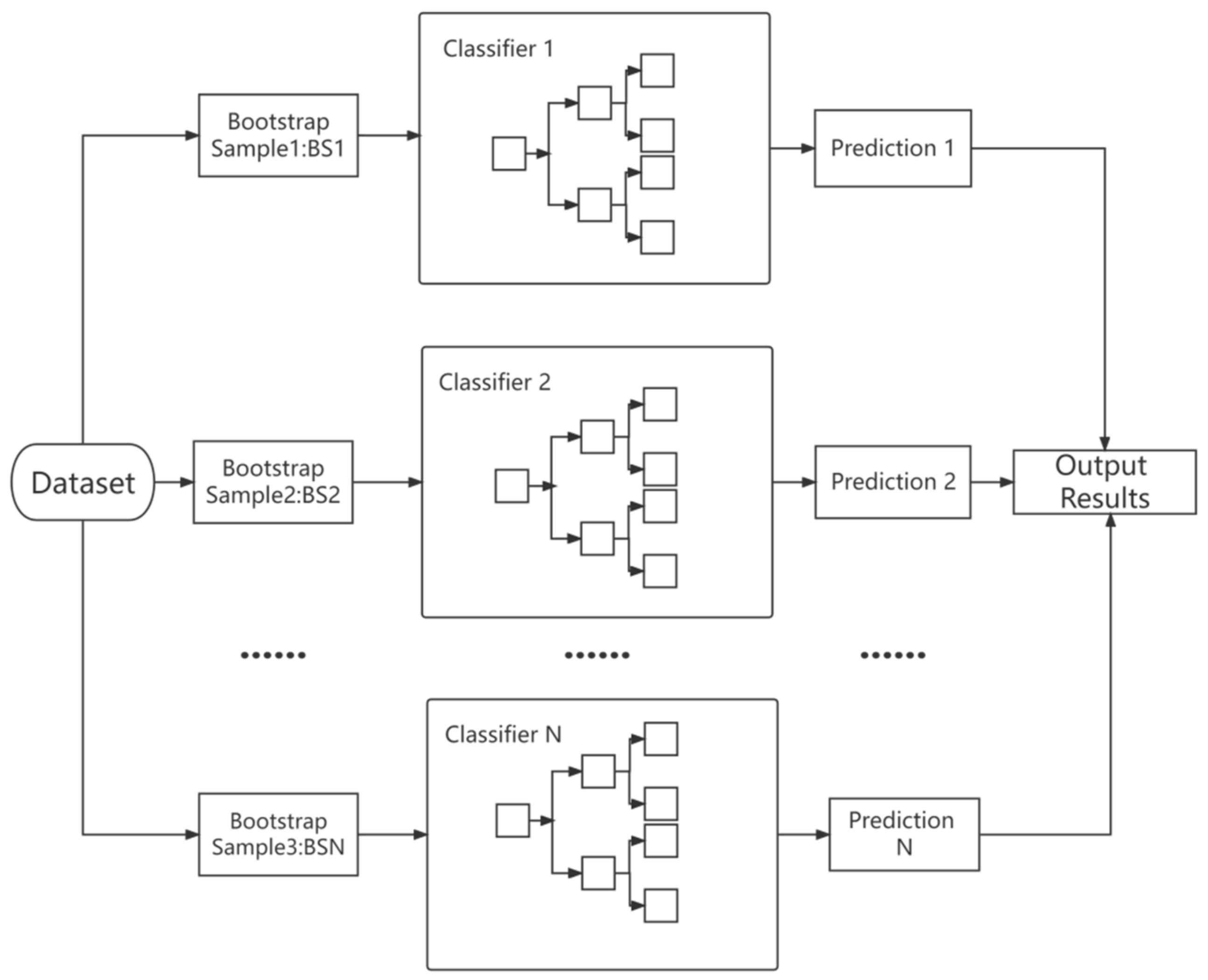
The random forest algorithm is derived from integrated learning theory [25,26,27,28,29,30,31]. The model used in this study combines several independent classifiers. In order to simplify non-parameters and improve computational efficiency, classifiers are usually selected as regression trees to be used in the model algorithm [26]. Each classifier independently bootstraps the dataset randomly. The structure of the classification model is shown in Figure 3. For the classification detection problem, it is first assumed that the training data contain N observations, and in order to reduce errors associated with classification, an overlapping sampling solution called “bagging” is used in the model [27]. Specifically, the algorithm extracts observations by substitution, which, in turn, leads to the generation of independent bootstrap samples in the dataset. Each classifier is then trained from different bootstrap samples, thus increasing the diversity of the tree. To better reduce the correlation between various classifiers, the best splitting scheme for each node is obtained by randomly selecting a subset of M features instead of all M features. As a result, the classifiers within the model can continue to grow without pruning, which in turn reduces the computational burden. Moreover, by using different random samples and node features, the noise immunity of the model can be improved with the help of averaging various de-correlated classifiers [28,29]. In addition, for each classifier in the model, a bagging solution is adopted that utilizes a sampling method with put-back to generate training data. Through multiple rounds of random sampling of the initial training set with put-backs, multiple training sets are generated in parallel, corresponding to multiple base classifiers (without strong dependencies between base classifiers), and then these base classifications are combined to build a strong classifier. The essence of this is the introduction of sample perturbation, which reduces the variance by increasing sample randomness. In this way, the model is able to achieve unbiased estimation without using external subsets of data [30,31].

2.3.2. Optimization of Grid Search Parameters

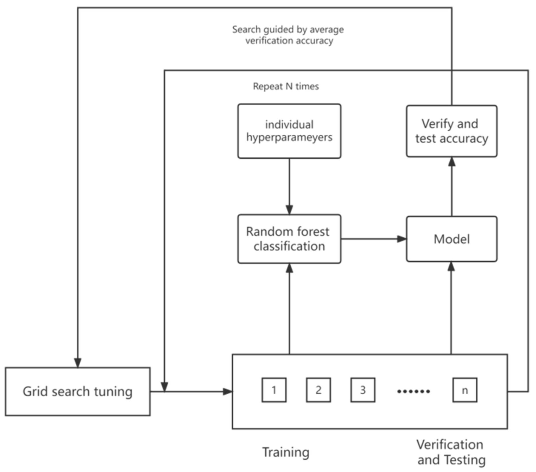
The selection of suitable parameters is the best way to achieve optimal detection. The fine tuning of parameters to obtain optimal model performance is called parameter tuning and a common method of tuning parameters is grid search [32,33], essentially an exhaustive method. The combination of model and hyper-parameters is chosen by exhaustively enumerating all parameter combinations required in the model and comparing, analyzing, and verifying each combination one by one. The purpose of the grid search is to identify the combinations that yield the best model performance, which can then be selected for use as a predictive model. A comparative analysis is performed to obtain an optimal set of hyper-parameters. To understand the origin of the name “grid search” [34], we first assume the existence of two hyper-parameters of the model, while each hyper-parameter has a set of candidate parameters and both sets of parameters are simultaneously parallel. These two sets of candidate parameters can be combined in pairs with all combinations classified as two-dimensional lattices (the case of multiple sets of hyperparameters combined in pairs can be considered lattices in higher dimensional spaces). The model then traverses all nodes in the lattice to select the optimal solution. Therefore, it is called grid search.
The grid search tuning process is shown in Figure 4, where the input data are first partitioned into a training set, a test set, and a validation set. The data set is divided into n parts to perform parameter tuning. Then, the parts of the random forest classification model that need parameter tuning are trained in (n − 2) parts for each alternative. A validation set is used to verify the performance of the model after parameter optimization and, finally, is used to test the model performance. The detection and validation accuracy of the tuned model are evaluated, and then the hyper-parameters are determined from the training set and tuning technique. The above steps are repeated n times and the average validation accuracy is taken as the fitness value. Finally, the highest test accuracy is determined.

2.4. Evaluation Metrics of Prediction and Detection Models

2.4.1. Evaluation Indices of Prediction Models

In order to evaluate the accuracy of the prediction model, the mean absolute error MAE, mean absolute percentage error MAPE, mean square error MSE, root mean square error RMSE, and coefficient of determination R2 (R-squared) were chosen for evaluation criteria, and they are expressed as:
M A E = 1 n i = 1 n | y ^ i y i |
M A P E = 100 % n i = 1 n | y ^ i y i y i |
M S E = 1 n i = 1 n ( y ^ i y i ) 2
R M S E = 1 n i = 1 n ( y ^ i y i ) 2
R 2 = 1 i ( y ^ i y i ) 2 i ( y ¯ i y i ) 2
where X is the total number of prediction results; y i and y ^ i are the actual load value and predicted load value of the ith sampling point of the prediction, respectively. MAE and MAPE can measure the superiority of the prediction model results, and RMSE and MSE can evaluate the accuracy of the prediction, which is sensitive to large or small errors in the results. R2 can describe the quality of the model. Generally, the larger the value of R2, the better the model fit, and the smaller the value of the above evaluation indicator, the more accurate the load prediction result. Smaller values of the above evaluation indices indicate more accurate load forecasting results.

2.4.2. Evaluation Index of Detection Model

Labeling load data as normal or abnormal points is essentially a classification problem. Several methods are used to evaluate the performance of models in solving such problems. In this paper, the concepts of accuracy, precision, recall, and F-score (or F1) are applied. These metrics are defined by the following equations:
A c c u r a c y = TP   +   TN T P + T N + F P + F N
P r e c i s i o n = TP T P + F P
R e c a l l = TP T P + F N
F 1 = 2 × ( Precision   ×   Recall P r e c i s i o n + R e c a l l )
where TP is the number of true positives classified (outliers detected in practice), FP is the number of false positives classified (normal samples mistakenly detected as outliers), FN is the number of false negatives (no outliers detected), and TN is the number of true negatives for classification (error samples are not detected as outliers). In the outlier detection task, the accuracy rate indicates the proportion of points rated as normal by the model in all data. Recall rate indicates the proportion of normal data from all data that were attempted to be detected (resulting in normal data detected as normal and abnormal data detected as abnormal). F1 score is the summed average of the accuracy rate and recall rate.

3. Results and Analysis

3.1. Performance Analysis and Comparison of Load Consumption Data Prediction Models

3.1.1. Comparison of Prediction Results for the Spanish Wind Power Dataset

In this study, a Spanish wind power dataset was used for training and prediction. The training and test subsets were divided in a ratio of 8:2. The parameters of the model are reported in Table 1.
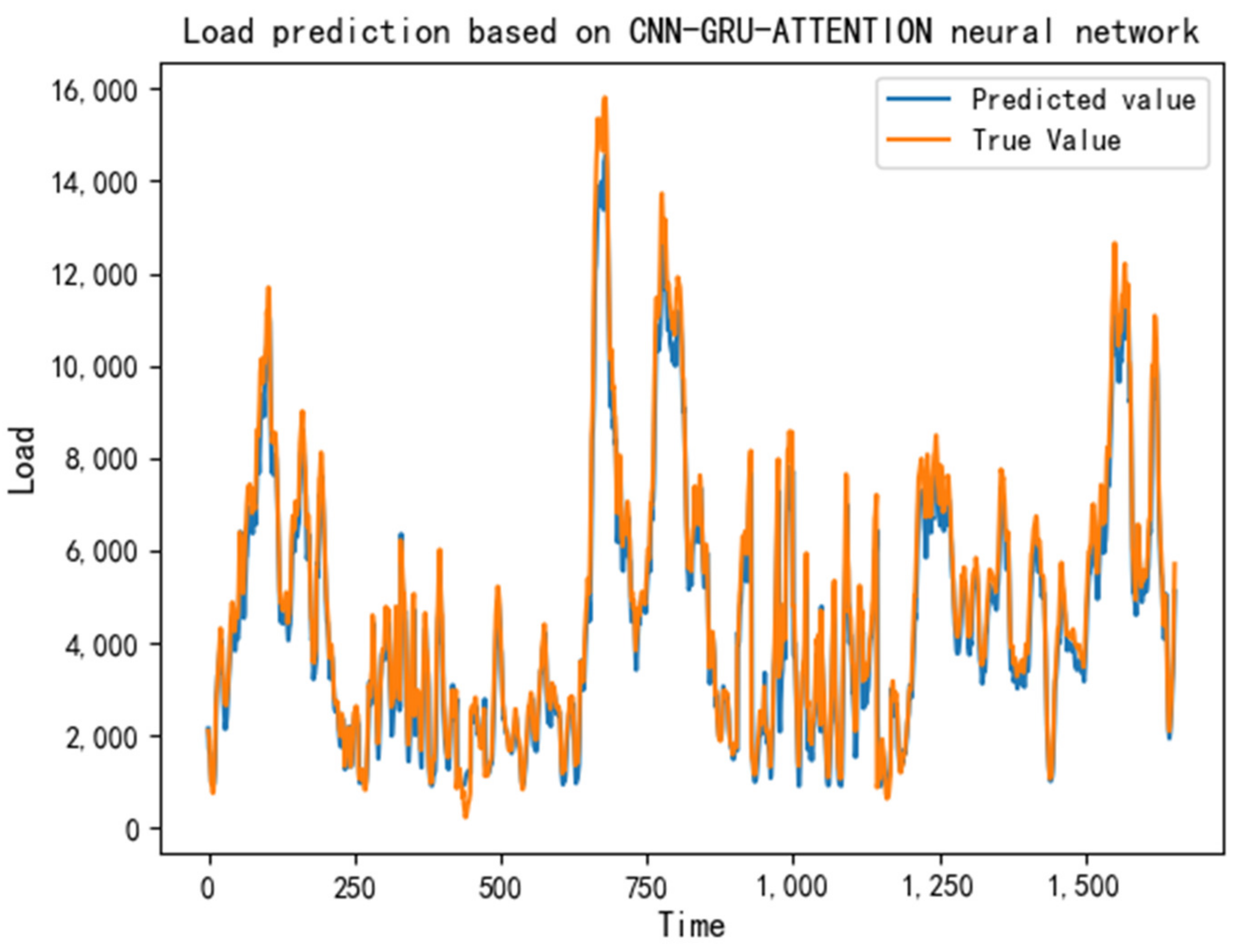
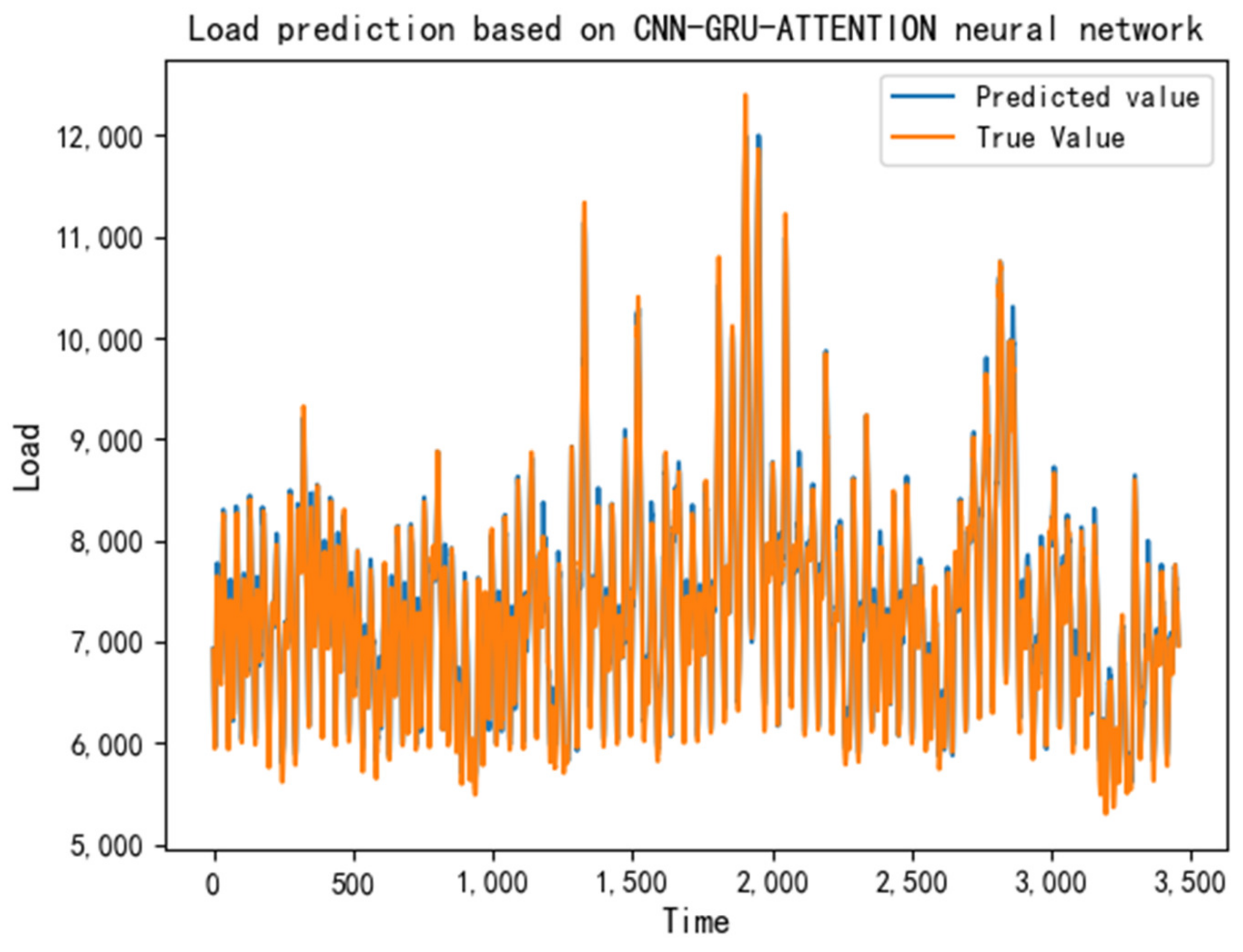
In order to verify the validity and stability of the model, daily load predictions were performed on a test set covering one week per month over six months. The prediction results are shown in Table 2, and a comparison of the predicted and true values is shown in Figure 5.
From each error indicator, it can be seen that the prediction results are accurate to each day, the value of MAPE is relatively low, the prediction error is small, and the prediction accuracy is relatively high. From the analysis of the prediction results for a single day compared with the other three methods, the method used in this study (CNN-GRU-ATTENTION) has the highest prediction accuracy, and the MAPE values are reduced by 3.445%, 10.351%, 3.956%; 1.984%, 2.072%, 0.939%; 1.589%, 1.852%, 1.122%; 0.61%, 0.786%, 0.185%; 1.32%, 0.7%, 0.27%; 1.308%, 1.652%, 0.564%; 2.597%, 1.361%, 0.993%; 1.908%, 2.906%, 2.26%. In the comprehensive analysis, the study’s hybrid method has significantly reduced the MSE, RMSE, MAE, and MAPE indices and generated a significant increase in the R2 index, which indicates that the overall prediction accuracy and model performance have been greatly improved for the prediction process.

3.1.2. Comparison of Forecast Results for the Australian Electricity Price Dataset

For the purpose of this study, the Australian load output dataset was used for training and prediction. As before, the training and test sets were divided in a ratio of 8:2. The parameters of the model are reported in Table 3.
In order to verify the validity and stability of the model, daily load predictions were performed in a test set covering one week per month. Prediction results are shown in Table 4, and a comparison of predicted and true values is shown in Figure 6.
From each error indicator, it can be seen that the prediction results are accurate to each day, the value of MAPE is relatively low, the prediction error is small, and the prediction accuracy is relatively high (1.122%; 0.61%, 0.786%, 0.185%; 1.32%, 0.7%, 0.27%; 1.308%, 1.652%, 0.564%; 2.597%, 1.361%, 0.993%; 1.908%, 2.906%, 2.26%). In a comprehensive analysis, the methods used in this study have significantly reduced MSE, RMSE, MAE, and MAPE indicators, leading to a significant increase in R2 indicators, which shows a significant improvement in the overall prediction accuracy and model performance of the prediction process.

3.2. Performance Analysis and Comparison of Outlier Point Detection Models

This study conducted experiments using the UCR time series classification dataset, which consists of publicly available time series datasets that vary according to the number of samples and the length of the time series. A standard partition is used to divide each dataset into a training set and a test set. For this research, a typical time series classification dataset with different time series lengths for different numbers of classifications was extracted. From the results in the table below, it is shown that the GridSearchCV-RandomForest algorithm selected for this study has significantly improved accuracy, precision, recall, and F1 score compared to other machine learning algorithms.
From Table 5, Table 6, Table 7, Table 8 and Table 9, it is evident that the grid search optimized random forest algorithm utilized in this study is superior for detection than traditional integrated classification algorithms. From the FreezerRegularTrain dataset, it is evident that compared to RandomForest, DecisionTree [35,36,37], and AdaBoost [38] algorithms, GridSearchCV-RandomForest offers significant improvements in accuracy, precision, recall, and F1 score; in the PowerCons dataset, the GridSearchCV-RandomForest algorithm showed 100% accuracy in precision, recall, and F1 score. In the Wafer dataset, the GridSearchCV-RandomForest algorithm detected 620 true anomalies with 2.05% and 23.28% improvements in accuracy and recall, respectively, compared to the RandomForest algorithm. In the Italian electricity demand dataset, the GridSearchCV-RandomForest algorithm also achieved an accuracy and recall score of 0.970. Similarly, the GridSearchCV-RandomForest algorithm showed high detection capability in the Mote strain dataset.

3.3. Validation of Outlier Detection Algorithm for Energy Consumption Data Based on the Prediction Error of Real Data Sets

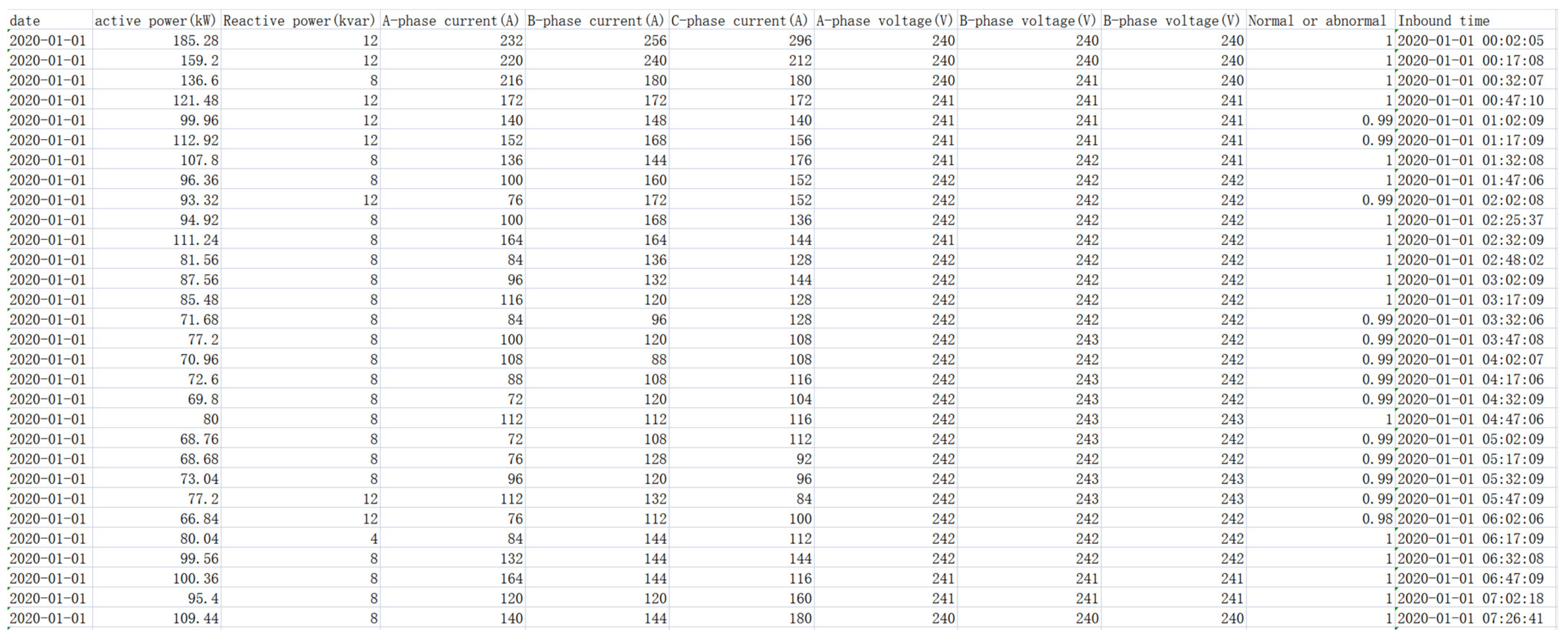
The real data were obtained from actual energy consumption data recorded in a city in the Zhejiang Province of China for one year in 2020, collected every fifteen minutes. A partial screenshot of the dataset is shown in Figure 7. To measure the effectiveness of the electricity data anomaly detection algorithm, these data were manually labeled, meaning that any anomalies have been identified. These labels were used only when evaluating the strengths and weaknesses of the algorithm and were not used in model training. The parameters of the model are reported in Table 10.

3.3.1. Real Data Prediction

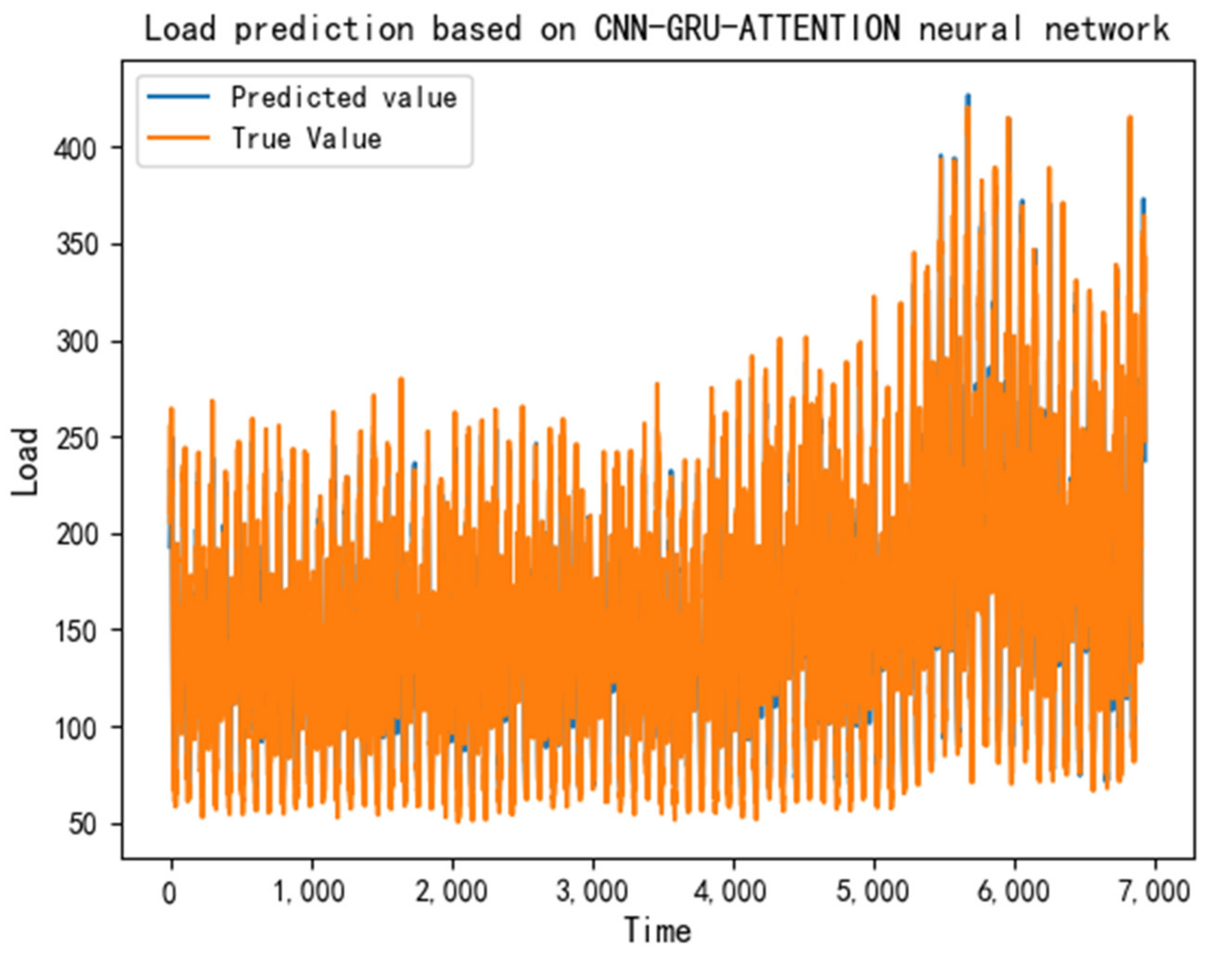
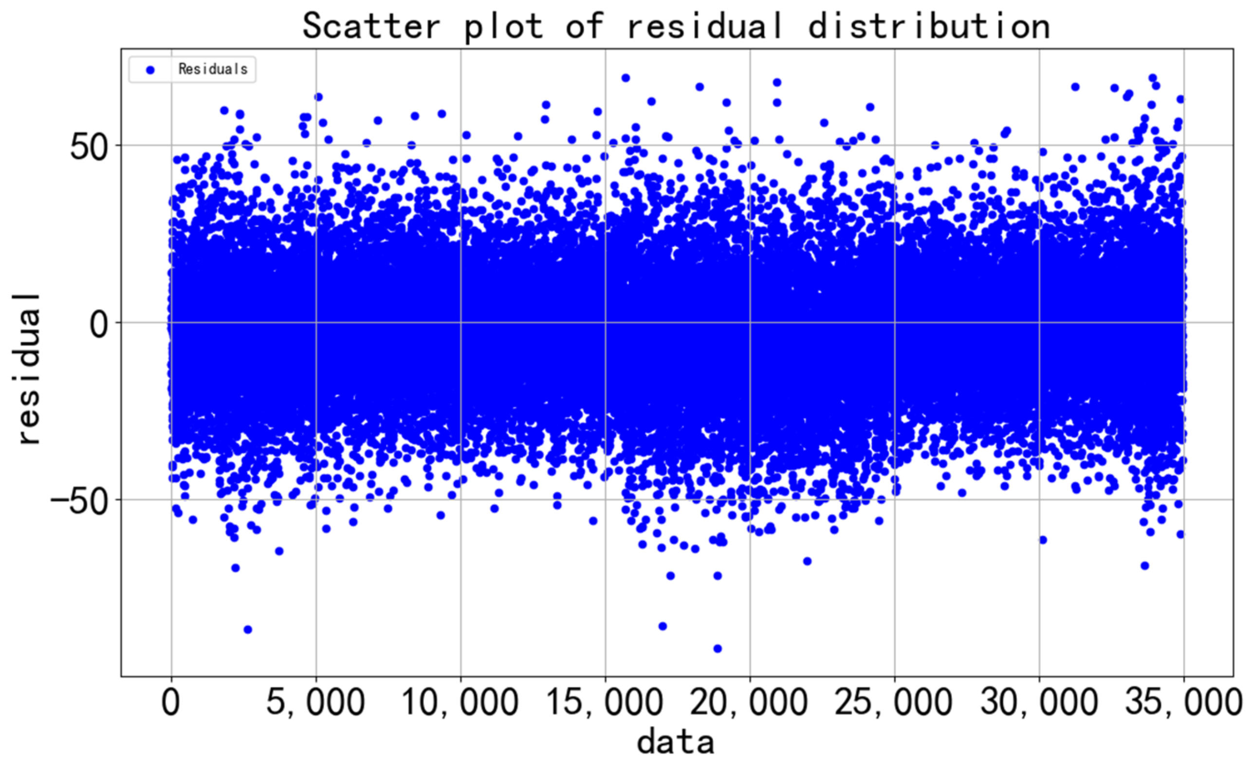
Figure 8 shows the prediction results compared to the original data. It is clear that the prediction model forecasts items very effectively for real data. The quantitative results are shown in Table 9. Imperfections in prediction results are to be expected as there are outliers in the original data, which are to be identified. The new sequence of residuals reconstructed after prediction, shown in Figure 9, is used for the next step of outlier detection.
Table 11 shows the experimental results of comparing the CNN-GRU-ATTENTION prediction model used in this study with several other classical prediction models. In terms of RMSE, the method here is 6.056, 30.089, and 4.536 lower than for CNN, GRU, and CNN-GRU, respectively; MSE is 510.064, 2191.232, and 442.583 lower; MPAE is 4.545%, 14.349%, and 2.214% lower; MAE is 5.55, 25.812, 3.361 lower; and R2 improved by 0.056, 0.162, 0.04. The method of this research has significantly improved five prediction evaluation indices compared with the other three methods, and the prediction accuracy is relatively high. Overall, it seems that the prediction method chosen for study has the best prediction performance.

3.3.2. Outlier Detection

The CGA-RF method selected for anomaly detection in this study was compared with the RandomForest classification algorithm, DecisionTree classification algorithm, and AdaBoost classification algorithm. The anomaly detection methods for comparison used normalized energy consumption data as input, while the method in this study first models the temporal characteristics of electricity consumption data using a CNN-GRU model based on a self-focus mechanism and performs prediction to obtain a prediction sequence. Then, the predicted and true values are subtracted to obtain a new sequence of residuals, which is classified using a random forest classification algorithm optimized by grid search to identify anomalies. In this study, accuracy, precision, recall, and F1 score were selected as evaluation criteria for the detection effectiveness of all methods.
Detection results are shown in Table 12. We applied DecisionTree, AdaBoost, RandomForest, and GridSearchCV-RandomForest to detect outliers in the load data. It is clear that the random forest algorithm optimized by grid search shows better overall detection advantages compared with other algorithms in this research, detecting 1624 outliers with 95.9% accuracy, 96.4% precision, 89.3% recall, and an F1 score of 0.933. Among them, the decision tree algorithm, although performing relatively well in the number of detected anomalies, detected 369 fewer anomalies than the research method in this paper. Although AdaBoost detected more anomalies, it misclassified 3813 points as normal and the detection performance was poor. The random forest algorithm without grid search parameter optimization, however, can be seen to have lower detection ability than the random forest algorithm with grid search parameter optimization in several evaluation metrics. In addition, the method in this study achieves the highest recall rate, which means that relatively more outlier points are found. On the one hand, this is due to the fact that the model uses CNN-GRU based on a self-attentive mechanism to model the temporal correlation of power data, which better utilizes historical information to predict data at the current moment and thus reconstructs the load sequence, making it easier to distinguish normal data from abnormal data in the new sequence of residuals. Finally, the results of the GridSearchCV-RandomForest algorithm and other comparative models show the advantage of GridSearchCV-RandomForest in detecting anomalies with asymmetric distribution.

4. Conclusions

In this study, a combined CNN-GRU prediction model was proposed based on a self-attentive mechanism and a random forest detection model based on grid search optimization (CGA-RF) for targeted detection of anomalies in time series energy consumption data. The central points of the full study are summarized as follows.
(1) Combining the CNN-GRU-ATTENTION model with the GridSearchCV-RandomForest model, the CNN-GRU-ATTENTION model makes full use of a CNN to extract the feature vectors of energy consumption data, and then of the GRU to accurately model its dynamic changes. The attention mechanism layer then probabilistically assigns important resources, enhances the selection of important information, and makes full use of historical information to predict power consumption at any given moment. The use of integrated learning methods such as random forest for anomaly detection of residual terms of predicted and true values can effectively improve the accuracy of detection, while the grid search parameter optimization method can reduce the manual tuning time for parameters and effectively improve the speed and efficiency of anomaly detection.
(2) Energy consumption data essentially satisfy time series distribution in terms of time series characteristics such as trend, periodicity, and seasonality. An empirical analysis of the selected combined method (CGA-RF) for anomaly detection from actual energy consumption data in this paper verifies the effectiveness of the method for anomaly detection of electricity consumption data.
(3) The current combination of the CNN-GRU model based on the self-attention mechanism and the GridSearchCV-RandomForest algorithm can only detect anomalies at a single point in time in electricity consumption data. In future studies, a method to detect and identify anomalous time periods can be considered. Meanwhile, since the method selected in this study mainly focuses on high accuracy prediction, subsequent research can be performed to further develop the accuracy of the prediction model.

Author Contributions

Conceptualization, C.L., D.L. and S.X.; Methodology, C.L., D.L. and H.W.; Investigation, M.W.; Writing—original draft, C.L. All authors have read and agreed to the published version of the manuscript.

Funding

This research received no external funding.

Data Availability Statement

The data presented in this study are available on request from the first author.

Conflicts of Interest

The authors declare no conflict of interest.

References

  1. Lan, T.; Lin, Y.; Wang, J.; Leao, B.; Fradkin, D. Unsupervised Power System Event Detection and Classification Using Unlabeled PMU Data. In Proceedings of the 2021 IEEE PES Innovative Smart Grid Technologies Europe (ISGT Europe), Espoo, Finland, 18–21 October 2021; pp. 1–5. [Google Scholar] [CrossRef]
  2. Rao, S.; Muniraju, G.; Tepedelenlioglu, C.; Srinivasan, D.; Tamizhmani, G.; Spanias, A. Dropout and Pruned Neural Networks for Fault Classification in Photovoltaic Arrays. IEEE Access 2021, 9, 120034–120042. [Google Scholar] [CrossRef]
  3. Mandhare, H.C.; Idate, S.R. A comparative study of cluster based outlier detection, distance based outlier detection and density based outlier detection techniques. In Proceedings of the 2017 International Conference on Intelligent Computing and Control Systems (ICICCS), Madurai, India, 15–16 June 2017; pp. 931–935. [Google Scholar] [CrossRef]
  4. Wang, H.; Bah, M.J.; Hammad, M. Progress in Outlier Detection Techniques: A Survey. IEEE Access 2019, 7, 107964–108000. [Google Scholar] [CrossRef]
  5. Nascimento, G.F.M.; Wurtz, F.; Kuo-Peng, P.; Delinchant, B.; Batistela, N.J. Outlier Detection in Buildings’ Power Consumption Data Using Forecast Error. Energies 2021, 14, 8325. [Google Scholar] [CrossRef]
  6. Li, T.; Comer, M.L.; Delp, E.J.; Desai, S.R.; Mathieson, J.L.; Foster, R.H.; Chan, M.W. Anomaly Scoring for Prediction-Based Anomaly Detection in Time Series. In Proceedings of the 2020 IEEE Aerospace Conference, Big Sky, MT, USA, 7–14 March 2020; pp. 1–7. [Google Scholar] [CrossRef]
  7. Salleh, N.S.M.; Saripuddin, M.; Suliman, A.; Jorgensen, B.N. Electricity Anomaly Point Detection using Unsupervised Technique Based on Electricity Load Prediction Derived from Long Short-Term Memory. In Proceedings of the 2021 2nd International Conference on Artificial Intelligence and Data Sciences (AiDAS), Ipoh, Malaysia, 8–9 September 2021; pp. 1–5. [Google Scholar] [CrossRef]
  8. Zhou, Q.; Liu, F.; Gong, H. Robust three-vector model predictive torque and stator flux control for PMSM drives with prediction error compensation. J. Power Electron. 2022, 22, 1917–1926. [Google Scholar] [CrossRef]
  9. Zhu, R.; Wang, P. Adaptive Control of Nonlinear System Under Input Constraints Combined with Prediction-Error Estimation for Uncertainty. In Proceedings of the 2022 IEEE 17th International Conference on Control & Automation (ICCA), Naples, Italy, 27–30 June 2022; pp. 63–67. [Google Scholar] [CrossRef]
  10. Madhusudhanan, A.K.; Na, X.; Ainalis, D.; Cebon, D. Engine Fuel Consumption Modelling Using Prediction Error Identification and On-Road Data. Available online: http://eprints.soton.ac.uk/id/eprint/457356 (accessed on 29 December 2022).
  11. Zhang, S.; Zhang, G.; Zhang, K. Coordinated Control Strategy of Wind-Photovoltaic Hybrid Energy Storage Considering Prediction Error Compensation and Fluctuation Suppression. In Proceedings of the 2021 IEEE 2nd International Conference on Information Technology, Big Data and Artificial Intelligence (ICIBA), Chongqing, China, 17–19 December 2021; pp. 1185–1189. [Google Scholar] [CrossRef]
  12. Peñaloza, A.K.A.; Balbinot, A.; Leborgne, R.C. “Review of Deep Learning Application for Short-Term Household Load Forecasting. In Proceedings of the 2020 IEEE PES Transmission & Distribution Conference and Exhibition—Latin America (T&D LA), Montevideo, Uruguay, 28 September–2 October 2020; pp. 1–6. [Google Scholar] [CrossRef]
  13. Shahi, T.B.; Shrestha, A.; Neupane, A.; Guo, W. Stock Price Forecasting with Deep Learning: A Comparative Study. Mathematics 2020, 8, 1441. [Google Scholar] [CrossRef]
  14. Jung, S.; Moon, J.; Park, S.; Hwang, E. An Attention-Based Multilayer GRU Model for Multistep-Ahead Short-Term Load Forecasting. Sensors 2021, 21, 1639. [Google Scholar] [CrossRef]
  15. Meng, Z.; Xie, Y.; Sun, J. Short-term load forecasting using neural attention model based on EMD. Electr. Eng. 2022, 104, 1857–1866. [Google Scholar] [CrossRef]
  16. Park, J.; Hwang, E. A Two-Stage Multistep-Ahead Electricity Load Forecasting Scheme Based on LightGBM and Attention-BiLSTM. Sensors 2021, 21, 7697. [Google Scholar] [CrossRef]
  17. Lin, T.; Pan, Y.; Xue, G.; Song, J.; Qi, C. A Novel Hybrid Spatial-Temporal Attention-LSTM Model for Heat Load Prediction. IEEE Access 2020, 8, 159182–159195. [Google Scholar] [CrossRef]
  18. Xia, X.; Togneri, R.; Sohel, F.; Huang, D. Random forest classification based acoustic event detection. In Proceedings of the 2017 IEEE International Conference on Multimedia and Expo (ICME), Munich, Germany, 16 November 2017; pp. 163–168. [Google Scholar] [CrossRef]
  19. Nagaraj, P.; Muneeswaran, V.; Deshik, G. Ensemble Machine Learning (Grid Search & Random Forest) based Enhanced Medical Expert Recommendation System for Diabetes Mellitus Prediction. In Proceedings of the 2022 3rd International Conference on Electronics and Sustainable Communication Systems (ICESC), Coimbatore, India, 17–19 August 2022; pp. 757–765. [Google Scholar] [CrossRef]
  20. Siji George, C.G.; Sumathi, B. Grid Search Tuning of Hyperparameters in Random Forest Classifier for Customer Feedback Sentiment Prediction. Int. J. Adv. Comput. Sci. Appl. IJACSA 2020, 11, 173–178. [Google Scholar]
  21. Abokhzam, A.A.; Gupta, N.K.; Bose, D.K. Efficient diabetes mellitus prediction with grid based random forest classifier in association with natural language processing. Int. J. Speech Technol. 2021, 24, 601–614. [Google Scholar] [CrossRef]
  22. Shi, H.; Wang, L.; Scherer, R.; Wozniak, M.; Zhang, P.; Wei, W. Short-Term Load Forecasting Based on Adabelief Optimized Temporal Convolutional Network and Gated Recurrent Unit Hybrid Neural Network. IEEE Access 2021, 9, 66965–66981. [Google Scholar] [CrossRef]
  23. Pavićević, M.; Popović, T. Forecasting Day-Ahead Electricity Metrics with Artificial Neural Networks. Sensors 2022, 22, 1051. [Google Scholar] [CrossRef]
  24. Ayub, N.; Irfan, M.; Awais, M.; Ali, U.; Ali, T.; Hamdi, M.; Alghamdi, A.; Muhammad, F. Big Data Analytics for Short and Medium-Term Electricity Load Forecasting Using an AI Techniques Ensembler. Energies 2020, 13, 5193. [Google Scholar] [CrossRef]
  25. Liu, K.; Hu, X.; Zhou, H.; Tong, L.; Widanalage, D.; Marco, J. Feature Analyses and Modelling of Lithium-ion Batteries Manufacturing based on Random Forest Classification. IEEE/ASME Trans. Mechatron. 2021, 26, 2944–2955. [Google Scholar] [CrossRef]
  26. Sales, M.H.R.; de Bruin, S.; Souza, C.; Herold, M. Land Use and Land Cover Area Estimates from Class Membership Probability of a Random Forest Classification. IEEE Trans. Geosci. Remote. Sens. 2022, 60, 4402711. [Google Scholar] [CrossRef]
  27. Zhang, L.; Liu, K.; Wang, Y.; Omariba, Z.B. Ice Detection Model of Wind Turbine Blades Based on Random Forest Classifier. Energies 2018, 11, 2548. [Google Scholar] [CrossRef] [Green Version]
  28. Xiong, F.; Cao, C.; Tang, M.; Wang, Z.; Tang, J.; Yi, J. Fault Detection of UHV Converter Valve Based on Optimized Cost-Sensitive Extreme Random Forest. Energies 2022, 15, 8059. [Google Scholar] [CrossRef]
  29. Sun, Y.; Que, H.; Cai, Q.; Zhao, J.; Li, J.; Kong, Z.; Wang, S. Borderline SMOTE Algorithm and Feature Selection-Based Network Anomalies Detection Strategy. Energies 2022, 15, 4751. [Google Scholar] [CrossRef]
  30. Dudek, G. A Comprehensive Study of Random Forest for Short-Term Load Forecasting. Energies 2022, 15, 7547. [Google Scholar] [CrossRef]
  31. Lu, Y.; Li, Y.; Xie, D.; Wei, E.; Bao, X.; Chen, H.; Zhong, X. The Application of Improved Random Forest Algorithm on the Prediction of Electric Vehicle Charging Load. Energies 2018, 11, 3207. [Google Scholar] [CrossRef] [Green Version]
  32. Chi, Y.; Zhang, Y.; Li, G.; Yuan, Y. Prediction Method of Beijing Electric-Energy Substitution Potential Based on a Grid-Search Support Vector Machine. Energies 2022, 15, 3897. [Google Scholar] [CrossRef]
  33. Xia, D.; Zheng, Y.; Bai, Y.; Yan, X.; Hu, Y.; Li, Y.; Li, H. A parallel grid-search-based SVM optimization algorithm on Spark for passenger hotspot prediction. Multimedia Tools Appl. 2022, 81, 27523–27549. [Google Scholar] [CrossRef]
  34. Zhang, J.; Wang, J.; Wei, M.; Zheng, Y.; Yang, Z. Optimal PI controller tuning for dynamic TITO systems with rate-limiters based on parallel grid search. In Proceedings of the 2021 33rd Chinese Control and Decision Conference (CCDC), Kunming, China, 22–24 May 2021; pp. 5808–5811. [Google Scholar] [CrossRef]
  35. Kaewwiset, T.; Temdee, P. Promotion Classification Using DecisionTree and Principal Component Analysis. In Proceedings of the 2022 Joint International Conference on Digital Arts, Media and Technology with ECTI Northern Section Conference on Electrical, Electronics, Computer and Telecommunications Engineering (ECTI DAMT & NCON), Chiang Rai, Thailand, 26–28 January 2022; pp. 489–492. [Google Scholar] [CrossRef]
  36. Sadouni, O.; Zitouni, A. Task-based Learning Analytics Indicators Selection Using Naive Bayes Classifier and Regression Decision Trees. In Proceedings of the 2021 International Conference on Theoretical and Applicative Aspects of Computer Science (ICTAACS), Skikda, Algeria, 15–16 December 2021; pp. 1–8. [Google Scholar] [CrossRef]
  37. Rahman, A.; Akter, Y.A. Topic Classification from Text Using Decision Tree, K-NN and Multinomial Naïve Bayes. In Proceedings of the 2019 1st International Conference on Advances in Science, Engineering and Robotics Technology (ICASERT), Dhaka, Bangladesh, 3–5 May 2019; pp. 1–4. [Google Scholar] [CrossRef]
  38. Zheng, H.; Xiao, F.; Sun, S.; Qin, Y. Brillouin Frequency Shift Extraction Based on AdaBoost Algorithm. Sensors 2022, 22, 3354. [Google Scholar] [CrossRef]
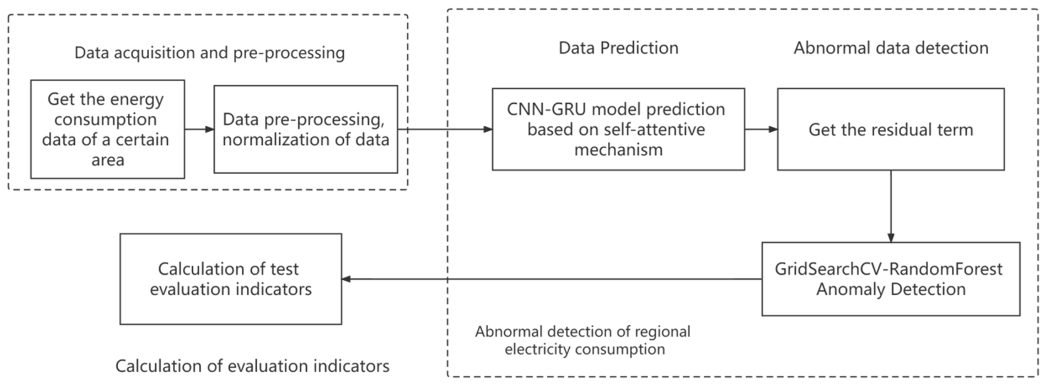
Figure 1. CGA-RF abnormal data detection flow chart.
Energies 16 00582 g001
Figure 2. Structure of CNN-GRU model based on attention mechanism.
Energies 16 00582 g002
Figure 3. Random forest classification model.
Energies 16 00582 g003
Figure 4. Hyper-parameter tuning architecture.
Energies 16 00582 g004
Figure 5. Load prediction based on CNN-GRU-ATTENTION neural network.
Energies 16 00582 g005
Figure 6. Load prediction based on CNN-GRU-ATTENTION neural network.
Energies 16 00582 g006
Figure 7. Partial screenshots of real data sets.
Energies 16 00582 g007
Figure 8. Real data predicted value vs. real value.
Energies 16 00582 g008
Figure 9. Residual distribution chart.
Energies 16 00582 g009
Table 1. Spanish Wind Power Dataset Model Parameters.
Parameters of the ModelValue
CNN layer1
Pooling layer1
Activation functionReLU
Dropout0.1
GRU layer2
Learning Rate0.01
ATTENTION20
Dense1
Activation functionReLU
Epoch30
Table 2. Comparison of forecast accuracy by month.
DateModelEvaluation Indicators
RMSEMSEMAPEMAER2
7.7–7.13CNN1135.9411,290,361.63212.214585.2380.778
GRU1255.1481,575,397.08619.12806.5720.729
CNN-GRU1021.1711,042,789.91312.725550.9380.821
CNN-GRU-ATTENTION954.175910,450.6568.769421.4740.843
8.9–8.15CNN850.32723,044.91519.473670.680.861
GRU1046.2841,094,710.07825.731827.5410.789
CNN-GRU528.219279,015.32212.111385.3550.946
CNN-GRU-ATTENTION381.397145,463.4166.923225.5260.972
9.3–9.10CNN899.017808,231.02518.751582.620.81
GRU910.147828,368.46618.7579.0170.806
CNN-GRU813.783662,242.69817.11462.6290.845
CNN-GRU-ATTENTION715.628512,124.11411.532343.9450.88
10.10–10.6CNN1136.6441,291,958.96521.276953.5560.814
GRU1367.0211868745.2727.6031211.3530.731
CNN-GRU733.993538,745.20615.761590.7260.922
CNN-GRU-ATTENTION271.68373,811.5184.718210.270.989
11.11–11.17CNN552.078304,790.53517.406381.7620.83
GRU723.403523,311.33726.181586.9180.708
CNN-GRU568.095322,731.95317.555391.8090.82
CNN-GRU-ATTENTION444.987198,013.86112.606261.4760.89
12.20–12.26CNN704.854496,819.76615.71565.2750.896
GRU939.185882,067.5519.323825.0930.816
CNN-GRU545.412297,474.43613.008447.4830.938
CNN-GRU-ATTENTION299.29589,577.4876.884239.8140.981
Table 3. Australian Load Output Dataset Model Parameters.
Parameters of the ModelValue
CNN layer1
Pooling layer1
Activation functionReLU
Dropout0.2
GRU layer2
Learning Rate0.01
ATTENTION50
Dense1
Activation functionReLU
Epoch30
Table 4. Comparison of prediction accuracy for consecutive weeks.
DateModelEvaluation Indicators
RMSEMSEMAPEMAER2
11.5CNN242.51358,812.3143.032197.9260.868
GRU249.60362,301.7583.12204.3260.861
CNN-GRU161.2826,011.3571.987128.5450.942
CNN-GRU-ATTENTION87.4727651.3731.04869.2020.983
11.6CNN224.03850,192.9632.661171.8890.9
GRU238.85157,049.8042.924192.6010.887
CNN-GRU191.5536,691.2222.194142.6460.927
CNN-GRU-ATTENTION87.5847670.9731.07271.0590.985
11.7CNN204.2641,722.3522.371161.4880.912
GRU217.89447,477.8972.547174.9750.899
CNN-GRU163.28726,662.5511.946133.390.944
CNN-GRU-ATTENTION135.81418,445.3671.761118.0730.961
11.8CNN226.87451,472.0172.718194.5020.913
GRU184.29933,966.0422.098147.5270.943
CNN-GRU154.42923,848.3641.668115.8110.96
CNN-GRU-ATTENTION114.10313,019.5671.39896.3970.978
11.9CNN252.163,554.3072.836196.7090.902
GRU254.58264,811.783.18224.1290.9
CNN-GRU191.68236,741.8172.092145.0750.943
CNN-GRU-ATTENTION144.51220,883.6041.528108.1240.968
11.10.CNN307.48694,547.4923.843260.0320.871
GRU220.71848,716.2692.607181.4170.934
CNN-GRU200.24340,097.3872.239152.1550.945
CNN-GRU-ATTENTION11012,099.9791.24686.3420.983
11.11CNN274.76875,497.4053.285227.8670.9
GRU383.623147,166.8454.283300.4850.804
CNN-GRU311.18796,837.0653.637251.120.871
CNN-GRU-ATTENTION127.85916,348.0291.37796.9110.978
Table 5. FreezerRegularTrain dataset.
True
Positives
False
Negatives
False
Positives
AccuracyPrecisionRecallF1 Score
DecisionTree12611641570.8870.8890.8840.887
AdaBoost137055990.9470.9320.9610.946
RandomForest1402231170.8410.9520.9500.950
GridSearchCV-RandomForest1402231200.9490.9510.9490.949
Table 6. PowerCons dataset.
True
Positives
False
Negatives
False
Positives
AccuracyPrecisionRecallF1 Score
DecisionTree90020.9880.9781.00.989
AdaBoost90001.01.01.01.0
RandomForest90001.01.01.01.0
GridSearchCV-RandomForest90001.01.01.01.0
Table 7. Wafer dataset.
True
Positives
False
Negatives
False
Positives
AccuracyPrecisionRecallF1 Score
DecisionTree3972681210.9360.7660.5960.671
AdaBoost60560600.9800.9090.9090.909
RandomForest50316280.9720.9840.7560.855
GridSearchCV-RandomForest62045120.9920.9810.9320.956
Table 8. Italy power demand dataset.
True
Positives
False
Negatives
False
Positives
AccuracyPrecisionRecallF1 Score
DecisionTree48924150.9620.9700.9530.961
AdaBoost46548180.9350.9620.9060.933
RandomForest49716160.9680.9680.9680.968
GridSearchCV-RandomForest49815150.9340.9700.9700.970
Table 9. Mote strain dataset.
True
Positives
False
Negatives
False
Positives
AccuracyPrecisionRecallF1 Score
DecisionTree5521231440.7860.7930.8170.805
AdaBoost5701051470.7980.7940.8440.818
RandomForest60372710.8350.8940.8930.893
GridSearchCV-RandomForest61263880.8790.8740.9060.890
Table 10. Real Dataset Model Parameters.
Parameters of the ModelValue
CNN layer1
Pooling layer1
Activation functionReLU
Dropout0.2
GRU layer2
Learning Rate0.01
ATTENTION20
Dense1
Activation functionReLU
Epoch30
Table 11. Real dataset prediction results.
RMSEMSEMAPEMAER2
CNN22.959527.09413.09018.3540.879
GRU46.9922208.26222.89438.6160.773
CNN-GRU21.439459.61310.75916.1650.895
CNN-GRU-ATTENTION16.90317.030 8.54512.804 0.935
Table 12. Real dataset detection results.
True
Positives
False
Negatives
False
Positives
AccuracyPrecisionRecallF1 Score
DecisionTree12545620 0.9000.9360.8450.874
AdaBoost18011538130.3240.5130.5000.251
RandomForest1254562250.8960.9260.8420.869
GridSearchCV-RandomForest1623 193390.9590.9640.8930.933
Disclaimer/Publisher’s Note: The statements, opinions and data contained in all publications are solely those of the individual author(s) and contributor(s) and not of MDPI and/or the editor(s). MDPI and/or the editor(s) disclaim responsibility for any injury to people or property resulting from any ideas, methods, instructions or products referred to in the content.