Parallel Multi-Layer Monte Carlo Optimization Algorithm for Doubly Fed Induction Generator Controller Parameters Optimization

Abstract

This work proposes a parallel multi-layer Monte Carlo optimization algorithm (PMMCOA) that optimizes proportional–integral parameters for a doubly fed induction generator-based wind turbine controller. The PMMCOA, an improved form of the Monte Carlo algorithm, realizes the optimization process via a parallel multi-layer structure. The PMMCOA includes rough search layers, precise search layers, and re-precise search layers. Each layer of the PMMCOA adopts a multi-region and multi-granularity approach to increase the diversity and randomness of the search samples. The PMMCOA is employed to tune the controller parameters for achieving maximum power point tracking and improving generation efficiency. The controller fitness function reflects the sum of the rotor angular velocity error and the reactive power error. Compared with the five metaheuristic algorithms, the PMMCOA has a higher global convergence and more accurate power tracking ability.

1. Introduction

Nowadays, the world problem of environmental pollution and energy shortage has aroused the great attention of human society [1]. With the increasing familiarity with renewable energy, human beings have begun to utilize renewable energy such as wind, solar, biomass, tidal, hydropower, geothermal, and other renewable energy for power generation; renewable energy has dramatically alleviated the rapid shortage of conventional energy [2]. The earth is rich in wind energy, which has a high utilization value in renewable energy; therefore, wind energy development has attracted much attention [3]. Wind power is applied to generate electricity, attracting more and more scholars and researchers. With the application of aerodynamics, aerospace technology, and high-power electronic technology in new wind turbines, wind power technology has made rapid progress in the past decade [4]. 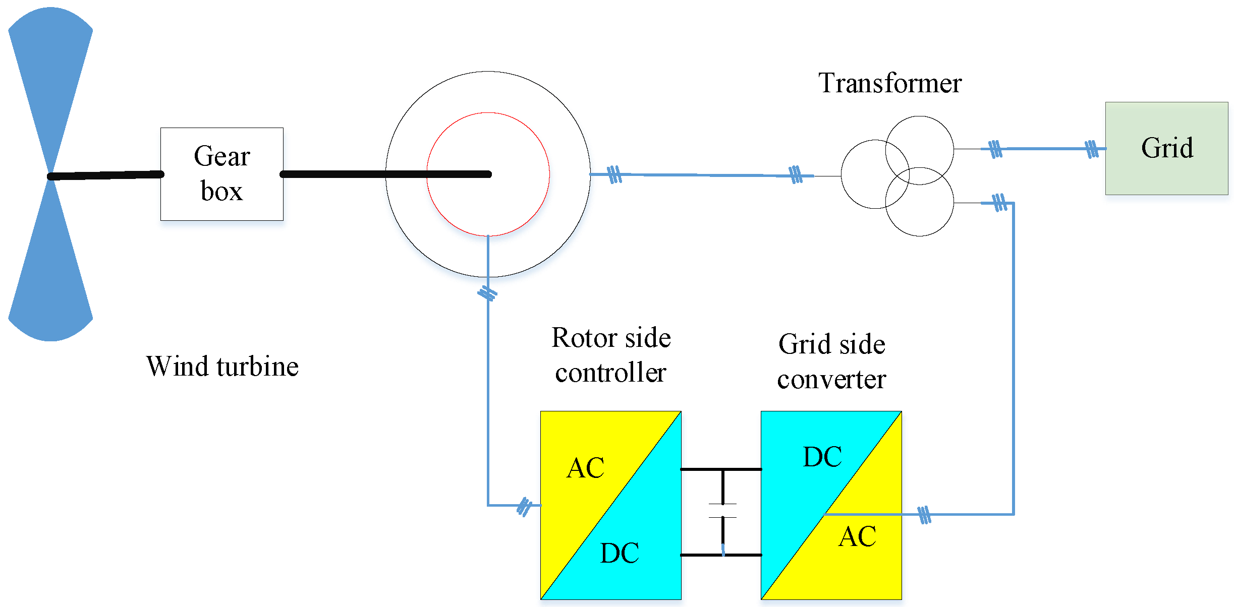In addition, with the strengthening awareness of environmental protection and the energy crisis, to promote the continuous extensionally utilization of renewable energy, countries have issued plans, which have made the enlargement momentum of the wind power industry more intense [5]. In recent years, the appearance of doubly fed induction generators (DFIGs) offering the rated capacity of wind turbines gradually increased [6]. The DFIGs can flexibly adjust the active and reactive power, operate with variable speed, track the maximum wind energy, and reduce the mechanical stress. Furthermore, the converter of the DFIGs only needs to transmit 25–30% slip power of the rated power. Therefore, the converter of the DFIGs has the characteristics of small capacity and low cost [7]. Thus, the DFIGs have been widely applied in high-power wind power generation [8]. The particle swarm optimization (PSO) algorithm-based optimized controller improves the dynamic performance of DFIG-based wind power systems [9]. The proportional–integral (PI) parameters of the converter in the grid-connected DFIG are optimized via a genetic algorithm (GA). The optimized converter can improve the working reliability of the unit, prolong the use time of the unit, and expand the stable operation area of the wind farm [10]. 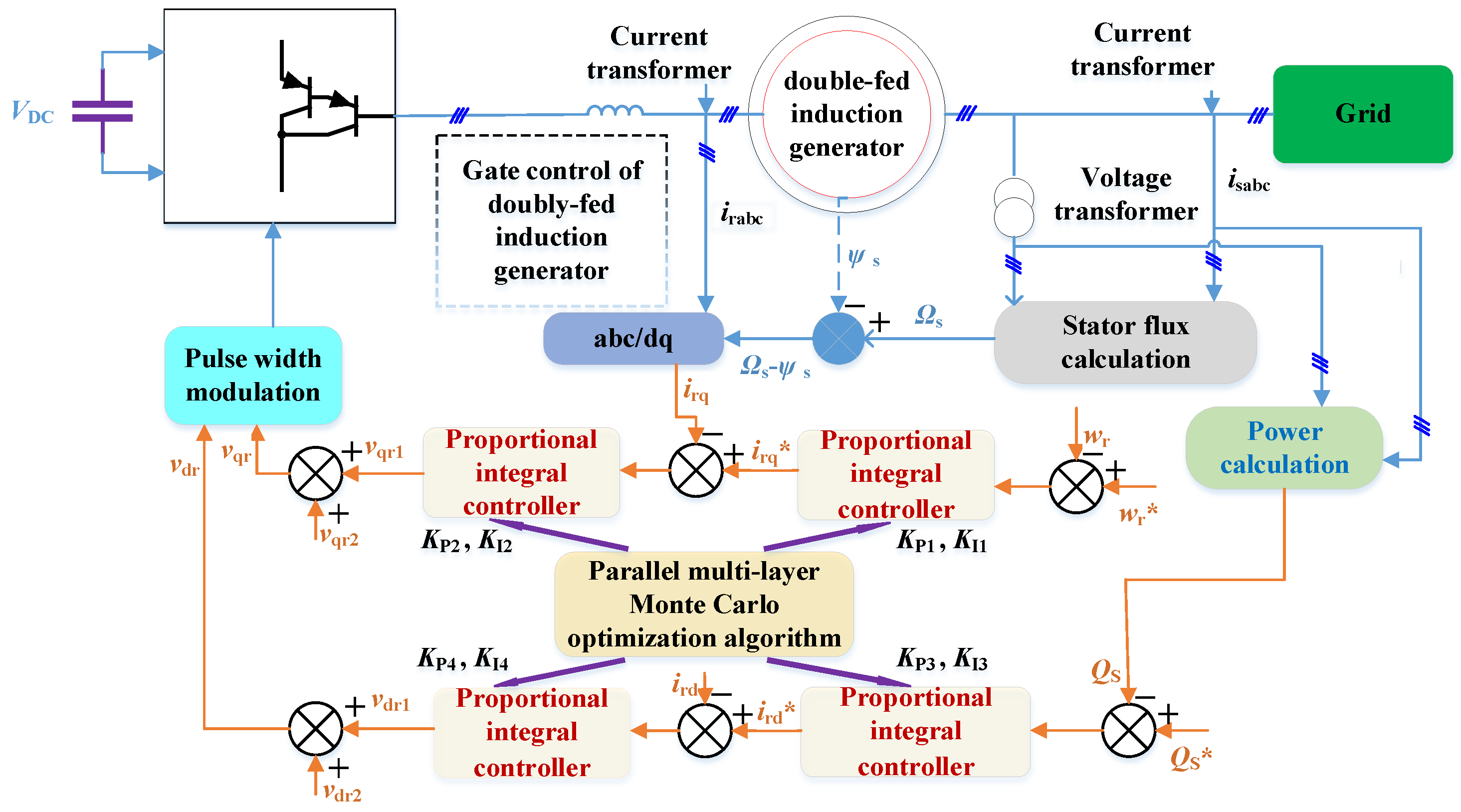A chemical reaction optimization algorithm is used to tune the optimal PI parameters, which then ensures optimal power point tracking of the DFIG-based wind power system [11]. In the DFIGs-based wind power system, the PI parameters of the rotor-side controller (RSC) can be optimized to make the rotor angular velocity track the optimal rotational speed at the wind speed as much as possible according to the random mutation of the wind speed, which can help to increase the wind power conversion rate of the system, and at the same time, improve the control performance of the RSC as much as possible. Generally, the control parameters of the DFIGs can be manually adjusted based on the linearized model of the original DFIGs for a particular operating condition; however, the control performance may be significantly degraded with the continuous change in the operating conditions. Therefore, to adapt to the different operating conditions, it is indispensable to find a reliable and effective method to adjust the optimal PI control parameters based on various operating conditions.

Wind turbines are generally related to the actual wind conditions and require maximum wind energy utilization [12]. Therefore, the study on letting the wind turbines output the maximum power under different wind speeds is of practical significance and economic benefit. Maximum power point tracking (MPPT) has been one of the major control targets for picking up the maximum power of wind turbines to the greatest extent [13]. Numerous studies have focused on realizing the MPPT for the DFIGs and proposed some implementation methods [14]. The real-time MPPT algorithm has the advantage that maximum power tracking can be achieved by adjusting the reference power curve when the system parameters change slightly [15]. Tip-speed ratio control maintenance at the optimal point has been applied in the MPPT of a DFIG [16]. R. Garduno and M. Borunda et al. proposed a fuzzy controller to extract wind power [17]. K. Tahir and C. Belfedal et al. adjusted and dominated the torque of the wind turbine from the perspective of torque control to achieve the MPPT [18]. The hill-climbing searching algorithm can adjust the rotor velocity of the DFIG under different operating conditions and enhance the energy conversion efficiency [19,20]. The improved variable step hill-climbing searching algorithm has been proposed to implement MPPT for wind turbines [21].

In the methods mentioned above, the optimal control signal can be calculated using the estimated wind speeds. Nevertheless, the control strategies of these methods are comparatively complex. The vector combined with the PI control with a simple structure has been applied for reactive and active power decoupling control [22]. The PI controller is characterized by its reliable operation and simple structure. Furthermore, the PI control systems can be easily realized with general electronic circuits and motor equipment. Thus, the PI control occupies many industrial production control processes and is the primary control method in engineering practice [23]. Conventional optimization methods based on the gradient may not obtain the optimal parameters with the accuracy and precision of system models [24]. Numerous metaheuristic optimization algorithms have become increasingly prevalent to obtain optimal control parameters over the past two decades [25]. The metaheuristic algorithms are simple. The error index of indirect power control shows that the PI parameters tuned via the PSO algorithm are more satisfied than those manually adjusted [26]. In Ref. [27], an active power optimization dispatching strategy based on a genetic algorithm GA has been proposed in a DFIG-based wind farm. The moth flame optimization (MFO) algorithm [28] has been utilized for acquiring satisfactory parameters in the robust correlative control system in a DFIG-based wind turbine [29]. Grey wolf optimization (GWO) was proposed for optimization by Mirjalili of Griffith University in Australia in 2014. A grouped grey wolf optimizer (GGWO) has been developed to achieve maximum power extraction. A method for tuning the PI parameters has not considered the change in the control response caused by a sudden change in grid voltage [30].

The Monte Carlo method plays a vital role in numerical calculations guided by the probability and statistics theory, which can achieve approximate solutions using many random experiments, can solve definite mathematical and stochastic problems, is a powerful tool for systems analysis and design, and has been widely applied in natural science, engineering technology, and the national economy [31]. Shi et al. proposed a nested partition optimization method with global search, local search, easy implementation, parallelism, and globality [32]. In Ref. [33], a pure adaptive Monte Carlo optimization with the improvement of pure random search algorithms has been proposed. The pure adaptive search has certain flaws because an effective method that can generate a uniform distribution of random numbers within a common convex domain has not yet been found. 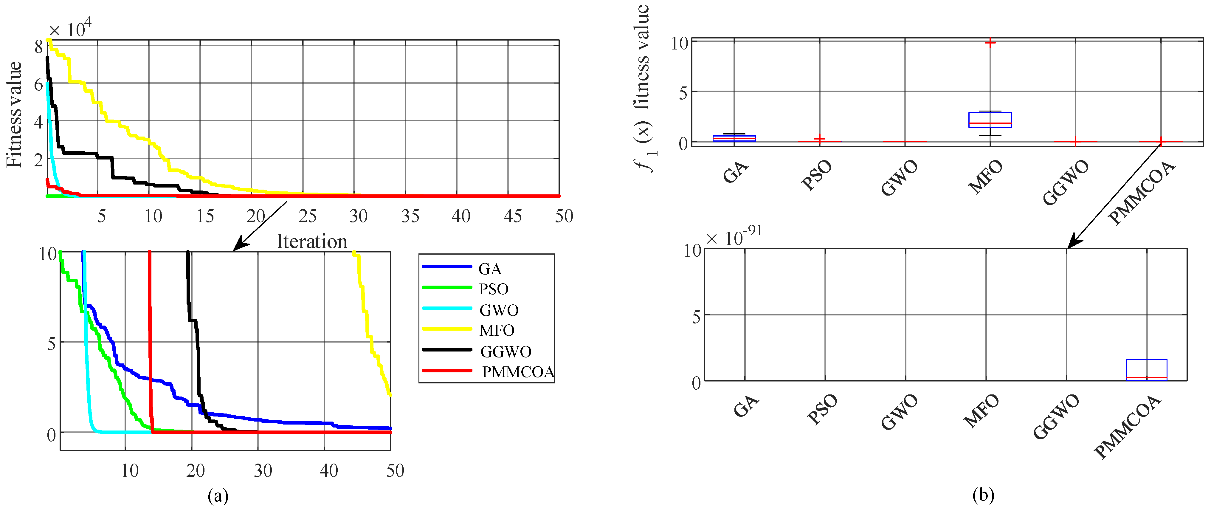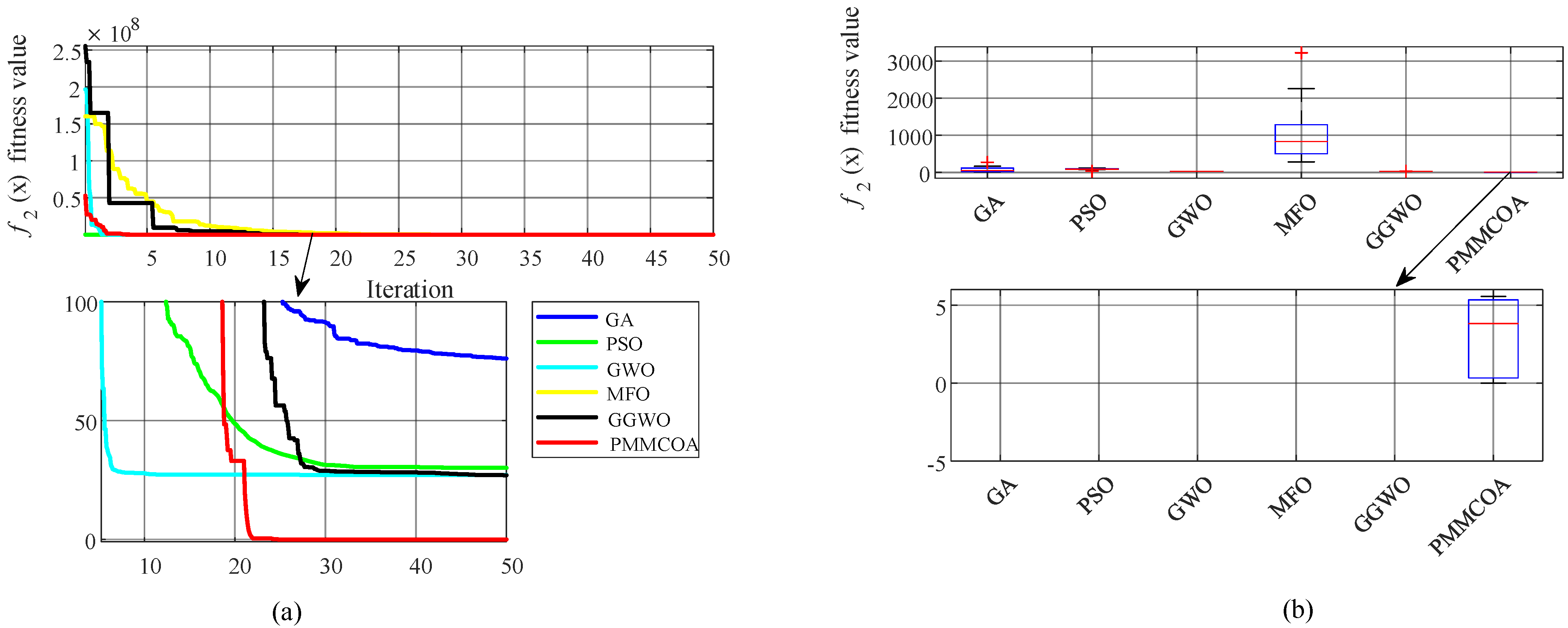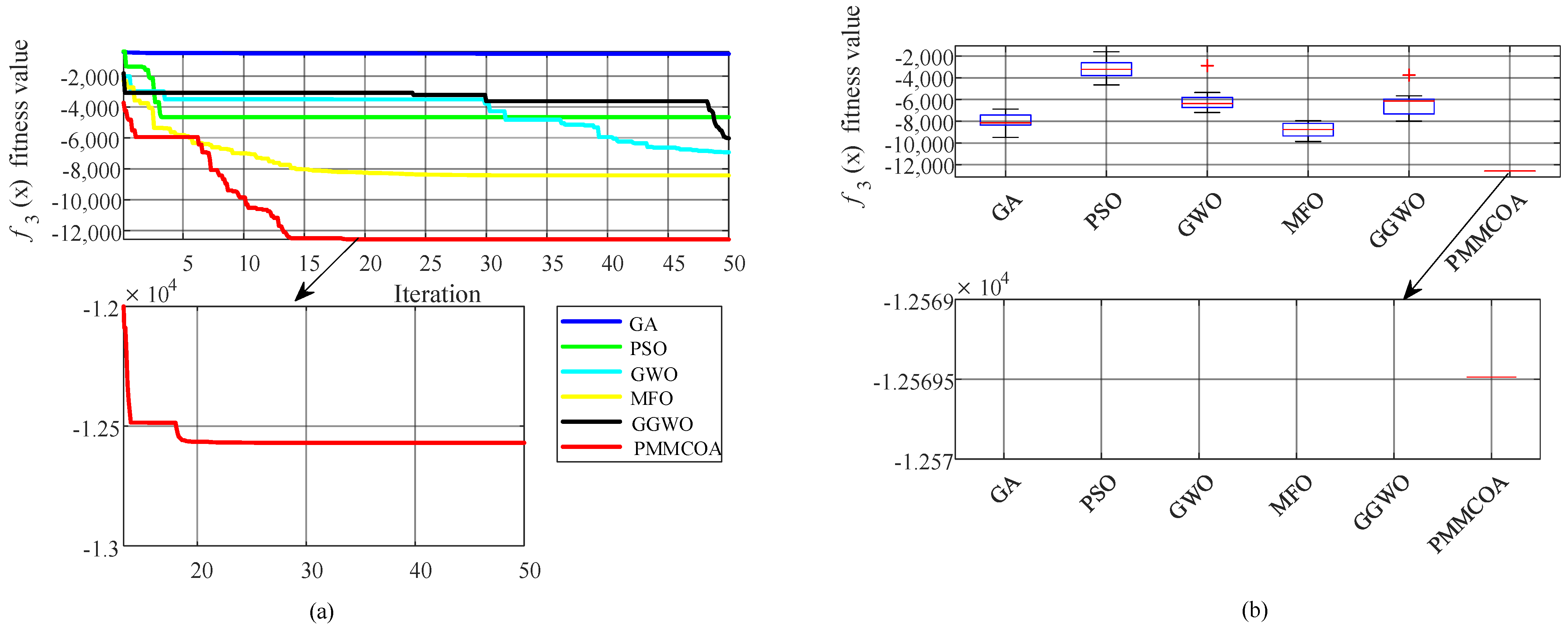The no-free lunch theorem [34] logically proves that a specific metaheuristic algorithm may find effective and reliable results on some specific issues; however, when the same algorithm is applied to other problems, bad and unrealistic results may occur [35]. The GA, the PSO, the MFO, the GWO, and the GGWO have all been employed for the parameters optimization of the DFIG-based wind turbines; however, these algorithms are underdeveloped and under-explored, which may lead to premature convergence and may not readily lead to the globally optimal parameters for DFIG-based wind turbines. The conventional Monte Carlo algorithm can theoretically obtain the global optimal PI parameters via countless experiments; however, abundant experiment time is required; consequently, the Monte Carlo method can be improved to obtain satisfactory PI parameters. To optimize the PI parameters of the rotor RSC of a DFIG-based wind power generation system, a parallel multi-layer Monte Carlo optimization algorithm (PMMCOA) is proposed for obtaining satisfactory PI parameters within DFIG-based wind turbines in this work. Two examples are tested; one applies three typical benchmark functions for proving the feasibility of the PMMCOA, and the other employs the PMMCOA to minimize the controller fitness value of a DFIG. The optimization results of the PMMCOA are compared with five representative metaheuristic algorithms. Two examples demonstrate the effectiveness and feasibility of PMMCOA in optimizing the DFIG controller parameters; meanwhile, the second example verifies that the optimized controller parameters can enable a DFIG-based wind turbine to achieve the MPPT.

This work includes the following contributions.

(1)

In this work, a new algorithm called PMMCOA is proposed. The proposed PMMCOA mainly realizes the optimization process via multiple layers, multiple regions, and multiple granularities. Compared to multiple heuristics, the PMMCOA directly employs a multi-layer randomized search, which is simple to implement and avoids lengthy parameter adjustments. The major feature of the PMMCOA is that the global search performance is strong, and the local development capability is satisfactory. Three benchmark functions verify the effectiveness and feasibility of the PMMCOA.

(2)

The PMMCOA is applied to find the parameters of the optimal PI controller.

(3)

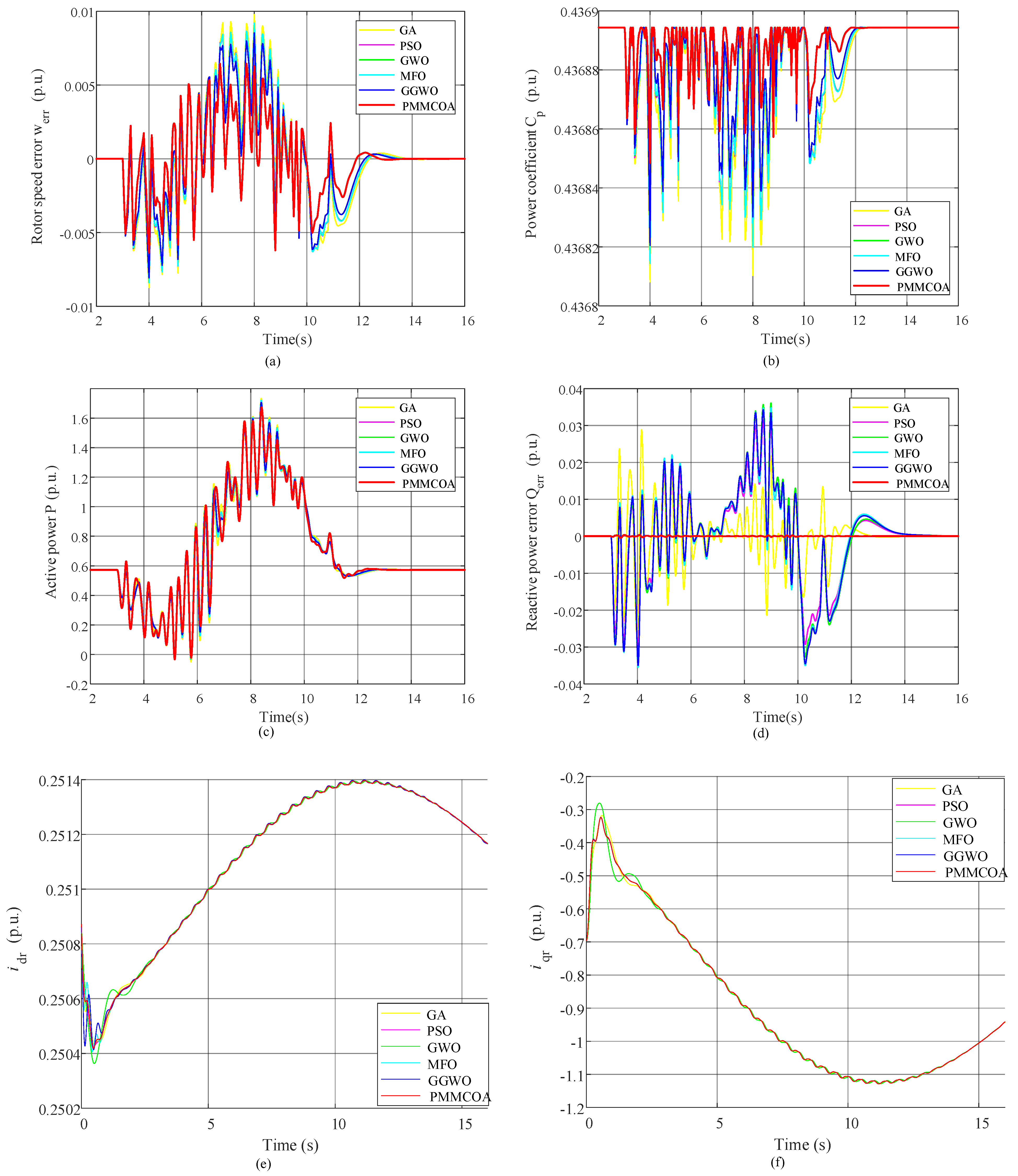
The PMMCOA-optimized controllers offer less overslip, lower volatility, and desirable efficiency for wind energy conversion. The PMMCOA grants the wind power system based on the optimized controller, which has high operating stability.

(4)

The PMMCOA-optimized controller enables the DFIG-based wind power system to implement MPPT with some ability to alleviate unexpected grid voltage variations.

(5)

Compared to other iterative processes that require references to animal behavior or brainstorming to generate optimization, the Monte Carlo stochastic approach proposed in this work is simpler and requires no optimization of many parameters.

(6)

Compared to the original heuristic algorithm that only searches at a large global scale, the layer-by-layer, spatially contracted Monte Carlo approach proposed in this work can quickly contract the feasible domains to be searched and can quickly locate the space of optimal solutions.

The remaining work is divided into four contents. The roots and procedures for implementing PMMCOA are described in Section 2. The optimal structure of the controller system based on PMMCOA for DFIG is given in Section 3. Section 4 verifies the superiority of the PMMCOA for optimizing the controller parameters. Section 5 briefly concludes this work.

2. Proposed Parallel Optimization

To achieve MPPT, a PMMCOA is proposed for acquiring satisfactory PI parameters of the RSC of DFIG-based wind turbines. Then, the PMMCOA is introduced in detail.

The Monte Carlo method can be regarded as a numerical calculation way based on “random numbers”. The vital idea of the Monte Carlo is an infinite number of sample points in the definition domain. However, the Monte Carlo calculation needs enough calculation time, and the capacity of the computer is limited. Thus, the Monte Carlo method may not be practical.

Inspired by the Monte Carlo method, this work presents a PMMCOA, which can greatly reduce the calculation time of the Monte Carlo method and obtain the minimum numerical solution approximately.

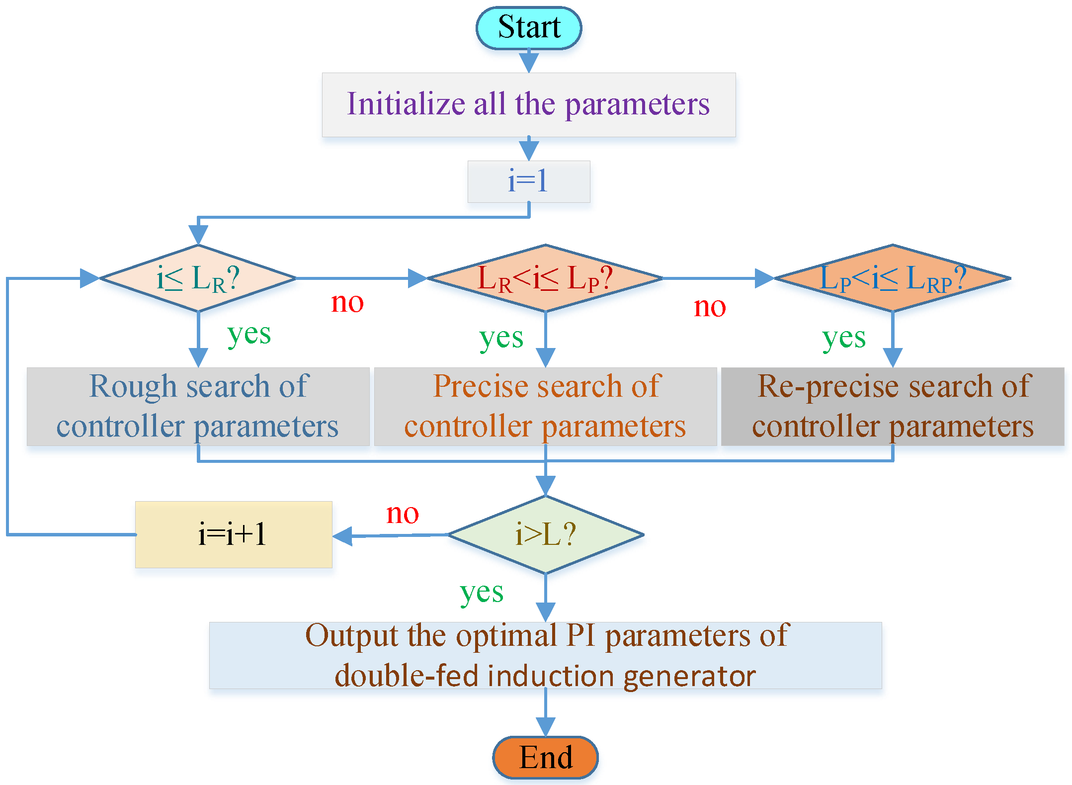
The rough, precise, and re-precise search of PMMCOA is shown in Figure 1. To facilitate the explanation, a continuous optimization problem is considered. The objective function value $f$ is calculated as

$$\left\{\begin{array}{l}minf(x)=f\left(x_1,x_2,\cdots ,x_n\right)\\ a_k⩽x_k⩽b_k;k=1,2,\cdots ,n\end{array}\right.$$

(1)

where $\left[a_k,b_k\right]$ is the domain of the variable $x_k$, and $n$ represents the spatial dimension.

2.1. Rough Search

The rough search is explained in detail. In Figure 1, the “area A” indicates the possible areas which are defined by the limit $x_k$ as $L_{\mathrm{B}k}=a_k$, $U_{\mathrm{B}k}=b_k$.

Step 1: select $m$ Monte Carlo random points at random in “area A”. ($\overrightarrow{X_{\mathrm{A}}^L}=(x_{\mathrm{A}1}^k,x_{\mathrm{A}2}^k,\cdots ,x_{\mathrm{A}m}^k)=x_{\mathrm{A}j}^k$); where $L$ denotes the current layer of the proposed algorithm, $L\in [1,M_1]$).

Step 2: the adaptation value of $\overrightarrow{X_{\mathrm{A}}^L}$ is obtained by combining $\overrightarrow{X_{\mathrm{A}}^L}$ and $f$ in Figure 1.

Step 3: different plausible domains are gained ($\{(a_{uk},b_{uk})|u\subseteq (\mathrm{B},\mathrm{C},\mathrm{D})\}$ by redefining the top and bottom borders around $\overrightarrow{X_{\mathrm{A}.\min 123}^L}$, where the $(a_{uk},b_{uk})$ is shown in Equation (2); $c1=2$; $\overrightarrow{X_{\mathrm{replace}}^L}=\overrightarrow{X_{\mathrm{A}.\min 123}^L}$), as shown in “areas B, C, and D”.

$$\left\{\begin{array}{l}{a}_{uk}=\max \{\overrightarrow{X_{\mathrm{replace}}^L}-(\frac{(U_{\mathrm{B}k}-L_{\mathrm{B}k})}{c1}-\frac{((U_{\mathrm{B}k}-L_{\mathrm{B}k})}{c1})\cdot \frac{L}{M_1}),L_{\mathrm{B}k}\}\\ b_{uk}=\min \{\overrightarrow{X_{\mathrm{replace}}^L}+(\frac{(U_{\mathrm{B}k}-L_{\mathrm{B}k})}{c1}-\frac{((U_{\mathrm{B}k}-L_{\mathrm{B}k})}{c1})\cdot \frac{L}{M_1}),U_{\mathrm{B}k}\}\end{array}\right.$$

(2)

Step 4: select $m$ Monte Carlo random points at random in “area C” ($\overrightarrow{X_{\mathrm{C}}^L}=x_{\mathrm{C}j}^k$). The adaptation value of $\overrightarrow{X_{\mathrm{C}}^L}$ is obtained by combining $\overrightarrow{X_{\mathrm{C}}^L}$ and $f$.

Step 5: $\overrightarrow{X_{\mathrm{C}.\min 12}^L}$ ($\{(a_{uk},b_{uk})|u\subseteq (\mathrm{E},\mathrm{F})\}$, where the $(a_{uk},b_{uk})$ is shown in Equation (2); $c1=4$; $\overrightarrow{X_{\mathrm{replace}}^L}=\overrightarrow{X_{\mathrm{C}.\min 12}^L}$).

Step 6: select $m$ Monte Carlo random points at random in “area D” ($\overrightarrow{X_{\mathrm{D}}^L}=x_{\mathrm{D}j}^k$).

Step 7: “area G” is obtained ($\{(a_{uk},b_{uk})|u\subseteq (\mathrm{G})\}$ by defining the top and bottom bounds around $\overrightarrow{X_{\mathrm{D}.\min 1}^L}$, where the $(a_{uk},b_{uk})$ is shown in Equation (2); $c1=6$; $\overrightarrow{X_{\mathrm{replace}}^L}=\overrightarrow{X_{\mathrm{D}.\min 1}^L}$).

Step 8: select $m$ Monte Carlo random points at random.

Step 9: the point which serves as the optimal result of layer $L$($x_{k.\mathrm{optimal}}^L,f_{\mathrm{optimal}}^L$).

Step 10: if $L⩽M_1$, set “region B” in step 3 to equal “region A”.

2.2. Precise Search

Most steps of a precise search are the same as that of a rough search. The precise search has a new definition of the $(a_{uk},b_{uk})$, as follows.

$$\left\{\begin{array}{l}{a}_{uk}=\max \{\overrightarrow{X_{\mathrm{replace}}^L}-(\frac{(U_{\mathrm{B}k}-L_{\mathrm{B}k})}{c1}-\frac{((U_{\mathrm{B}k}-L_{\mathrm{B}k})}{c1})\cdot \frac{L-M_1}{M_2}),L_{\mathrm{B}k}\}\\ b_{uk}=\min \{\overrightarrow{X_{\mathrm{replace}}^L}+(\frac{(U_{\mathrm{B}k}-L_{\mathrm{B}k})}{c1}-\frac{((U_{\mathrm{B}k}-L_{\mathrm{B}k})}{c1})\cdot \frac{L-M_1}{M_2}),U_{\mathrm{B}k}\}\end{array}\right.$$

(3)

Most steps of a precise search are the same as that of a rough search. The different steps of the precise search are listed as follows.

Step 1: $L\in [M_1+1,M_1+M_2]$.

Step 3: Equation (2) transforms into Equation (3); $c1=4$.

Step 5: Equation (2) is converted into Equation (3); $c1=6$.

Step 7: Equation (2) turns into Equation (3); $c1=8$.

Step 10: if $M_1+1⩽L⩽M_1+M_2$, allow “area B” in step 3 to equal “area A”; then, start a new cycle ($\{(a_{uk},b_{uk})|u\subseteq (\mathrm{B})\}$, where the $(a_{uk},b_{uk})$ is shown in (3); $c1=4$; $\overrightarrow{X_{\mathrm{replace}}^L}=x_{k.\mathrm{optimal}}^L$). Otherwise, the precise search ends.

2.3. Re-Precise Search

To achieve a more accurate search, two piecewise functions are defined, as shown in

Table 1. Piecewise function $J(i)$ and $P_{\mathrm{rp}}(|x|)$.

L	$\mathit{J}(\mathit{i})$	$\left|{\mathit{x}}_{\mathit{k}}\right|$	${\mathit{P}}_{\mathbf{rp}}(|{\mathit{x}}_{\mathit{k}}|)$
$[0.28\cdot M+1/2]<L⩽0.36\cdot [M+1/2]$	0
$[0.36\cdot M+1/2]<L⩽0.42\cdot [M+1/2]$	1	$120⩽\left|x_k\right|$	$\frac{b_k-a_k}{4}(\frac{1.4M_3-0.5L}{M_3})\cdot r$
$[0.42\cdot M+1/2]<L⩽0.48\cdot [M+1/2]$	2	$100⩽\left|x_k\right|<120$	$10\cdot r$
$[0.48\cdot M+1/2]<L⩽0.54\cdot [M+1/2]$	3	$60⩽\left|x_k\right|<100$	$7\cdot r$
$[0.54\cdot M+1/2]<L⩽0.60\cdot [M+1/2]$	4	$20⩽\left|x_k\right|<60$	$5\cdot r$
$[0.60\cdot M+1/2]<L⩽0.64\cdot [M+1/2]$	5	$8⩽\left|x_k\right|<20$	$3\cdot r$
$[0.64\cdot M+1/2]<L⩽0.68\cdot [M+1/2]$	6	$1⩽\left|x_k\right|<8$	1
$[0.68\cdot M+1/2]<L⩽0.72\cdot [M+1/2]$	7	${10}^{-1}⩽\left|x_k\right|<1$	$5\cdot e^{-1}$
$[0.72\cdot M+1/2]<L⩽0.76\cdot [M+1/2]$	8	${10}^{-2}⩽\left|x_k\right|<{10}^{-1}$	$5\cdot e^{-2}$
$[0.76\cdot M+1/2]<L⩽0.80\cdot [M+1/2]$	9	${10}^{-3}⩽\left|x_k\right|<{10}^{-2}$	$5\cdot e^{-3}$
$[0.80\cdot M+1/2]<L⩽0.84\cdot [M+1/2]$	10	${10}^{-4}⩽\left|x_k\right|<{10}^{-3}$	$5\cdot e^{-4}$
$[0.84\cdot M+1/2]<L⩽0.88\cdot [M+1/2]$	11	${10}^{-5}⩽\left|x_k\right|<{10}^{-4}$	$5\cdot e^{-5}$
$[0.88\cdot M+1/2]<L⩽0.91\cdot [M+1/2]$	12	${10}^{-6}⩽\left|x_k\right|<{10}^{-5}$	$5\cdot e^{-6}$
$[0.91\cdot M+1/2]<L⩽0.94\cdot [M+1/2]$	13	${10}^{-7}⩽\left|x_k\right|<{10}^{-6}$	$5\cdot e^{-7}$
$[0.94\cdot M+1/2]<L⩽0.97\cdot [M+1/2]$	14	${10}^{-8}⩽\left|x_k\right|<{10}^{-7}$	$5\cdot e^{-8}$
$[0.97\cdot M+1/2]<L⩽1\cdot M$	15	$\left|x_k\right|<{10}^{-8}$	$\frac{\left|x_k\right|}{2}$

. The new definitions of the $(a_{uk},b_{uk})$ in the re-precise search are

$$\left\{\begin{array}{l}{a}_{uk}=\max \{\overrightarrow{X_{\mathrm{replace}}^L}-P_{\mathrm{rp}}\left(\left|\frac{\overrightarrow{X_{\mathrm{replace}}^L}}{{10}^{J(L)}}\right|\right),L_{\mathrm{B}k}\}\\ b_{uk}=\min \{\overrightarrow{X_{\mathrm{replace}}^L}+P_{\mathrm{rp}}\left(\left|\frac{\overrightarrow{X_{\mathrm{replace}}^L}}{{10}^{J(L)}}\right|\right),U_{\mathrm{B}k}\}\end{array}\right.$$

(4)

The parallelism of the PMMCOA can be accomplished by distributing numerous core processing units to the servers. Multiple computers connected in a local area network can realize the PMMCOA parallelism.

3. Model of DFIG-Based Wind Turbines

A DFIG-based wind turbine is connected to power grids (Figure 2).

3.1. Wind Turbine Model

The relationship between wind speed and the aerodynamic power of DFIG-based wind turbines is [36]

$$\left\{\begin{array}{l}{P}_{\mathrm{w}}=\frac{1}{2}\rho \pi R^2{C}_{\mathrm{P}}(\beta ,\lambda )v_{\mathrm{wind}}^3\\ \lambda =R{\omega }_{\mathrm{tur}}/v_{\mathrm{wind}}\end{array}\right.$$

(5)

The corresponding aerodynamic torque equation is

$$T_{\mathrm{w}}=\frac{1}{2}\rho \pi R^3{C}_{\mathrm{P}}(\beta ,\lambda )v_{\mathrm{wind}}^2/\lambda$$

(6)

where $P_{\mathrm{w}}$, $T_{\mathrm{w}}$, $\rho$, $R$, $\lambda$, $\beta$, $C_{\mathrm{P}}$, $v_{\mathrm{wind}}$, and ${\omega }_{\mathrm{tur}}$ denote the mechanical power, mechanical torque, air density, impeller radius, tip-speed ratio, pitch angle, energy conversion efficiency, wind speed, and rotational speed, respectively.

For the given tip-speed ratio $\lambda$ and the pitch angle $\beta$, the wind energy conversion efficiency coefficient can be calculated as

$$\left\{\begin{array}{l}{C}_{\mathrm{p}}(\lambda ,\beta )=\left(\frac{60.0416}{{\lambda }_i}-0.20704\beta -2.588\right)e^{-\frac{21}{{\lambda }_i}}+0.0068\lambda \\ {\lambda }_i=\frac{(\lambda +0.08\beta )({\beta }^3+1)}{\beta ({\beta }^2-0.0028)+1-0.035\lambda }\end{array}\right.$$

(7)

For a given pitch angle $\beta$, the value $C_{\mathrm{P}}$ corresponding to different tip-speed ratios $\lambda$ varies greatly. For a given $\beta$, only one fixed ${\lambda }_{\mathrm{opt}}$ can offer $C_{\mathrm{P}}$ to reach the maximum value $C_{\mathrm{P}\max }$, and then $\lambda$ can be obtained from $\lambda =R{\omega }_{\mathrm{tur}}/v$. Controlling $C_{\mathrm{P}}$, the wind turbine can enhance the wind energy utilization.

The reactive power $Q_{\mathrm{s}}$ and active power $P_{\mathrm{s}}$ emitted by the stator are calculated as

$$\left\{\begin{array}{l}{Q}_{\mathrm{s}}=\frac{3}{2}\left(v_{\mathrm{qs}}{i}_{\mathrm{ds}}-v_{\mathrm{ds}}{i}_{\mathrm{qs}}\right)\\ P_{\mathrm{s}}=\frac{3}{2}\left(v_{\mathrm{ds}}{i}_{\mathrm{ds}}+v_{\mathrm{qs}}{i}_{\mathrm{qs}}\right)\end{array}\right.$$

(8)

where $v_{\mathrm{ds}}$, $i_{\mathrm{ds}}$, $v_{\mathrm{qs}}$ and $i_{\mathrm{qs}}$ are the stator dq-axis voltages and currents.

The electromagnetic torque $T_{\mathrm{e}}$ of the doubly fed induction motor is

$$T_{\mathrm{e}}=\frac{3}{2}\left(i_{\mathrm{qs}}{\psi }_{\mathrm{ds}}-i_{\mathrm{ds}}{\psi }_{\mathrm{qs}}\right)$$

(9)

where ${\psi }_{\mathrm{ds}}$, and ${\psi }_{\mathrm{qs}}$ are the magnetic flux of the dq-axis.

3.2. Optimization Framework of DFIG

Within the structure of Figure 3, four closely coordinated PI controllers are utilized where $i_{\mathrm{qr}}^{*}$ and $i_{\mathrm{dr}}^{*}$ are the dq-axis reference control variables. These PI parameters are optimized via the PMMCOA to realize a satisfactory control effect. $K_{\mathrm{P}1}$ and $K_{\mathrm{I}1}$ are designed to output $i_{rq}^{\ast }$. $K_{\mathrm{P}2}$ and $K_{\mathrm{I}2}$ are for outputting $v_{qr1}$. $K_{\mathrm{P}3}$ and $K_{\mathrm{I}3}$ are utilized to output $i_{rd}^{\ast }$. $K_{\mathrm{P}4}$ and $K_{\mathrm{I}4}$ are for outputting $v_{dr1}$.

The description of the relevant symbol definitions is

$$\left\{\begin{array}{l}s=\frac{{\omega }_{\mathrm{s}}-{\omega }_{\mathrm{r}}}{{\omega }_{\mathrm{s}}}\\ \sigma =1-\frac{L_{\mathrm{m}}^2}{L_{\mathrm{s}}{L}_{\mathrm{r}}}\\ i_{\mathrm{ms}}=\frac{v_{\mathrm{qs}}-R_{\mathrm{s}}{i}_{\mathrm{qs}}}{{\omega }_{\mathrm{s}}{L}_{\mathrm{m}}}\\ v_{\mathrm{qr}2}=s{\omega }_{\mathrm{s}}\left(\sigma L_{\mathrm{r}}{i}_{\mathrm{dr}}+\frac{L_{\mathrm{ms}}^2{i}_{\mathrm{ms}}}{L_{\mathrm{s}}}\right)\\ v_{\mathrm{dr}2}=-s{\omega }_{\mathrm{s}}\sigma L_{\mathrm{r}}{i}_{\mathrm{qr}}\end{array}\right.$$

(10)

where $\sigma$ is the leakage coefficient; ${\omega }_{\mathrm{r}}={\omega }_{\mathrm{gen}}$; and both $v_{\mathrm{qr}2}$ and $v_{\mathrm{dr}2}$ represent the compensation voltages.

The stable control of reactive power $Q_{\mathrm{s}}^{*}$ is associated with systemic voltage. Therefore, the rotor speed and reactive power deviation are selected. Parameters of PI are imported into the RSC model; subsequently, the model of the wind power based on DFIG is run and the following values of the fitness function are obtained.

$$f_{\min }(x)={\displaystyle \sum _{C_{\mathrm{ase}}=1}^3{\displaystyle {\int }_0^T\left(\left|Q_{\mathrm{s}}-Q_{\mathrm{s}}^{*}\right|+\left|{\omega }_{\mathrm{r}}-{\omega }_{\mathrm{r}}^{*}\right|\right)}}\mathrm{d}t$$

(11)

$$\left\{\begin{array}{l}{K}_{\mathrm{P}i\min }<K_{\mathrm{P}i}<K_{\mathrm{P}i\max }\\ K_{\mathrm{l}i\min }<K_{\mathrm{I}i}<K_{\mathrm{I}i\max }\\ v_{\mathrm{windmin} }<v_{\mathrm{wind} }<v_{\mathrm{windmax} }, i=1,2,3,4\\ v_{\mathrm{smin} }<v_{\mathrm{s}}<v_{\mathrm{smax} }\\ Q_{\mathrm{smin} }<Q_{\mathrm{s}}<Q_{\mathrm{smax} }\end{array}\right.$$

(12)

where $C_{\mathrm{ase}}=1$ is the random changes in the wind speed; $C_{\mathrm{ase}}=2$ is the step changes in the wind speed; $C_{\mathrm{ase}}=3$ is the grid voltage drop. $K_{\mathrm{P}i}$ and $K_{\mathrm{I}i}$ are in the range of $K_{\mathrm{P}1}\in [100,1000]$, $K_{\mathrm{I}1}\in [0,60]$, $K_{\mathrm{P}2}\in [0,0.02]$, $K_{\mathrm{I}2}\in [0,0.007]$, $K_{\mathrm{P}3}\in [0,1100]$, $K_{\mathrm{I}3}\in [0,120]$, $K_{\mathrm{P}4}\in [0,5]$, and $K_{\mathrm{I}4}\in [0,0.01]$. The $T$ stands for working hours in various cases.

4. Case Studies

Two simulated cases are run at MATLAB/Simulink 9.2 in a computer with 3.60 GHz CPU and 16 GB RAM. The PMMCOA is compared with the GA, the PSO, the GWO, the MFO, and the GGWO.

4.1. Case Studies Results of Three Typical Benchmark Functions

Three different kinds of benchmark functions are selected to test the effectiveness and reliability of the PMMCOA. The feasibility and effectiveness of the PMMCOA are evaluated by comparing the results of the numerical experiments. The benchmark functions selected for testing are divided into the following three types: sphere function, step function, and generalized Schwefels problem function ($f_1(x)$, $f_2(x)$, and of

Table 2. Benchmark function.

Function	$\mathbf{Range} \mathbf{of} {\mathit{x}}_{\mathit{k}}$	Dim	${\mathit{f}}_{\mathbf{min}}$	Solution
$f_1(x)={\displaystyle \sum _{k=1}^n{x}_k^2}$	[–100, 100]	30	0	$x_k=0$
$f_2(x)={\displaystyle \sum _{k=1}^{n-1}\left[100{\left(x_{k+1}-x_k^2\right)}^2+{\left(x_k-1\right)}^2\right]}$	[−30, 30]	30	0	$x_k=0$
$f_3(x)=-{\displaystyle \sum _{k=1}^n\left(x_k\sin (\sqrt{\left|x_k\right|})\right)}$	[–500, 500]	30	−12,569.50	$x_k=420.9687$

). The parameters of all methods are set in

Table 3. Algorithm parameter setting.

Algorithm	Population	Dimension	Iterations	Other Parameters
GA	30	30	500	$P_{\mathrm{mu}}=0.01$$, P_{\mathrm{cro}}=0.5$
PSO	30	30	500	$c_1$$=1.5, c_2$$=1.5, \omega =[0.4,0.9]$
GWO	30	30	500	$a_1\in [2,0]$
MFO	30	30	500	$a\in [-1,-2]$$, b=1$
GGWO	30	30	500	$c_3\in [2,0]$$, k_{\alpha }$$=0.3, k_{\theta }$$= 0.3, k_{\delta }$ = 0.4
PMMCOA	30	30	500	$k_1$$=0.08, k_2$$=0.2, k_3$ = 0.72

, where $P_{\mathrm{mu}}$ denotes the probability of mutation; $P_{\mathrm{cro}}$ denotes the cross probability; both $c_1$ and $c_2$ are the coefficient of acceleration; both $a_1$ and $a$ are the iterative attenuation coefficient; $b$ denotes the constant of the shape of the logarithmic spiral; $c_3$ denotes the encircling coefficients; and $k_{\alpha }$, $k_{\theta }$, and $k_{\delta }$ are the leading factors.

4.1.1. Test of Sphere Function

The sphere function is a simple unimodal function. The sphere function can examine the convergence rate of algorithms. The fitness convergence curves of the six algorithms are shown in Figure 4a. The arrow direction in Figure 4a is the partial enlarged of the fitness convergence curves. In the unimodal benchmark function $f_1\left(x\right)$, the GWO converges the fastest, the PSO converges second, the PMMCOA converges third, the GGWO converges fourth, and the GA converges fifth. However, the MFO fails to converge in 500 iterations. The convergence speed of the PMMCOA is not the fastest compared with other algorithms. The global optimization mechanism of the PMMCOA leads to such results. After 30 numerical experiments on each of the six algorithms, the statistical results are obtained (Figure 4b). From Figure 4b, the minimum fitness values $f_1\left(x\right)$ found via the PMMCOA are the smallest. Furthermore, the global convergence of the PMMCOA is outstanding.

4.1.2. Test of Step Function

The step function is discontinuous. The discontinuous step function can verify the effectiveness of the PMMCOA. The fitness convergence curves obtained via the six algorithms in the discontinuous step benchmark function are shown in Figure 5a. The convergence rate of the PMMCOA ranks second place in the discontinuous step benchmark function. The PMMCOA has the greatest ability to achieve the optimal solution. After 30 numerical experiments on each of the six algorithms, the statistical results are obtained (Figure 5b). From Figure 5b, the minimal value of the discontinuous step function obtained via PMMCOA is smaller than that of the other compared algorithms.

4.1.3. The Test of Generalized Schwefels Problem Function

The generalized Schwefels problem function is multimodal; the multimodal function can detect and check the capability of averting the local optimum. The fitness convergence curves obtained via the six algorithms in the generalized Schwefels problem benchmark function are shown in Figure 6a. From Figure 6a, the PMMCOA is quicker than other algorithms in convergence speed. After 30 numerical experiments on each of the six algorithms, the statistical results $f_3(x)$ can be obtained (Figure 6b). The statistical results (Figure 6b) prove once again that the PMMCOA has a stronger ability to approximate the optimal solution.

The partial enlargements below Figure 4, Figure 5 and Figure 6 are enlargements of the vertical coordinates in the figures. Since the vertical coordinates are incompletely displayed in the complete figure, it is not possible to see the trend of the curves. Therefore, this work magnifies the vertical axes of Figure 4, Figure 5 and Figure 6 and has chosen to highlight the iterative curve as it descends close to 0, which is utilized to demonstrate the important process of the convergence of the iterative curve.

4.1.4. Summary of Test Results

As a safeguard against errors caused by unexpected events, PMMCOA is applied to run the three benchmark functions 30 times. It can be inferred from

Table 4. Fitness metrics comparison of six algorithms in benchmark functions $f_1(x)$.

Algorithm	Optimal Value	Worst Value	Average Value	Standard Deviation
GA	0.0735	0.7750	0.3524	0.2681
PSO	2.8 × 10−4	0.2821	0.0392	0.0857
GWO	8.4 × 10−29	2.6 × 10−27	1.3 × 10−27	9.1 × 10−28
MFO	0.6340	9.8286	2.6602	2.6288
GGWO	2.1 × 10−16	9.2 × 10−10	1.1 × 10−10	2.8 × 10−10
PMMCOA	1.9 × 10−101	4.9 × 10−89	9.8 × 10−90	2.1 × 10−89

,

Table 5. Fitness metrics comparison of six algorithms in benchmark functions $f_2(x)$.

Algorithm	Optimal Value	Worst Value	Average Value	Standard Deviation
GA	7.9367	268.98	80.914	81.654
PSO	30.101	118.13	84.017	25.295
GWO	26.378	28.000	27.382	0.5498
MFO	279.88	3.2 × 103	1.1 × 103	937.57
GGWO	26.891	27.756	27.137	0.2764
PMMCOA	4.5 × 10−6	5.5602	3.2066	2.3063

and

Table 6. Fitness metrics comparison of six algorithms in benchmark functions $f_3(x)$.

Algorithm	Optimal Value	Worst Value	Average Value	Standard Deviation
GA	−9482.9	−6885.5	−8088.1	849.55
PSO	−4657.5	−1613.7	−3200.6	975.34
GWO	−7190.2	−2885.7	−6061.5	1248.1
MFO	−9857.5	−7944.6	−8864.9	673.34
GGWO	−7986.1	−3753.9	−6316.8	1178.7
PMMCOA	−12,569.48	−12,569.48	−12,569.48	3.27 × 10−12

that the PMMCOA is superior to other algorithms in fitness optimization in the average value, worst value, and standard deviation. Therefore, the statistical results validate the efficiency and practicability of the PMMCOA.

4.2. Case Studies Results of Maximum Power Point Tracking and Low Voltage Ride through PMMCOA

The control performance optimized via the PMMCOA is compared with that of the GA [37], the PSO [38], the GWO [39], the MFO [40], and the GGWO [41]. Since the control signals $v_{\mathrm{dr}}$ and $v_{\mathrm{qr}}$ in Figure 3 may exceed the allowable value at some operation points, an upper limit on the values of $v_{\mathrm{dr}}$ and $v_{\mathrm{qr}}$ is necessary.

4.2.1. Parameter Setting of PMMCOA

In the PMMCOA, five parameters need to be set, i.e., the total layers $M$, rough search layers $M_1$, precise search layers $M_2$, re-precise searches $M_3$, and the population $m$. The experiments show that a larger $M$ can cause a longer run time and a more satisfactory result of the fitness function $f(x)$. In the repeated experiments, the optimal solution only slightly changes when $M\ge 100$. Therefore, the parameter $M$ is set to 100 for shortening the run time of the algorithm. Figure 7 illustrates the entire execution step of PMMCOA for RSC parameter optimization for DFIG.

Figure 8a illustrates the convergence curves of the fitness function obtained via six compared algorithms; the curve of the PMMCOA has the better convergence. The fitness value obtained via the PMMCOA is smaller than the other five algorithms. Therefore, the controller parameters found via the PMMCOA have the optimal control performance. Figure 8b shows the fitness function results after each of the six algorithms are run 15 times. From the results of Figure 8b, PMMCOA obtained the smallest mean value of the fitness function. Therefore, the controller parameters based on the PMMCOA can obtain an optimal control performance and stronger stability.

The statistics of Equation (11) are shown in

Table 7. Statistics of Equation (11) for 15 times.

Algorithm	Minimum	Maximum	Mean	Standard Deviation
GA	0.28253	0.19747	0.24046	0.02479
PSO	0.21793	0.18119	0.21028	0.01525
GWO	0.21664	0.18124	0.18868	0.01254
MFO	0.21624	0.18078	0.18512	0.01094
GGWO	0.17836	0.17689	0.17747	0.00051
PMMCOA	0.17244	0.17167	0.17189	0.00022

, which indicates the worst outcome achieved for the fitness function acquired via the PMMCOA is less than the optimal outcome of the other five algorithms. The PMMCOA-optimized fitness function has an average result that is 3.14% or (0.17189–0.17747)/0.17747 lower than the GGWO algorithm (Table 7).

It is shown in

Table 8. Controller parameters are obtained via each algorithm.

Algorithm	${\mathit{K}}_{\mathbf{P}1}$	${\mathit{K}}_{\mathbf{I}1}$	${\mathit{K}}_{\mathbf{P}2}$	${\mathit{K}}_{\mathbf{I}2}$	${\mathit{K}}_{\mathbf{P}3}$	${\mathit{K}}_{\mathbf{I}3}$	${\mathit{K}}_{\mathbf{P}4}$	${\mathit{K}}_{\mathbf{I}4}$
GA	744.665	39.9904	0.00983	0.00412	117.192	34.9187	0.02309	0.00259
PSO	799.999	39.9997	0.00999	0.00397	60.8720	55.2626	0.00439	0.00199
GWO	800	0.33842	0.00998	0.00398	103.382	73.9484	0.00298	0.00129
MFO	800	40	0.00100	0.00399	29.1107	19.6728	0.00915	0.00500
GGWO	810	41	0.01100	0.00389	28.7651	18.6728	0.00870	0.00548
PMMCOA	1000	60	0.01602	0.00324	1099.96	31.9072	2.9902	0.01000

that the PI parameters are obtained via each algorithm and the standard PI parameters. The algorithms are offline applied for optimization because the optimization time of each algorithm is long for achieving real-time PI parameter optimization.

4.2.2. Random Changes of Wind Speed

The random wind condition reflects the gradual change in the wind speed, i.e., gradually changing wind conditions below rated wind speed (Figure 9a), step-changing wind conditions below rated wind speed (Figure 9b), and the wind speed when the voltage drops (Figure 9c).

In Figure 10a, the optimization of the RSC based on PMMCOA minimizes the overshoot of the rotor angular velocity error; the rotor angular velocity error can be restored to 0 at the fastest speed.

In Figure 10b, in comparison to the remaining five algorithms, the controller parameters obtained from PMMCOA lead to smaller fluctuations in the power coefficients.

In Figure 10c, with the optimization of PI parameters by applying PMMCOA, the RSC tracks very small active power oscillations and very small overshoots.

In Figure 10d, after the optimization of the PI parameters with PMMCOA, no fluctuation in the reactive power error is almost present, which corresponds to a straight line. The optimization effect of the PMMCOA is significantly more satisfactory as compared to another five algorithms. Consequently, optimized RSC based on PMMCOA can regulate the reactive power quickly and steadily.

4.2.3. Step Changes of Wind Speed

In Figure 11a, the rotor angular speed error can be restored to 0 at the fastest speed, employing the controller parameters based on PMMCOA.

In Figure 11b, the power coefficient obtained via the PMMCOA returns to the maximum value at the fastest speed after the suddenly changed wind speed.

In Figure 11c, the RSC with PMMCOA optimization allows the control system to track the active power with minimal fluctuations and minimal overshoot. Meanwhile, the overshoot of the control system recovers in a stable state at the fastest speed. Therefore, the optimized controller based on the PMMCOA can quickly and effectively adjust the active power smoothly.

In Figure 11d, the RSC leads the control system to have only a short overshoot for tracking the reactive power error and then quickly returns to 0. Therefore, the optimized controller is superior enough to regulate the stability of the reactive power.

4.2.4. Grid Voltage Drop

The system response is shown in Figure 12. From Figure 12a, the PMMCOA leads to the fluctuation of the rotor speed error around 0, which is the smallest. The other five algorithms appear to be inferior compared with the PMMCOA. The other five algorithms appear to be inferior compared with the PMMCOA. As shown in Figure 12c,d, the PMMCOA-optimized RSC can achieve a balanced and stable regulation of the active and reactive power.

In

Table 9. Current performance indices were obtained for each comparison algorithm.

Algorithm	Overshoot of Current (%)	Total Harmonic Distortion of Current (dBc)
GA	29.76%	0.74
PSO	6.44%	−1.07
GWO	15.64%	−1.11
MFO	22.84%	0.72
GGWO	18.45%	−5.71
PMMCOA	0.78%	−0.18

, the current evaluation indices obtained for each comparison algorithm is shown.

The reason why the PMMCOA method proposed in this work can achieve a smaller adaptation, as well as a higher control performance, is that the PMMCOA algorithm depends on the three important parameters: the number of layers of stratification, the number of iterations, and the number of populations. When the number of iterations is more than 50, the number of populations is more than 50, and the number of layers in the stratification is more than or equal to 30, where the control performance of the PMMCOA algorithm is hardly influenced after the iterations of the parameters chosen by the PMMCOA algorithm. For the PMMCOA algorithm to be applied to other domains, the choice of parameters in this work ensures optimization. Additionally, parameterization is rarely dependent on experience.

5. Conclusions

A PMMCOA is proposed to acquire satisfactory PI parameters from a DFIG-based wind turbine. The PMMCOA-optimized RSC achieves more wind energy extraction with a higher control performance.

The major contents are summarized below in this work.

(1)

In this work, the PMMCOA algorithm is proposed

(2)

The PMMCOA is an improvement on the traditional Monte Carlo method. The PMMCOA divides the optimization process into rough search layers, precise search layers, and re-precise search layers. The optimal procedure is realized via the characteristics of the parallel multi-layer, multi-region, and multi-granularity Monte Carlo optimization; the characteristics enable the PMMCOA to have satisfactory global search capabilities.

(3)

The fitness value obtained via the PMMCOA for optimizing the benchmark functions is smaller than the five comparison optimization algorithms; the results of the comparison verify the effectiveness and feasibility of the PMMCOA.

(4)

The fitness function value obtained via the PMMCOA for optimizing the rotor-side controller is 3.14% smaller than the second-ranked GGWO. Therefore, the RSC controller parameters optimized via the PMMCOA have a higher control performance than the other five comparison algorithms. The optimized controller can improve the control performance of the RSC and extract as much wind energy as possible. The RSC optimized via the PMMCOA leads to a certain capacity for mitigating the sudden changes in the grid voltage.

(5)

The current performance indices for the PMMCOA are as follows: the overshoot of the current is at least 87.9% lower than the other compared algorithms; the total harmonic distortion of the current is at least 75% lower than the other compared algorithms.

The PMMCOA could optimize more complex optimization problems, distributed optimization, and multi-objective optimization problems in future works. Furthermore, distributed improved algorithms could be designed to solve the multi-objective optimization problems.

References

1. Yang, X.; Zhang, J.; Ren, S.; Ran, Q. Can the new energy demonstration city policy reduce environmental pollution? Evidence from a quasi-natural experiment in China. J. Clean. Prod. 2021, 287, 125015. [Google Scholar] [CrossRef]
2. Ma, P.; Cui, S.; Chen, M.; Zhou, S.; Wang, K. Review of family-level short-term load forecasting and its application in household energy management system. Energies 2023, 16, 5809. [Google Scholar] [CrossRef]
3. Xu, X.; Niu, D.; Xiao, B.; Guo, L.; Zhang, L.; Wang, K. Policy analysis for grid parity of wind power generation in China. Energy Policy 2020, 138, 111225. [Google Scholar] [CrossRef]
4. Yi, Z.; Chen, Z.; Yin, K.; Wang, L.; Wang, K. Sensing as the key to the safety and sustainability of new energy storage devices. Prot. Control Mod. Power Syst. 2023, 8, 1–22. [Google Scholar] [CrossRef]
5. Sun, H.; Qiu, C.; Lu, L.; Gao, X.; Chen, J.; Yang, H. Wind turbine power modeling and optimization using artificial neural network with wind field experimental data. Appl. Energy 2020, 280, 115880. [Google Scholar] [CrossRef]
6. Niu, L.; Wang, X.; Wu, L.; Yan, F.; Xu, M. Review of low voltage ride-through technology of doubly-fed induction generator. J. Eng. 2019, 2019, 3106–3108. [Google Scholar] [CrossRef]
7. Richter, D.; Erdelyi, M.; Curl, R.F. Field measurements of volcanic gases using tunable diode laser based mid-infrared and Fourier transform infrared spectrometers. Opt. Lasers Eng. 2002, 37, 171–186. [Google Scholar] [CrossRef]
8. Barra, P.H.A.; De Carvalho, W.C.; Menezes, T.S.; Fernandes RA, S.; Coury, D.V. A review on wind power smoothing using high-power energy storage systems. Renew. Sustain. Energy Rev. 2021, 137, 110455. [Google Scholar] [CrossRef]
9. Kasbi, A.; Rahali, A. Performance optimization of doubly-fed induction generator (DFIG) equipped variable-speed wind energy turbines by using three-level converter with adaptive fuzzy PI control system. Mater. Today Proc. 2021, 47, 2648–2656. [Google Scholar] [CrossRef]
10. Shouran, M.; Alsseid, A. Particle swarm optimization algorithm-tuned fuzzy cascade fractional order PI-fractional order PD for frequency regulation of dual-area power system. Processes 2022, 10, 477. [Google Scholar] [CrossRef]
11. Cong, C.N.; Rodriguez-Jorge, R.; Ba, N.N.; Trong, C.T.; Anh, N.N. Design of Optimal PI Controllers Using the Chemical Reaction Optimization Algorithm for Indirect Power Control of a DFIG Model with MPPT. In Proceedings of the Web, Artificial Intelligence and Network Applications: Workshops of the 34th International Conference on Advanced Information Networking and Applications (WAINA-2020), Caserta, Italy, 15–17 April 2020; Springer International Publishing: Cham, Switzerland; pp. 1250–1260. [Google Scholar]
12. Song, D.; Yang, Y.; Zheng, S.; Deng, X.; Yang, J.; Su, M.; Tang, W.; Yang, X.; Huang, L.; Joo, Y.H. New perspectives on maximum wind energy extraction of variable-speed wind turbines using previewed wind speeds. Energy Convers. Manag. 2020, 206, 112496. [Google Scholar] [CrossRef]
13. Prajapat, G.P.; Senroy, N.; Kar, I.N. Estimation based enhanced maximum energy extraction scheme for DFIG-wind turbine systems. Sustain. Energy Grids Netw. 2021, 26, 100419. [Google Scholar] [CrossRef]
14. Krpan, M.; Kuzle, I. Dynamic characteristics of virtual inertial response provision by DFIG-based wind turbines. Electr. Power Syst. Res. 2020, 178, 106005. [Google Scholar] [CrossRef]
15. Mensou, S.; Essadki, A.; Nasser, T.; Bououlid, I. A direct power control of a DFIG based-WECS during symmetrical voltage dips. Prot. Control Mod. Power Syst. 2020, 5, 1–12. [Google Scholar] [CrossRef]
16. Ayrir, W.; Ourahou, M.; El Hassouni, B.; Haddi, A. Direct torque control improvement of a variable speed DFIG based on a fuzzy inference system. Math. Comput. Simul. 2020, 167, 308–324. [Google Scholar] [CrossRef]
17. Garduno, R.; Borunda, M.; Hernandez, M.A.; Zubeldia, G. Speed control of a wind turbine using fuzzy logic. In Proceedings of the Mexican International Conference on Artificial Intelligence, Xalapa, Mexico, 28 October–1 November 2019; Springer: Berlin/Heidelberg, Germany, 2019; pp. 522–536. [Google Scholar]
18. Bounar, N.; Labdai, S.; Boulkroune, A. PSO–GSA based fuzzy sliding mode controller for DFIG-based wind turbine. ISA Trans. 2019, 85, 177–188. [Google Scholar] [CrossRef]
19. Lin, Z.; Chen, Z.; Liu, J.; Wu, Q. Coordinated mechanical loads and power optimization of wind energy conversion systems with variable-weight model predictive control strategy. Appl. Energy 2019, 236, 307–317. [Google Scholar] [CrossRef]
20. Badawi, A.S.; Hasbullah, N.F.; Yusoff, S.H.; Hashim, A.; Khan, S.; Zyond, A.M. Power prediction mode technique for hill climbing search algorithm to reach the maximum power point tracking. In Proceedings of the 2020 2nd International Conference on Electrical, Control and Instrumentation Engineering (ICECIE), 2020 2nd International Conference on Electrical, Control and Instrumentation Engineering (ICECIE), Kuala Lumpur, Malaysia, 28 November 2020; pp. 1–7. [Google Scholar] [CrossRef]
21. Xiao, S.; Balog, R.S. An improved hierarchy and autonomous control for DC microgrid based on both model predictive and distributed droop control. In Proceedings of the 2018 IEEE Applied Power Electronics Conference and Exposition (APEC), San Antonio, TX, USA, 4–8 March 2018; pp. 3319–3325. [Google Scholar]
22. Yang, B.; Yu, T.; Shu, H.; Dong, J.; Jiang, L. Robust sliding-mode control of wind energy conversion systems for optimal power extraction via nonlinear perturbation observers. Appl. Energy 2018, 210, 711–723. [Google Scholar] [CrossRef]
23. Hu, M.; Xiao, F. Price-responsive model-based optimal demand response control of inverter air conditioners using genetic algorithm. Appl. Energy 2018, 219, 151–164. [Google Scholar] [CrossRef]
24. Gratton, S.; Toint, P.L. A note on solving nonlinear optimization problems in variable precision. Comput. Optim. Appl. 2020, 76, 917–933. [Google Scholar] [CrossRef]
25. Fountas, N.; Koutsomichalis, A.; Kechagias, J.; Vaxevanidis, N. Multi-response optimization of CuZn39Pb3 brass alloy turning by implementing Grey Wolf algorithm. Frat. Ed Integrità Strutt. 2019, 13, 584–594. [Google Scholar] [CrossRef]
26. Cong, C.N.; Anh, N.N.; Trong, C.T.; Ba, N.N. Tuning Pi Controller Bases on Chemical Reaction Optimization Algorithm. Am. J. Electr. Comput. Eng. 2019, 3, 46–52. [Google Scholar] [CrossRef]
27. Liu, Y.; Li, Y.; Cao, Y.; Peng, Y.; Shen, Y.; Cui, T. Reactive power optimization Reactive power optimization strategy considering electricity market environment for wind farm. In Proceedings of the 2019 IEEE Sustainable Power and Energy Conference (iSPEC), Beijing, China, 21–23 November 2019; pp. 1434–1437. [Google Scholar]
28. Shehab, M.; Abualigah, L.; Al Hamad, H.; Khasawneh, A.M. Moth–flame optimization algorithm: Variants and applications. Neural Comput. Appl. 2020, 32, 9859–9884. [Google Scholar] [CrossRef]
29. Huang, L.N.; Yang, B.; Zhang, X.S.; Yin, L.; Yu, T.; Fang, Z. Optimal power tracking of doubly fed induction generator-based wind turbine using swarm moth–flame optimizer. Trans. Inst. Meas. Control 2019, 41, 1491–1503. [Google Scholar] [CrossRef]
30. Al-Tashi, Q.; Md Rais, H.; Abdulkadir, S.J.; Mirjalili, S.; Alhussian, H. A review of grey wolf optimizer-based feature selection methods for classification. Evol. Mach. Learn. Tech. Algorithms Appl. 2020, 273–286. [Google Scholar] [CrossRef]
31. Yang, B.; Zhang, X.; Yu, T.; Shu, H.; Fang, Z. Grouped grey wolf optimizer for maximum power point tracking of doubly-fed induction generator based wind turbine. Energy Convers. Manag. 2017, 133, 427–443. [Google Scholar] [CrossRef]
32. Shi, L.; Olafsson, S. Nested partitions method for global optimization. Oper. Res. 2000, 48, 390–407. [Google Scholar] [CrossRef]
33. Liu, J.; Qi, Y.; Meng, Z.Y.; Meng, Z.Y.; Fu, L. Self-learning monte carlo method. Phys. Rev. B 2017, 95, 041101. [Google Scholar] [CrossRef]
34. Shi, L.; O’Lafsson, S. Nested partitions method for stochastic optimization. Methodol. Comput. Appl. Probab. 2000, 2, 271–291. [Google Scholar] [CrossRef]
35. Patel, N.R.; Smith, R.L.; Zabinsky, Z.B. Pure adaptive search in Monte Carlo optimization. Math. Program. 1989, 43, 317–328. [Google Scholar] [CrossRef]
36. Adam, S.P.; Alexandropoulos SA, N.; Pardalos, P.M.; Vrahatis, M.N. No free lunch theorem: A review. Approx. Optim. Algorithms Complex. Appl. 2019, 57–82. [Google Scholar] [CrossRef]
37. Dhiman, G.; Kumar, V. Seagull optimization algorithm: Theory and its applications for large-scale industrial engineering problems. Knowl. Based Syst. 2019, 165, 169–196. [Google Scholar] [CrossRef]
38. Hussain, J.; Mishra, M.K. An efficient wind speed computation method using sliding mode observers in wind energy conversion system control applications. IEEE Trans. Ind. Appl. 2019, 56, 730–739. [Google Scholar] [CrossRef]
39. Arif, M.; Wang, G. Fast curvelet transform through genetic algorithm for multimodal medical image fusion. Soft Comput. 2020, 24, 1815–1836. [Google Scholar] [CrossRef]
40. Sakamoto, S.; Ozera, K.; Barolli, A.; Ikeda, M.; Barolli, L.; Takizawa, M. Implementation of an intelligent hybrid simulation systems for WMNs based on particle swarm optimization and simulated annealing: Performance evaluation for different replacement methods. Soft Comput. 2019, 23, 3029–3035. [Google Scholar] [CrossRef]
41. Long, W.; Cai, S.; Jiao, J.; Tang, M. An efficient and robust grey wolf optimizer algorithm for large-scale numerical optimization. Soft Comput. 2020, 24, 997–1026. [Google Scholar] [CrossRef]
Figure 1. Framework of PMMCOA.
Energies 16 06982 g001
Figure 2. Configuration of wind turbine based on grid-tied DFIG.
Energies 16 06982 g002
Figure 3. Control structure of DFIG based on PMMCOA.
Energies 16 06982 g003
Figure 4. Test results of six algorithms in unimodal benchmark function: (a) fitness convergence curve comparison; (b) statistical results.
Energies 16 06982 g004
Figure 5. Test results of six algorithms in discontinuous step benchmark function: (a) fitness convergence curve comparison; (b) statistical results.
Energies 16 06982 g005
Figure 6. Test results of six algorithms in generalized Schwefels problem benchmark function: (a) fitness convergence curve comparison; (b) statistical results.
Energies 16 06982 g006
Figure 7. Overall execution procedure of PI parameters based on PMMCOA.
Energies 16 06982 g007
Figure 8. Fitness curves and distribution statistics of ten runs: (a) fitness curves; (b) statistical results.
Energies 16 06982 g008
Figure 9. Model of wind speed: (a) gradually changing wind conditions below rated wind speed; (b) step-changing wind conditions below rated wind speed; and (c) wind speed when voltage drops.
Energies 16 06982 g009
Figure 10. Response under gradually changing wind conditions: (a) Werr; (b) Cp; (c) P; (d) Qerr; (e) idr; and (f) iqr.
Energies 16 06982 g010
Figure 11. Response under step change in wind speed conditions: (a) Werr: (b) Cp: (c) P: (d) Qerr; (e) idr; and (f) iqr.
Energies 16 06982 g011
Figure 12. Performance with step change in wind speed conditions: (a) Werr: (b) Cp: (c) P: (d) Qerr; (e) idr; and (f) iqr.
Energies 16 06982 g012