Bottom-Up Short-Term Load Forecasting Considering Macro-Region and Weighting by Meteorological Region

Abstract

Activities related to the planning and operation of power systems use premise load forecasting, which is responsible for providing a load estimative for a given horizon that assists mainly in the operation of an electrical system. Hierarchical short-term load forecasting (STLF) becomes an approach used for this purpose, where the overall forecast is performed through system partition in smaller macro-regions and, soon after, is aggregated to compose a global forecast. In this context, this paper presents a bottom-up STLF approach for macro-regions. The main innovation is the Average Consumption per Meteorological Region (CERM) index, used to weigh the importance of each station meteorological (EM) in total load demand. Another index, the Variation of Load and Temperature (IVCT), based on historical temperature and demand changes, is proposed. These indexes are incorporated into an ANN model of the multi-layer perceptron type (MLP). The results showed a higher average performance of the index CERM and variable IVCT in relation to the other combinations performed, and the best results were used to compose the prediction of the MTR. Finally, the proposed model presented a Mean Absolute Percentage Error lower than 1%, presenting superior performance compared to an aggregate model for MTR, which shows the efficiency and contribution of the proposed methodology.

1. Introduction

Load forecasting is defined as an estimative of the consumption pattern of a particular region or consumer in a predefined horizon and is an essential component in assuring the optimal operation and development of power systems [1]. One of the main objectives of the operation and planning of power systems is to use the resources efficiently, keeping the system safe and reliable. Thus, the load forecast is a primary requirement for the safety, reliability, and economy of the system operation. The load forecasting studies are strictly related to the forecast horizon, which in turn is defined from the objectives by which the prediction will be applied. The definition of these horizons is fundamental to establishing the main influences of the exogenous variables, the load, guaranteeing the assertiveness of the prediction [2]. These horizons can be divided into very short-term load forecasting (VSTLF), short-term load forecasting (STLF), medium-term load forecasting (MTLF), and long-term load forecasting (LTLF) [2,3,4].

Short-term load forecasting (STLF), where this article is inserted, is a basic subsidy for studies of the daily energetic operation and dispatch of generators [5]. The daily operation schedule aims to establish the daily programs of load, generation, and load exchanges, aiming to ensure the energy optimization of the generation resources and the security of the power system.

In load forecasting research, particularly in the realm of short-term load forecasting (STLF), a notable trend has emerged towards adopting a hierarchical approach. This trend is fueled by the intricate nature and critical significance of load forecasting within expansive power systems spanning extensive geographical areas [6,7]. In such scenarios, the precision of predictive models becomes imperative. It plays a pivotal role in optimizing the dispatch of generators for cost-effective operations and maintenance (O&M) of the power system, a topic extensively discussed in [8,9].

Hierarchical short-term load forecasting becomes one of the studies applied for this purpose, where the global forecast can be performed by means of system partition in smaller macro-regions (MRs), and soon after, it is aggregated to compose a global forecast. The idea is to decompose the global load and obtain disaggregated forecasts in such a way that their sum enhances the prediction.

This partition serves the purpose of refining the granularity of regional characteristics, specifically in response to the diverse meteorological conditions within the territorial expanse. The central challenge arises from the variability, primarily attributed to temperature fluctuations, which exerts a substantial impact on short-term demand patterns within hierarchical load forecasting [10,11,12,13].

In the given context, this paper introduces a hierarchical short-term load forecasting (STLF) methodology tailored for macro-regions (MRs). The contributions of this research to address this problem can be summarized as follows:

(a)

A novel statistical index, the Average Consumption per Meteorological Region (CERM), is proposed. This index serves as a valuable tool for weighting eteorological stations (EM) based on their significance in shaping the total demand within the macro-region.

(b)

An innovative variable that leverages historical variations in temperature and load demand is presented. This index is seamlessly integrated into an Artificial Neural Network (ANN) model, specifically a multi-layer perceptron (MLP), to significantly enhance the performance of STLF models.

By incorporating these contributions into the methodology, it is possible to offer more accurate and robust predictions regarding STLF approaches.

The rest of the paper is organized as follows. Section 2 introduces the literature review about the application of Hierarchical STLF and its applications. Section 3 contains the methodology proposed, where we show the steps for obtaining the STLF models as ANN parameters definition. Section 4 contains the case study and results. Section 5 contains the conclusions.

2. Literature Review

In Hierarchical load forecasting, two approaches exist concerting the level of forecast aggregation: bottom-up and top-down methods. The first refers to a methodology where the prediction is carried out individually, and the results are aggregated to form the overall prediction of the system. In the top-down methodology, the load prediction is carried out at the highest level of the hierarchy, and soon after, the prediction is disaggregated according to some established aspect [14,15].

In this article, hierarchical forecasting is executed through the partitioning of the MTR into smaller regions, referred to as Macroregions (MRs), utilizing the bottom-up methodology. This methodological approach signifies a prevalent trend for addressing challenges across extensive regions, as evidenced in the studies conducted by [7,16,17,18,19].

Within the existing literature, the bottom-up approach to Short-Term Load Forecasting (STLF) was first introduced in [20]. This methodology involves the initial division of the system into 24 distinct regions for load forecasting, followed by a comparison with an aggregate forecasting model. The results showed a decrease in the percentage error compared with the aggregated model. In its later work [16], a predictive system based on Support Vector Machines (SVM) is proposed, analyzing the partition and/or optimum combination of regions of the utility system in analysis for load forecasting. The results showed that for the optimum partition (6 regions), MAPE obtained was 2.69%, compared to 3.16% for the 24 regions and 3.36% for one region (minimum partition).

When the prediction is made for a large geographic region, it is usually adopted the partition in the macro-region consumption; that is, the prediction is carried out individually for each macro-region considering the respective meteorological variables of the region in analysis. However, it should be established how many and which meteorological stations (EMs) should be considered in this macro-region.

This challenge is approached in [21], where a case study is carried out with the comparison among different ways of representing the temperature variation in the American territory of New England. The comparison was performed by the arithmetic mean among five meteorological stations. The results showed that there was a reduction in the MAPE in relation to the use of only one meteorological station to represent the entire territory of New England.

In the sequence, ref. [18] addresses the same problem by establishing a methodology for selecting the stations that best represent the load for a group of cooperatives in the state of North Carolina. According to the authors, some assumptions are important in the selection of stations, such as history and data consistency, how close the station is to the territory of analysis, and proximity to other stations. For example, stations with little data history are ignored and removed from the analysis.

In the work of [19], the bottom-up STLF is developed for the southern subsystem of the Brazilian electrical system. In this work, meteorological stations are selected according to the utility’s regions belonging to the South subsystem. The criterion for using the ANN model was the weighting of the respective stations by the number of inhabitants covered by each EM. Additionally, in their subsequent study, an autocorrelation analysis of the data is conducted to ascertain the most influential lags for the model. This analysis is complemented by the examination of variables such as temperature, thermal comfort, and humidity [22]. The authors assert that Temperature and Thermal Sensation variables demonstrated superior performance in comparison to humidity.

Within the framework of hierarchical load forecasting, it is crucial to highlight that despite the inclination to partition the MTR into smaller regions for load prediction resolution, considering factors like load or territorial dimensions, temperature is treated as a singular, detached representation of information for each region. In previous studies, various approaches have been employed to address load forecasting for macro-regions. Notably, in the works of [18,23], the focus is primarily on computing the arithmetic mean among the meteorological stations (EMs) within the region. Conversely, the research conducted by [19] introduces a weighting mechanism that considers factors such as the number of inhabitants, although a direct correlation with demand is not established. This approach is similarly adopted in [24], where load forecasting is conducted for the Greek System and meteorological variable weighting is performed, also taking into account the population of a large region.

Within this context,

Table 1. Common variables applied in short-term load forecasting.

References	Input Variables	Application
[25]	Meteorological factors, Socio-economic factors such as population, air conditioners holding quantity.	Peak Demand Forecasting considering influence of meteorological and socio-economic factors using a proposed model.
[26]	Dummy Variables and daily highest and lowest temperatures.	Provide one day (24 h) ahead prediction of hourly loads of North China city using Deep Neural Network.
[27]	Dummy Variables.	Daily power consumption for French Transmission System Operator using dynamic neural network.
[28]	Weather factors, such as maximum temperature, average temperature, average wind speed, average relative humidity, and load characteristics.	Maximum daily load forecasting using least squares support vector machine (LS-SVM).
[11]	Weather temperature, dummy variables, and solar irradiance.	STLF using ANN and Ensemble models to predict 7 days.
[12]	Temperature, solar radiation, wind speed, wind direction, humidity, and historical load demand.	Predict load demand using different stochastic and deterministic approaches for short-term load forecasting (STLF).
[13]	Weather temperature and dummy variables.	Short-term load prediction at the district level using Deep Learning.

is presented to highlight the principal variables commonly utilized in short-term load forecasting.

In these studies, a wide range of applications and input types can be observed in short-term load forecasting models, with a notable emphasis on meteorological variables and dummy variables. Furthermore, in the [3,29] discussed review papers on STLF approaches, the datasets most used in STLF models are historical data, calendar effects, and weather data.

In this sense, the main objective of this research is to enhance the accuracy of the forecast model through the weighting process and the introduction of a new variable for load forecasting over a large geographical area. Additionally, it presents as a differential in relation to the other works, the treatment approach of each meteorological station (EM), using as a basis the number of consumers and statistical data of consumption levels per region not approached yet in the literature.

This methodology is detailed in the next section. In addition, the Variation of Load and Temperature Index (IVCT) is proposed based on the historical variation of temperature and demand.

3. Proposed Methodology

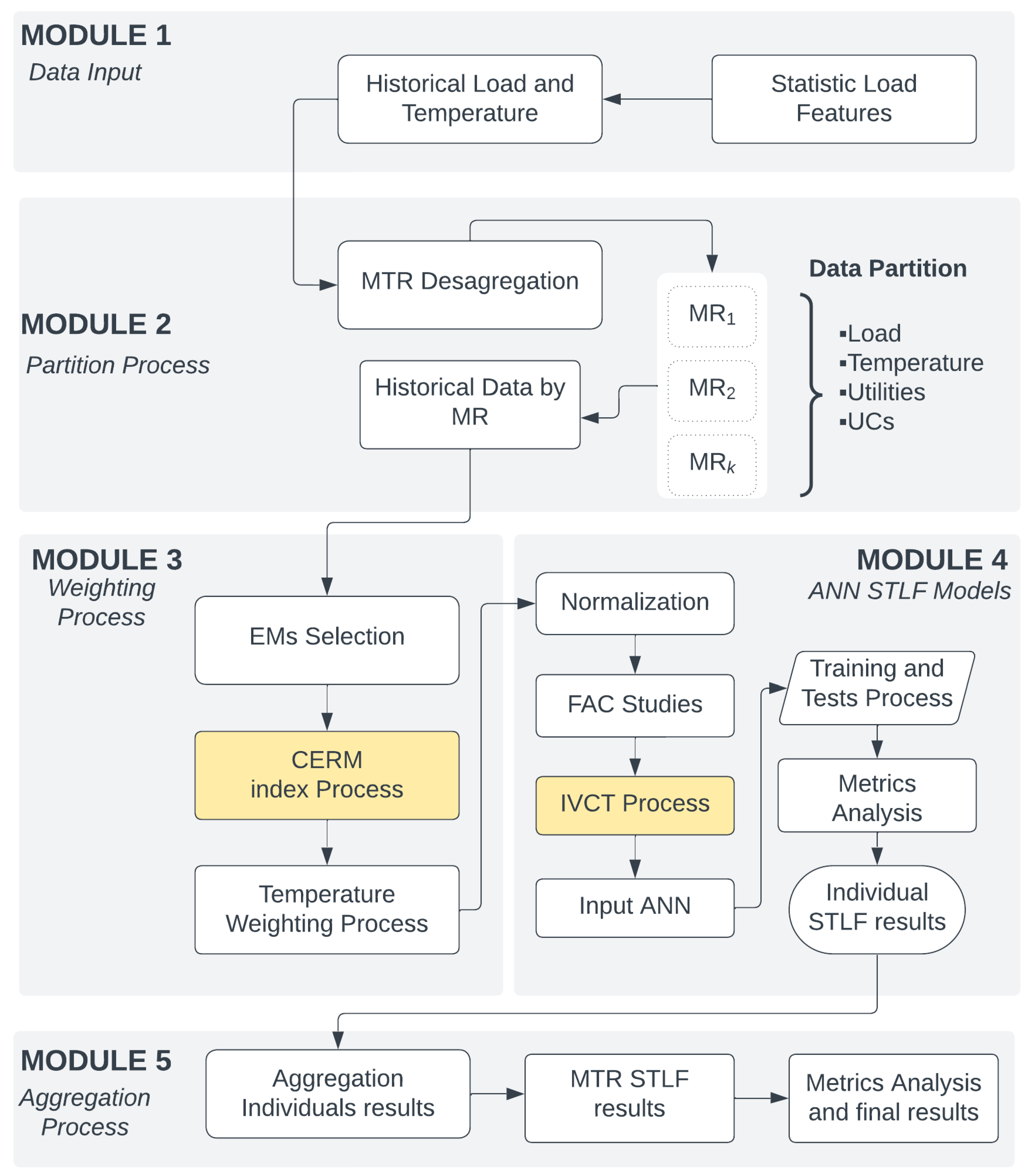
The proposed methodology is elucidated through the flowchart depicted in Figure 1. In Module 1, the Data Input stage encompasses historical load and temperature data, along with pertinent statistical data from the multi-region (MTR), which is crucial for formulating the CERM variable. Subsequently, in Module 2, a partitioning process of the Multi-region (MTR) is conducted, wherein historical demand and temperature data are disaggregated according to the consumption macro-regions (MR k). These macro-regions are defined based on the number of utilities that constitute the MTR.

In Module 3, the weighting step, the meteorological variables of each EM must be weighted before being normalized and used by the prediction model as a single resulting variable. Then, the variable energy consumption by meteorological Region (CERM) is proposed in this work, which represents the contribution of each EM p within the individual MR k and is highlighted in Figure 1.

After the weighting step, Module 4 starts with the normalization process and autocorrelation studies for adjustment of lags for the model training step; that is, both historical load data of each MR k, as well as the already weighted meteorological (temperature) data are analyzed in this step. These data then undergo a training step, such as adjusting the weights and neurons of the ANN model according to the sensitivity studies performed. In addition, this article presents a proposal for the insertion of the variable IVCT, mainly to provide characteristics of load behavior in relation to history and future load. Finally, in Module 5, the hourly and weekly bottom-up STLF is carried out by aggregating the individual forecasts of each MR k. Although the primary emphasis lies in multi-region prediction, this methodology can yield individual forecast outcomes. These individual forecasts can serve as valuable support for numerous studies conducted within each macro-region (MR).

3.1. Multiregion (MTR) Partition Process

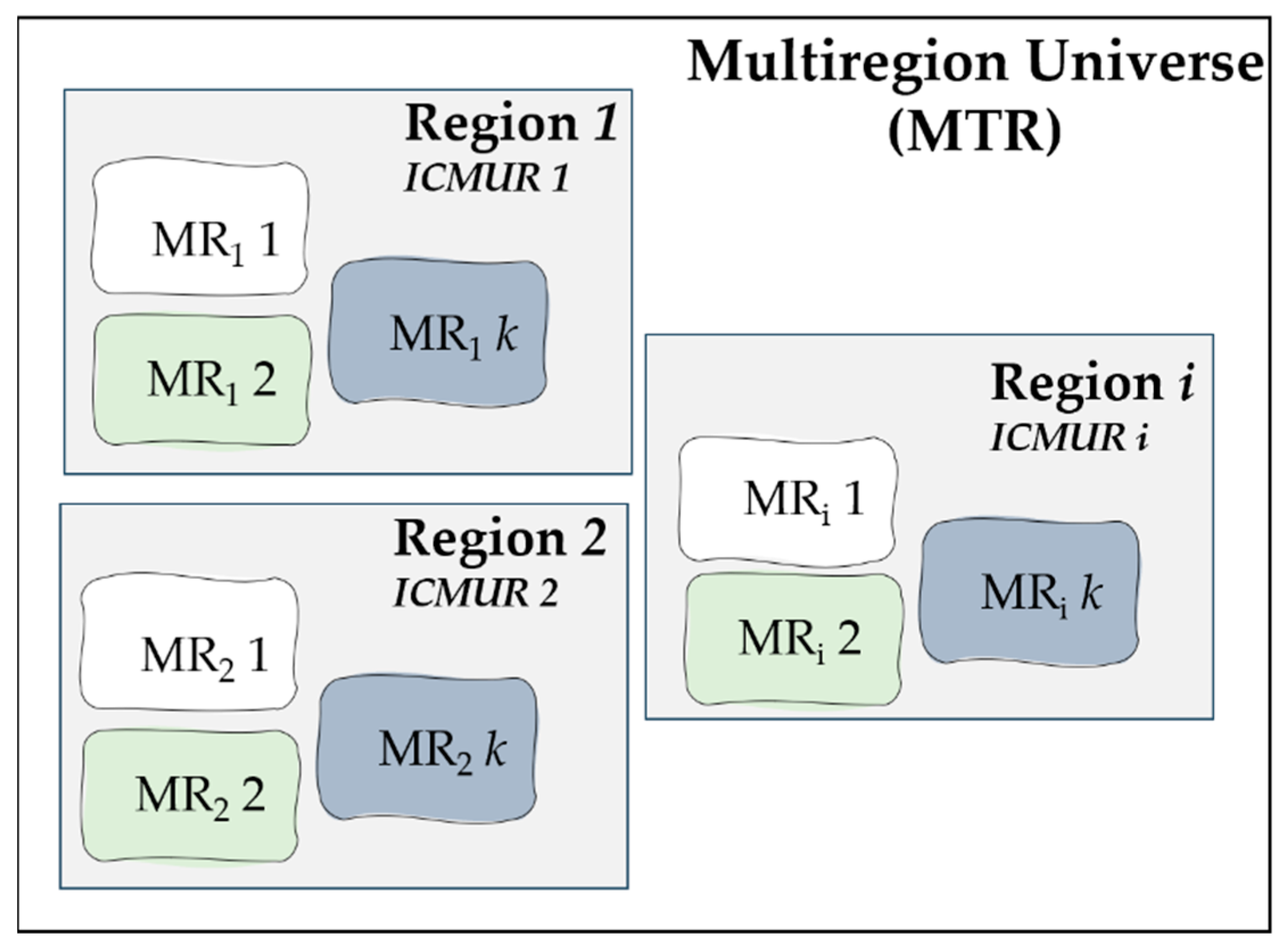
The central focus of the methodology centers around the bottom-up STLF approach. The prediction process involves aggregating the predictions generated by individual models for each macro-region (MR). The composition of a macro-region (MTR) is depicted in Figure 2.

In Figure 2, the analysis universe is the MTR, and Regions 1, 2, …, i represent the i sets belonging to the MTR. Within the Regions set, there are further k subsets, which in this case are the MRs mentioned in the MTR disaggregation step. The objective of this disaggregation is to obtain an individual forecaster for each MR k and then perform aggregation for the MTR forecast. This approach aims to achieve better management of the relationships between load and temperature for load forecasting processing.

3.2. Meteorological Variables Weighting Process

The weighting process is visualized in Figure 3. This flowchart centers around establishing the energy consumption index by meteorological region (CERM), which stands as a significant contribution to this research.

To obtain the CERM index, firstly, the monthly consumption index per regional consumer unit (ICMUR) is calculated. This index is estimated based on the average monthly consumption data and the number of consumers of each region i belonging to MTR. The ICMUR index is calculated using Equation (1).

$${ICMUR}_i=\frac{{CM}_i}{{NUCs}_i}$$

(1)

in which ${CM}_i$ represents the monthly consumption in GWh for the region i belonging to MTR, NUCs_i represents the number of consumers in millions belonging to the region i in analysis. As a result, the ${ICMUR}_i$index is calculated for each region i of MTR given in kWh/(UC.month).

It is observed that each region i of MTR will receive a regional index (ICMUR) according to consumption and number of consumers. This process is carried out as a form of approximation to obtain this same index by MRs.

Within this approach, two scenarios may arise, one where a region comprises a single MR and the other where it encompasses k MRs. In both instances, the MRs take on the ICMUR as ICMU. Consequently, the ICMU index is established for each MR. This index signifies the monthly consumption per consumer unit within the MR and is denoted in kWh/(UC.month). As each MR can have numerous EMs and, consequently, a large volume of available meteorological data, one should identify the number of EMs to be selected for the study. In this article, as a selection criterion, it was adopted to select all available EMs from each MR with valid data in the period considered. To obtain the final index for weighting of EMs, called energy consumption by meteorological region (CERM), Equation (2) applies.

$${CERM}_{EM(p,k)}=ICMU\times {UC}_{EM(p,k)}$$

(2)

where ${CERM}_{EM(p,k)}$ represents the weight given EM p belonging to MR k given in MWh/month; $ICMU$ is fixed and varies according to MR k where is situated EM p. Finally, the variable ${UC}_{EM(p,k)}$ represents the number of consumer units covered by EM p of MR k, given that it provides an estimated energy consumption of the EM region, it was adopted as a region of coverage, the location of the EM city. The final weighting process is carried out by Equation (3).

$${Tp}_{\left(h\right)}=\frac{{\sum }_{p=1}^n{CERM}_{\left(p,k\right)}{T}_{EM(p,h)}}{{\sum }_{p=1}^n{CERM}_{\left(p,k\right)}}$$

(3)

in which ${Tp}_{\left(h\right)}$represents the final weighted average for the meteorological variable in the Hour (h) for the MR k. The variable $T_{EM(p,h)}$represents the variable temperature of each EM p to be weighted hour (h), with the respective weight ${CERM}_{\left(p,k\right)}$. The index (p) depends on the number of selected EMs of each MR k. This weighted average is performed for the entire historical series of meteorological variables used for the training of the model and operation of the same.

3.3. Forecasting Model and Input Variables

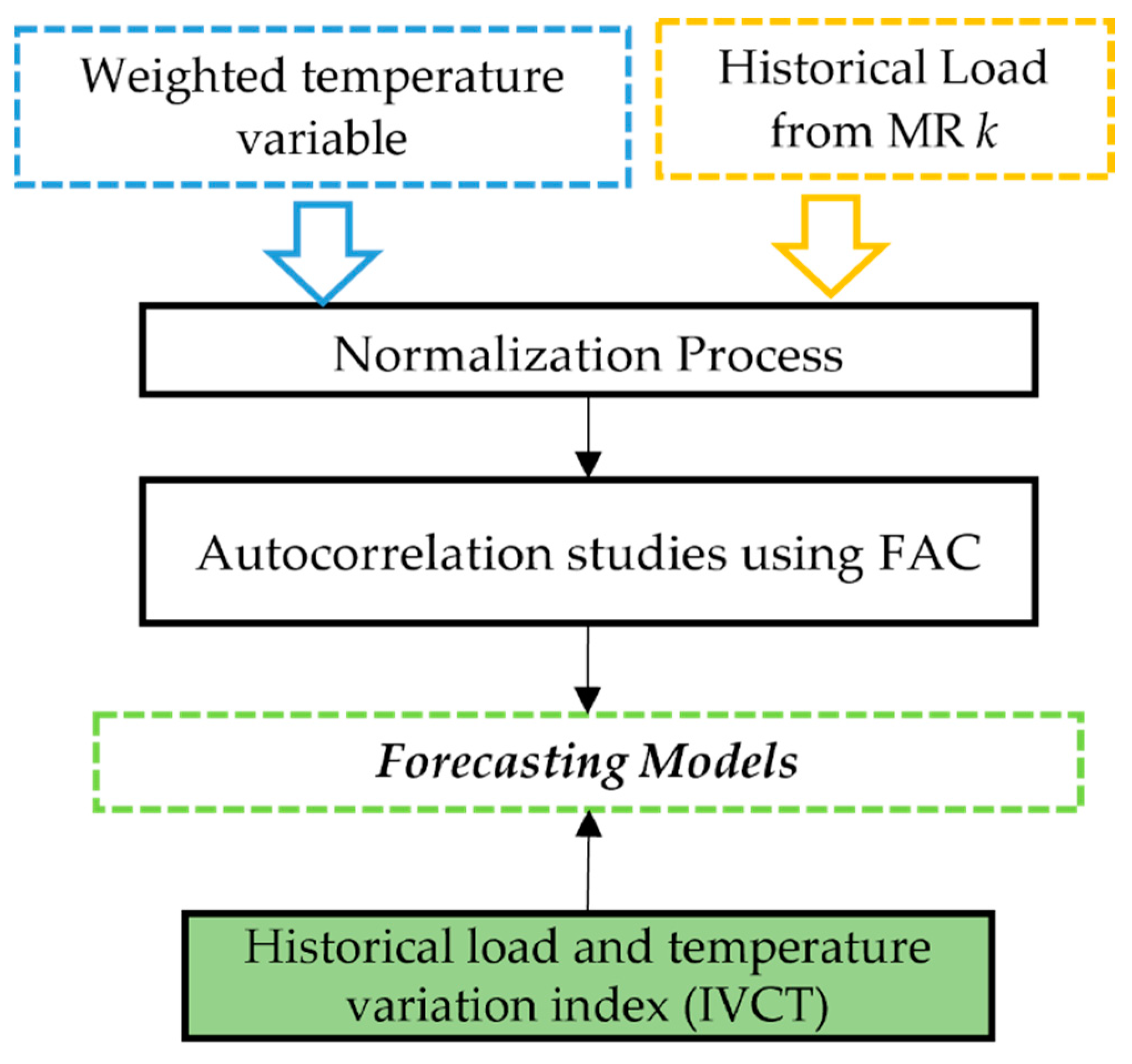
For the elaboration of the load forecasting model, countless characteristics must be defined, such as the technique to be used, training parameters, and choice of variables involved to obtain the Hierarchical Short-Term Load Forecasting. Figure 4 shows all the variables and processes that are involved in defining the models of each MR.

Figure 4 shows that the stage for the definition of the forecasting model for each MR depends on autocorrelation studies of load inputs and weighted meteorological data, which should be normalized before its analysis. In addition, the variable IVCT is proposed in this study.

Within the prediction model, there are still training steps, comprising the definition of the parameters of the applied model as well as the architecture of the ANN used. In addition, in this step, sensitivity analysis of the inputs is performed in order to evaluate different combinations to compose more assertive models for each MR.

3.3.1. Autocorrelation Studies

For the elaboration of any forecasting model, it is necessary to know the relationship between the current and previous observations of a variable that contributes to providing a series of behavior patterns. One of the most popular methods in load prediction is the Autocorrelation Function (FAC) [19]. Consider that $X_t$ is the value observed in time (h) and $\overline{X}$ is the average of the entire analyzed data series (load, for example). The coefficient of autocorrelation $r_d$ that measures the degree of linear correlation between observations separated by delays d is defined by Equation (4) [18]:

$$r_d=r\left(X_t,X_{t-d}\right)=\frac{{\sum }_{t=d+1}^n\left(X_t-\overline{X}\right)·\left(X_{t-d}-\overline{X}\right)}{{{\sum }_{t=1}^n\left(X_t-\overline{X}\right)}^2}$$

(4)

Considering Equation (4), it can be obtained for each lag d, the degree of correlation between the current variable ($X_t$) and the same variable, delayed d lags ($X_{t-d}$). As an exemplification, consider analyzing a lag of 1 h (d = 1). In this case, the coefficient $r_1$is calculated. For d = 2, you have the calculated $r_2$ coefficient, and so on. Each coefficient will range from −1 to + 1, indicating a strong negative or positive correlation. A close to zero $r_d$ value will indicate low or no correlation.

3.3.2. IVCT Index

It’s understood that meteorological conditions, particularly temperature variations, exert substantial influence on load, especially during weekdays. However, during weekends or holidays, a temperature variation might not necessarily result in an impact on energy demand.

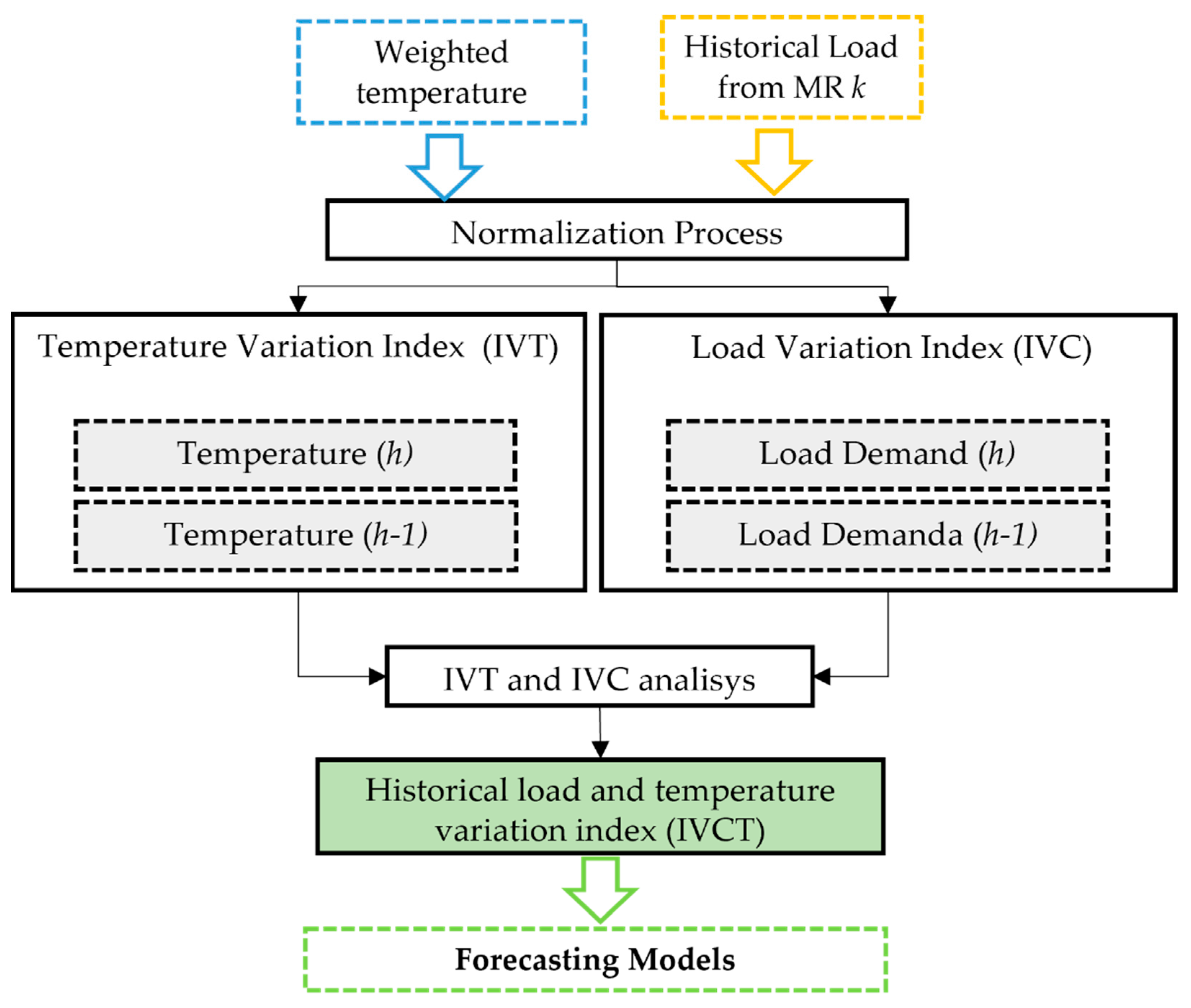
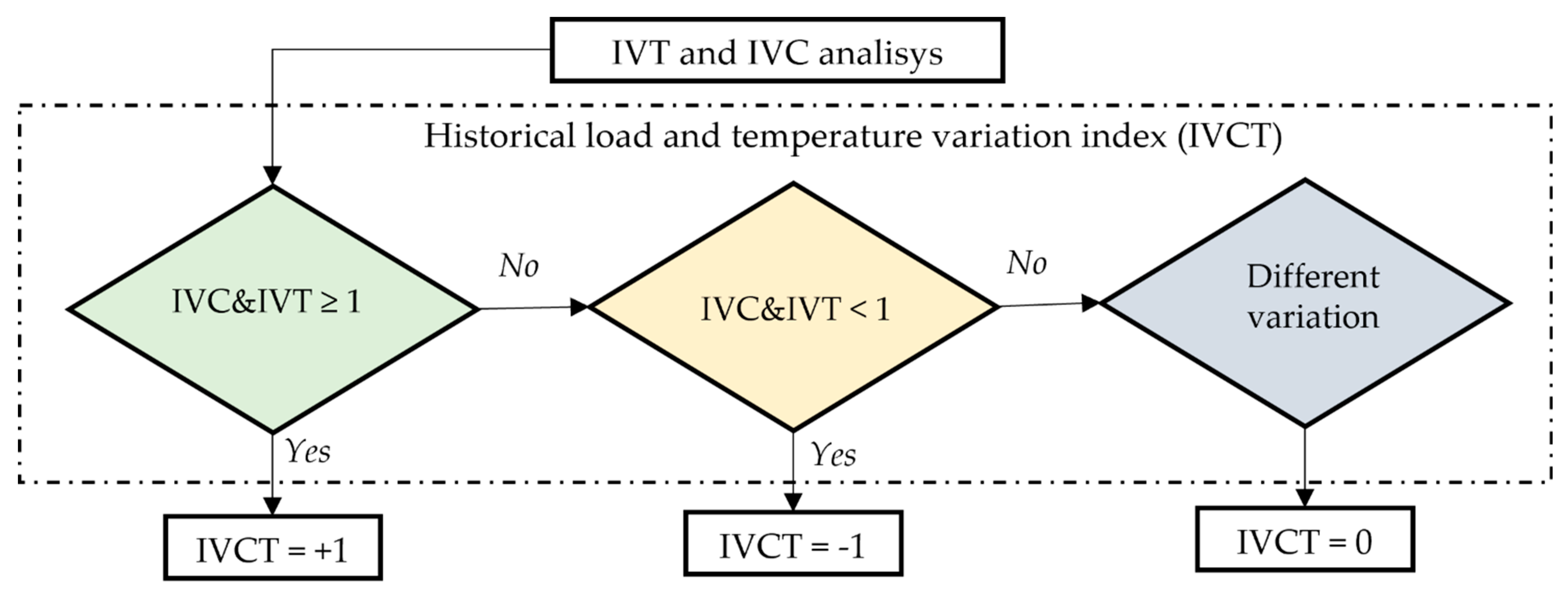
To enhance the understanding of the load forecasting model about load patterns concerning meteorological variables, it is proposed to introduce the historical load and temperature variation index (IVCT). This index is illustrated in the flowchart of Figure 5 and is computed through historical load analysis and temperature weighting. It is then integrated into individual prediction models. While this research focuses solely on temperature as the weighted variable, it is important to note that this weighting methodology can be extended to encompass other meteorological variables.

First, the weighted temperature and hourly demand for MR are normalized [0, 1], and the same ones originate from the steps already processed. Soon after, the load variation index (IVC) and temperature variation (IVT) are calculated for each MR k, according to Equations (5) and (6).

$${IVC}_{(k,h)}=\frac{D_h}{D_{(h-1)}}$$

(5)

$${IVT}_{(k,h)}=\frac{{Tp}_h}{{Tp}_{(h-1)}}$$

(6)

where $D_h$ e ${Tp}_h$ represent the hourly load data and time-weighted temperature (h) and $D_{(h-1)}$and ${Tp}_{(h-1)}$the referred data to the previous hour (h − 1). The result of this division will result in a value greater or lesser than 1 (Figure 6). For example, in case the current demand ($D_h$) is greater than previously occurred ($D_{(h-1)}$), so the result of Equation (5) will result in a greater value than 1 since there has been an increase in demand. Otherwise, it will receive a value less than 1. The same analysis is valid for the IVT index.

The results of IVT and IVC are subsequently compared to assess whether historical temperature variations correspond to historical load variations or not. If both indexes have values greater than 1, then IVCT will receive the value +1, as depicted in Figure 6 for the first condition. In such cases, it is estimated that an increase in temperature corresponds to an increase in load. Conversely, if IVT and IVC have values lower than 1, IVCT will assume the value −1, indicating that both load and temperature have decreased. The final condition addresses the situation where IVC and IVT variations are contradictory; if demand decreases while temperature rises, the IVCT variable will be assigned a weight of zero.

Table 2. IVTC weight according to IVT and IVC values.

IVT Values	IVC Values	IVTC Weight
$\ge$1	$\ge$1	+1
<1	<1	−1
$\ge$1	<1	0
<1	$\ge$1	0

summarizes these conditions.

3.3.3. Forecast Models

As observed in [6], a great number of techniques have been employed for short-term load forecasting. However, artificial intelligence techniques (AI) stand out for their potential in load modeling. Among the AI methods currently applied are Artificial Neural Networks (ANNs), Fuzzy Logic, Neuro-Fuzzy Adaptive Systems, Genetic Algorithms (GAs), and Support Vector Machines (SVMs) [30,31,32].

In this context, ANN constitutes a highly prevalent technique within short-term load forecasting [33]. Specifically, the Multi-Layer Perceptron (MLP) Feed-Forward [34,35] architecture was adopted for this work. Furthermore, in [10], the authors emphasize that the ability to generalize and capture complex non-linear relationships makes ANNs highly attractive for load forecasting problems.

In summary,

Table 3. Input basic parameters to the ANN module.

Input Variables	Description
Month of Year	Dummy numeric variable (Jan. = 1, Feb. = 2, …, Dec. = 12)
Hour of the Day	Dummy numeric variable (0 to 23)
Day of the Week	Dummy numeric variable (Mon. = 1, Tue. = 2, …, Sun. = 7)
Data Lags	Autocorrelation studies per MR 1
IVCT	Variable proposed

¹ According to FAC studies.

presents the ANN-MLP base inputs to the load forecasting model proposed. The entries with lags will depend on the autocorrelation study for each MRhe. The utilization of dummy variables is notable, as they define the nature of inputs to be integrated into the forecasting model. These variables are employed to represent daily, weekly, and monthly seasonality patterns, which are then incorporated into the prediction models [26,27].

Table 4. ANN parameters applied to the hierarchical STLF models.

Parameter	Value
Hidden layer number	1
Hidden layer neurons	10 to 50
Output neurons	1
Hidden layer activation function	Log-sigmoid
Output layer activation function	Linear
Training Algorithm	Levenberg–Marquardt
Training data partition	75%–25%–0%
Epochs	1000

shows the main ANN parameters applied to network structure and training. It’s important to note that all parameters are employed for initializing the prediction models, and default MATLAB parameters have been adopted. The only parameter subject to variation is the “Hidden layer neurons”, which vary depending on the neural network training algorithm.

Following the standardization of the input pattern, the process involves initializing the Artificial Neural Network (ANN) and establishing the initial training parameters. This is carried out in accordance with the flowchart presented in Figure 7.

After defining these parameters, the training process is initiated for each MR k, considering an initial number of neurons in the intermediary layer. Based on this initial number, the process of training, verification, and testing by n iterations is performed. It was initially defined as 30 iterations for each I neurons of the middle layer.

Metrics for Evaluation of the Model

It is important to recognize that prediction models utilizing Machine Learning (ML) methods, like Artificial Neural Networks (ANN), are developed using a particular dataset. As a result, the dataset’s origin, quality, and size are shaped by the specific problem being studied. This also extends to considerations such as the level of detail in time series data and the chosen sampling approach [35]. This variety in data characteristics presents a complex challenge when it comes to comparing ANN models. Depending on data availability, various approaches can be explored to evaluate how well the classifier performs on unseen data. As a result, instead of directly comparing results with other methods, metrics such as MAPE, MAE, and RMSE are commonly utilized as reference points for the evaluation and comparison of the model. It is crucial to emphasize that the primary objective of our research is to enhance the accuracy of the forecast model through the weighting process and the introduction of a new variable for load forecasting over a large geographical area. In this context, the evaluation strategy for error metrics involved comparing the use of these variables within the same neural network model with a model that excludes any meteorological or weighting variables.

In this sense, according to the simulation results for each iteration, the prediction efficiency is verified using the Mean Absolute Percentage Error (MAPE) between the $x_j$ observed loads and those estimated in the forecast $y_j$. The MAPE is defined by Equation (7).

$$MAPE\left(\%\right)=\frac{100}{N}\sum _{j=1}^N\frac{\left|x_j-y_j\right|}{x_j}$$

(7)

where N depends on the forecast horizon (daily MAPE, in this case, N = 24, or weekly MAPE N = 168). As this is a short-term forecast, it was considered a maximum horizon of one week ahead with hourly and daily discretization. The prediction window is always shifted as new data is provided to the network and must be retrained for a new forecast period.

For each set of interactions for i neurons minimum MAPE is stored until the maximum number of neurons specified is reached. When reaching the maximum number of neurons, the simulation result that obtains the smallest MAPE will be considered for the MR k, which in this case is called Global MAPE. It is also important to highlight that, as part of the training process, sensitivity analysis is conducted by combining input variables to attain the ultimate network for each MR k. Following these steps, performance metrics, including Mean Absolute Error (MAE) and Root Mean Squared Error (RMSE), are calculated based on Equations (8) and (9). These metrics are widely used in the literature [36].

$$MAE=\frac{1}{N}\sum _{j=1}^N\left|x_j-y_j\right|$$

(8)

$$RMSE=\sqrt{\frac{1}{N}\sum _{j=1}^N{\left(x_j-y_j\right)}^2}$$

(9)

where N represents the number of predicted values, $y_j$ is the predicted value and $x_j$ is the actual value which corresponds to the predicted value.

3.3.4. Aggregation Process for Bottom-Up STLF

Obtaining the forecast for MTR is accomplished by aggregating the individual forecasts of each MR k that resulted in lower Global MAPE. Before performing the aggregation, the data are denormalized and then aggregated, according to Equation (10).

$${PMTR}_{\left(j\right)}=\sum _{k=\mathrm{1,2},3,\dots }^{kmáx}{PMR}_{(k,h)}$$

(10)

in which ${PMTR}_{\left(j\right)}$ represents the hourly multiregion forecast for the MTR for the N horizon of forecast. The PMTR considers the sum of the individual estimates of each MR k, called the ${PMR}_{(k,h)}$.

It is noteworthy that besides this methodology providing the aggregate multiregional forecast, one can still obtain the individual prediction of each MR belonging to MTR and may assist in various planning activities within each MR. This process is repeated by the Other MTRs, who possess k MRs.

4. Results and Discussion

4.1. Assumptions for Characterization of the Case Study

For the proposed methodology and validation, a case study is composed of the Brazilian South Region electrical subsystem. The South MTR is composed of three regions, subdivided into five MRs (Utilities), MRs 3, 4, and 5 belonging to the same province. The main characteristics of MRs are shown in

Table 5. Characterization of South MTR.

Parameters	MR1	MR2	MR3	MR4	MR5
Region	1	2	3	3	3
Mean Temperature Range for the Summer (°C) 1	23	23.1	27.9	30.3	27.3
Mean Temperature Range for the Winter (°C) 1	27.2	26.5	30.4	32.4	29.3
Loadmin (MW)	2071	1456	568	567	1456
Loadmax (MW)	5127	4127	1937	1967	1920
Area (km2)	180.0	95.3	90.7	99.5	73.6
NUC (milions)	4.4	2.8	1.4	1.3	1.6
EMs	21	19	14	9	10

¹: Source: INMET, Instituto Nacional de Meteorologia. Available online: http://www.inmet.gov.br/portal/index.php?r=estacoes/estacoesautomaticas (accessed on 20 August 2023).

.

In order to evaluate the forecasting models for each MR, the dataset was partitioned into two training sets: the first one (C1) comprised 1 June 2012 to 8 July 2013, and the second (C2), from 1 October 2012 to 4 November 2013. This partition was adopted to evaluate the robustness of the models in different periods of demand and temperature of each MR. For the first set, called Set 1 (C1), the tests are conducted to predict the period from 9 July to 5 August 2013, which refers to the winter season for MRs. For the second set of tests, called Set 2 (C2), the forecast is made for the period from 5 November to 2 December 2013, corresponding to the spring period in the region. It is noteworthy that the prediction is carried out with a 7-day horizon, with daily and hourly discretization. With each simulation window offset (7-day window), new data are entered for retraining of the new network.

In addition to the fixed pattern of the input data, highlighted in Table 3, for each set of tests, sensitivity analyses are performed, highlighted in

Table 6. Sensitivity analyses to the ANN module.

Input Variables	Description
S1	Test considering only IVCT variable
S2	Test considering only weighted temperature with CERM
S3	Test considering only load demand

.

The demand data originated from the historical base of the National Electrical System Operator of Brazil (ONS), and the temperature data were obtained through the history of reading automatic meteorological stations (EMs) belonging to the National Institute of Meteorology (INMET) [3].

The methodology was implemented within the MATLAB environment on a workstation equipped with an Intel(R) Core(TM) i7-5500U CPU running at 2.4 GHz, 8 GB of RAM, and utilizing the Microsoft Windows 10 operating system.

4.2. Analysis of MR Prediction Results

Based on the methodology described, South MTR is partitioned, and MRs are selected for short-term forecasting, with demand data imported from the database and normalized. In the weighting step, it is first calculated according to Equation (1), the ICMUR index by region, shown in

Table 7. ICMU process.

Region	Electricity Consumption (GWh/month)	UCs	ICMUR (kWh/(UC.Month)
1	2.4786	4,650,487	532.97
2	1.9208	7,121,656	269.70
3	2.4350	6,020,604	404.44

.

After calculating the ICMUR by region, the ICMU index is obtained according to the region where each MR is located. Finally, the CERM index is calculated for each EM according to Equation (2). This index is then used for weighting each EM according to Equation (3).

Shortly after this weighting, the variable IVCT is calculated according to the flowchart in Figure 6 and Equations (5) and (6). Finally, the autocorrelation analysis is performed, according to Equation (4), to identify the most representative lags for the demand and temperature of MRs.

Table 8. Representative demand lags after autocorrelation studies.

MR	r1	r24	r168	r336
1	0.9426	-	0.8991	0.8620
2	0.9586	-	0.8867	0.8395
3	0.9386	-	0.8983	0.8697
4	0.9474	-	0.8619	0.8197
5	0.9422	0.8619	0.8642	-

shows the demand lags that will compose the model entry pattern of MRs.

For the variable weighted temperature, the same procedure was performed, and the lags 1 and 2 were the most representative of the coefficient presented; that is, the temperatures will be used 1 and 2 h before the prediction.

Based on the training performed,

Table 9. Prediction results for each MR considering lowest monthly MAPE.

Set of Tests	Type of Day	Sensitivity Test	MR1	MR2	MR3	MR4	MR5
C1	Weekday	S1	2.39	2.33	2.46	2.58	2.21
		S2	2.33	2.55	2.51	2.74	2.31
		S3	2.12	2.35	2.52	2.80	2.35
	Weekend	S1	3.20	3.84	3.88	3.80	2.61
		S2	3.05	4.26	4.06	3.91	3.01
		S3	3.20	4.11	4.1	3.55	2.98
C2	Weekday	S1	2.16	2.62	2.16	2.63	2.36
		S2	2.09	3.03	2.05	2.65	2.36
		S3	2.20	3.30	2.09	2.83	2.62
	Weekend	S1	3.11	3.56	3.87	3.67	2.82
		S2	3.38	3.53	3.86	4.14	2.84
		S3	3.10	3.79	3.90	4.16	3.07
	Holidays	S1	3.81	2.97	4.86	5.41	4.85
		S2	4.79	4.21	5.84	7.19	5.78
		S3	5.75	5.16	6.42	7.48	5.85

shows the prediction results for each MR that obtained the lowest mean monthly MAPE for C1 and C2.

Table 9 shows that the variable S1 (only IVCT variable) demonstrated the best performance in the sensitivity analysis, occurring in 68% of the test sets, based on the average Mean Absolute Percentage Error (MAPE). When considering the isolated use of the demand variable (S3), a higher MAPE was found in only 12% of the tests. This outcome could potentially be attributed to varying correlations between temperature and demand in each test period [21]. Furthermore, it is important to observe that variable S2 (CERM) also exhibited a favorable performance, occurring in 20% of the simulated cases. This further underscores the contribution of the variables proposed in this article.

4.3. Global Prediction Analysis

After obtaining individual predictions for each MR, the aggregation step is executed to create the overall load forecast for the South MTR. This aggregation process is carried out using Equation (10), which involves summing the daily estimates in megawatts (MW) from the models for each MR.

As a criterion for comparing the proposed model, a forecasting model was elaborated considering the total aggregate demand of the South MTR, called the Aggregate Prediction Model (AP). The elaboration of this model followed the same proposed training assumptions with the same training window and the same ANN MLP technique. The aggregate model input pattern uses only normalized demand data. The results derived from this model are described as MAPE_AP1 and MAPE_AP2, corresponding to the results for sets C1 and C2, respectively.

Table 10. MAPE performance to proposed model and AP model.

Day	MAPEC1(%)	MAPEAP1(%)	MAPEC2(%)	MAPEAP2(%)
Tuesday	0.72	1.19	0.75	1.33
Wednesday	0.75	1.17	0.72	1.34
Thursday	0.79	1.20	0.74	1.16
Friday	0.64	1.06	0.62	1.32
Saturday	0.74	1.02	0.67	1.07
Monday	0.83	1.29	0.86	1.27
Sunday	0.64	1.14	0.82	1.26
Average	0.73	1.15	0.74	1.25
Holiday	-	-	1.07	2.60

displays the average Mean Absolute Percentage Error (MAPE) for each day of the week in Sets C1 and C2.

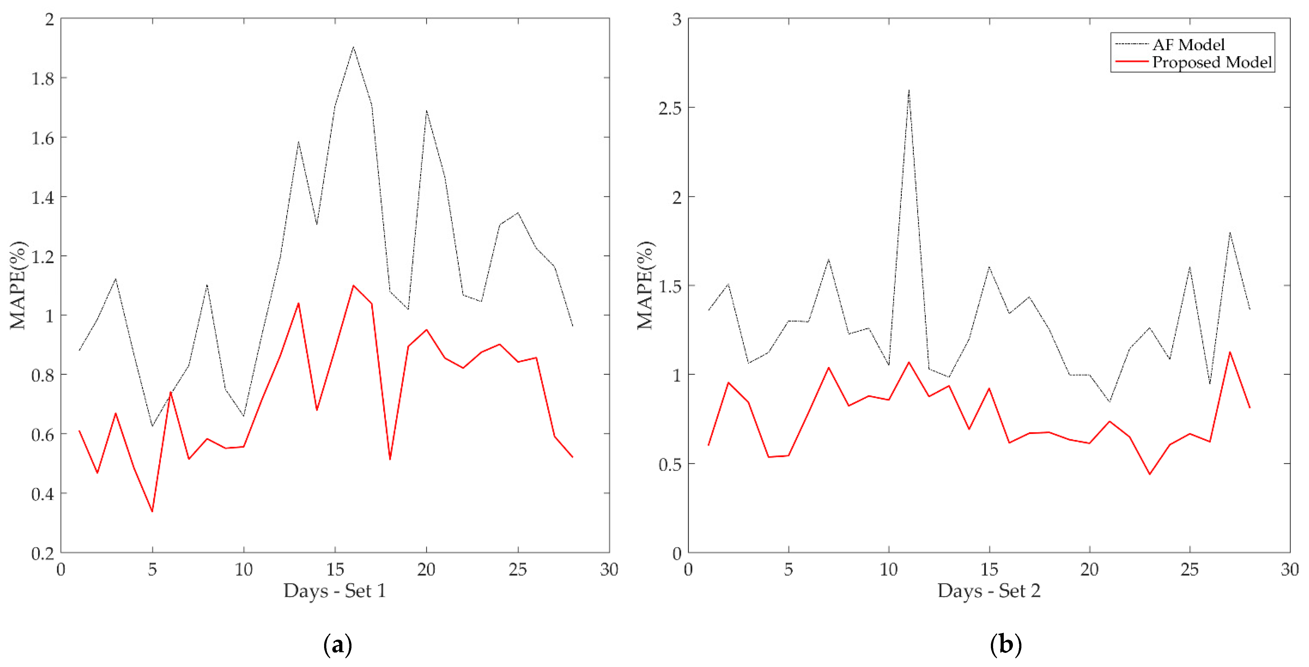
Table 10 shows that the proposed methodology presented a superior performance in relation to the aggregate model for weekdays and weekends. For example, the MAPE found between the Thursdays of Set C1 was 0.79% and 1.20% for the proposed model and AP model, respectively. In Figure 8, the results also demonstrate the efficiency of the proposed model compared to the aggregated model in terms of average daily MAPE for periods C1 (a) and C2 (b).

It can be observed that the proposed methodology presented lower errors in both test datasets (continuous red line). For the holiday (peak in Set C2), the proposed methodology obtained a MAPE of 1.07% in relation to the 2.60% obtained by the AP model.

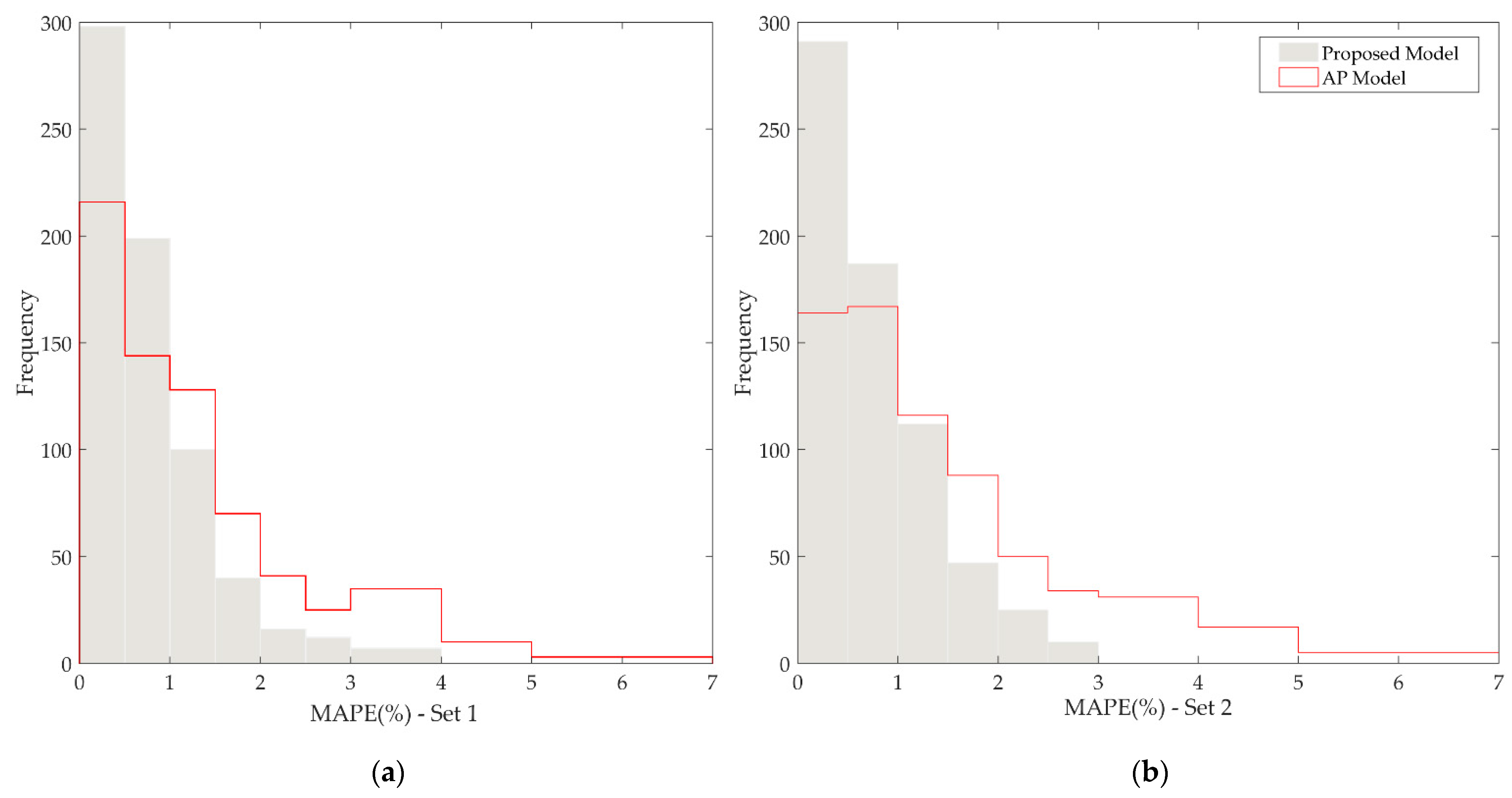
To analyze the distribution of the time-based Mean Absolute Percentage Error (MAPE) for both models, Figure 9 illustrates a comparison between the MAPE distributions for sets C1 (a) and C2 (b), respectively. The height of the bars on the y-axis reflects the frequency of time-based errors observed within the test sets, while the average range of errors is indicated on the x-axis.

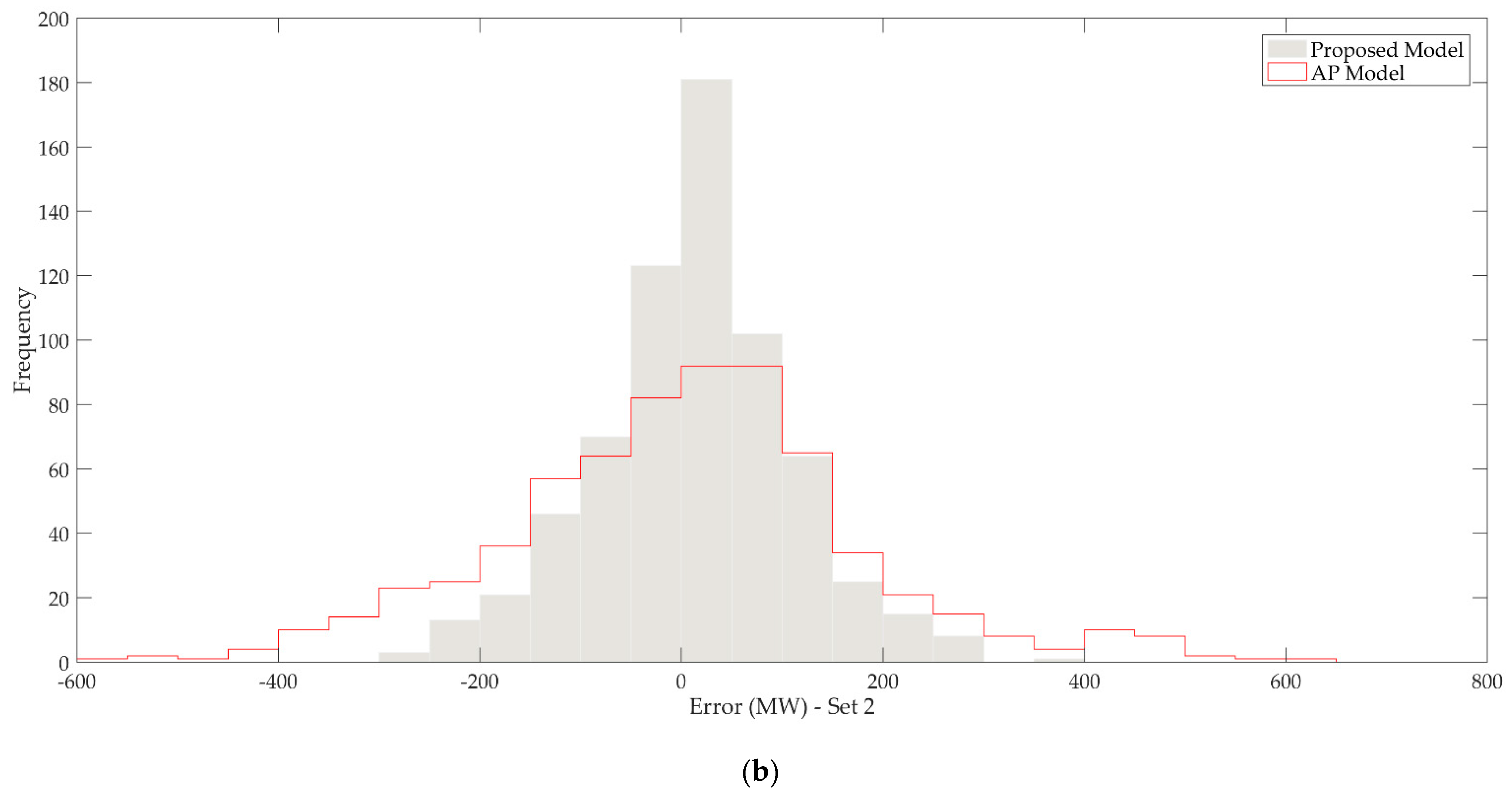
It is observed in Figure 9 that for both sets of simulation, there is a higher concentration of errors, less than 1% for the proposed model than for the AP model. It is also noted that errors greater than 2% occurred more frequently for the AP model, thus corroborating the efficacy of the methodology proposed in this article with respect to performance in both sets of tests. Figure 10 depicts the distribution of load forecast errors in MW for each dataset.

It can be noticed that for the proposed model, there is a higher concentration of prediction errors in the 100 MW range for both datasets, represented by the peaks in the histograms. Moreover, it is observed that there is a higher dispersion of errors for the aggregated model. This dispersion of errors is reflected in the average MAE and RMSE results of the models, as shown in

Table 11. MAE and RMSE performance to proposed model and AP model.

	Proposed Model				AP Model
Type of Day	C1		C2		C1		C2
	MAE	RMSE	MAE	RMSE	MAE	RMSE	MAE	RMSE
Tuesday	76.40	103.34	82.50	107.45	129.54	163.74	147.35	183.24
Wednesday	80.35	102.68	78.09	96.27	127.15	161.72	150.86	190.97
Thursday	84.93	106.89	81.89	101.38	127.73	165.08	130.16	173.56
Friday	67.98	87.02	68.18	88.02	110.32	144.13	147.68	179.85
Saturday	67.83	94.69	61.12	85.31	93.06	130.60	99.62	139.56
Monday	62.83	78.91	69.76	87.82	96.53	129.08	104.48	137.21
Sunday	64.49	84.95	86.96	108.36	120.99	164.16	135.77	183.61
Mean	72.12	94.07	75.50	96.38	115.05	151.22	130.84	169.71

.

The results in Table 11 reveal that the proposed model demonstrated superior performance for both analyzed metrics. For instance, the average RMSE obtained for Set C2 was 169.71 MW for the AP model and 96.38 MW for the proposed model, respectively. This dispersion is detailed in

Table 12. Load forecasting error type.

Set of Tests	Type of Error	Proposed Model	AP Model
		<100 MW	<100 MW
C1	Underestimation (+)	75%	60%
	Overestimation (−)	79%	56%
C2	Underestimation (+)	71%	52%
	Overestimation (−)	70%	46%

, where the concentration of positive errors (under-forecasting) and negative errors (over-forecasting) within the 100 MW range is displayed.

It is possible to observe in Table 12 that the proposed model exhibited a concentration of under-forecasting and over-forecasting errors above 70%, up to 100 MW, in contrast to the aggregated model, which resulted in a greater dispersion of errors, as evidenced by errors exceeding 100 MW. This information, coupled with the other presented results, highlights the efficiency and applicability of the model for hierarchical load forecasting in large geographical areas and its potential for various studies within the Power Systems.

5. Conclusions

This work presented the development of a methodology as a contribution to hierarchical short-term load forecasting. The approach sought to contribute to the elaboration of models for macro-regions of consumption where there is the challenge of realizing the global prediction of a system with a large territorial dimension and weather diversity.

As part of the methodology, the proposed multi-regional prediction seeks to partition an MTR in macro-regions, perform the individual prediction of each MR, and finally aggregate the forecasts to compose a global model with greater assertiveness. This partition aims to reduce the granularity of the characteristics of the MR as to the extent and temperature variations. These variations in temperature along the territory of the MR, and its influences on the aggregate demand of the MR lead to the main contribution of this work.

In this sense, the index CERM was proposed, which is responsible for providing a weight related to the Average Consumption of the region covered by the EM in relation to their contribution to the aggregate demand of the MR.

The results were evaluated considering two sets of tests, with the same training window, but in winter periods (Set C1) and spring (Set C2). Sensitivities analyses were performed, proposing different combinations among the revolving as a way to evaluate the best performance for each MR in the case of the methodology proposed in this work.

As for the simulation results, it was observed that the proposed IVCT index presented the best average performances for the MRs in the periods of analysis.

Shortly after the individual forecasts, the MTR forecast is carried out through the aggregation of the best-performing predictor models of each MR. Through this approach, a mean MAPE of less than 1% was obtained for sets 1 and 2, showing superior performance to the AP model. Moreover, when analyzing the MAE and RMSE metrics for both datasets, it is evidenced that the AP model showed a higher dispersion of load forecasting error.

Finally, the approach proposed in this article proved to be efficient in the prediction of multiregional load, providing an estimate of the load with reduced error and can be applied with satisfactory performance for such problems.