


New Feature Selection Approach for Photovoltaïc Power Forecasting Using KCDE


Abstract
1. Introduction
2. Data
2.1. Historical PV Power Production Data
2.2. WRF Outputs
3. Methods
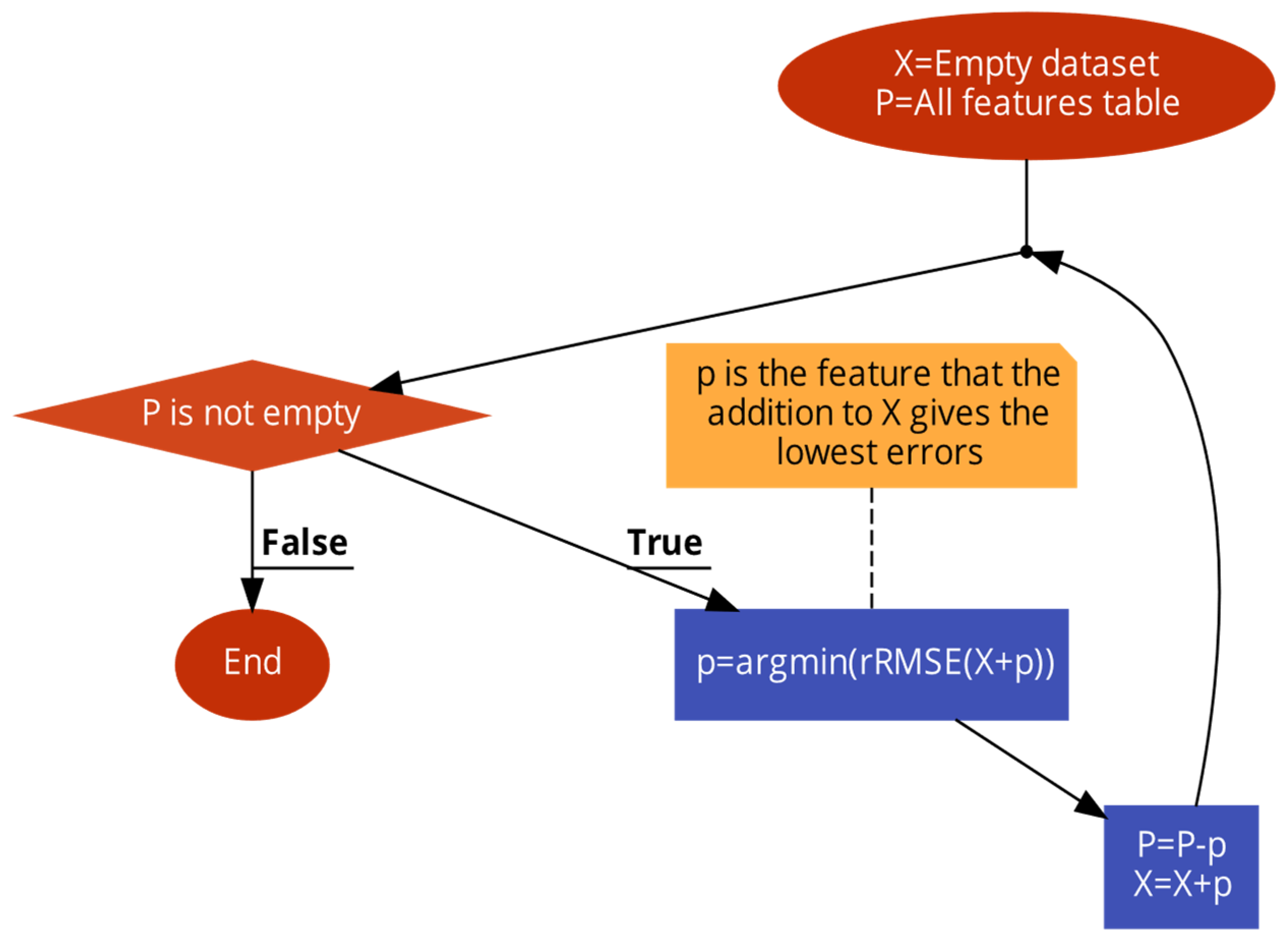
3.1. SFS
3.2. KDCE
3.3. Linear Regression
3.4. Pearson Correlation
3.5. RReliefF
4. Results and Discussion
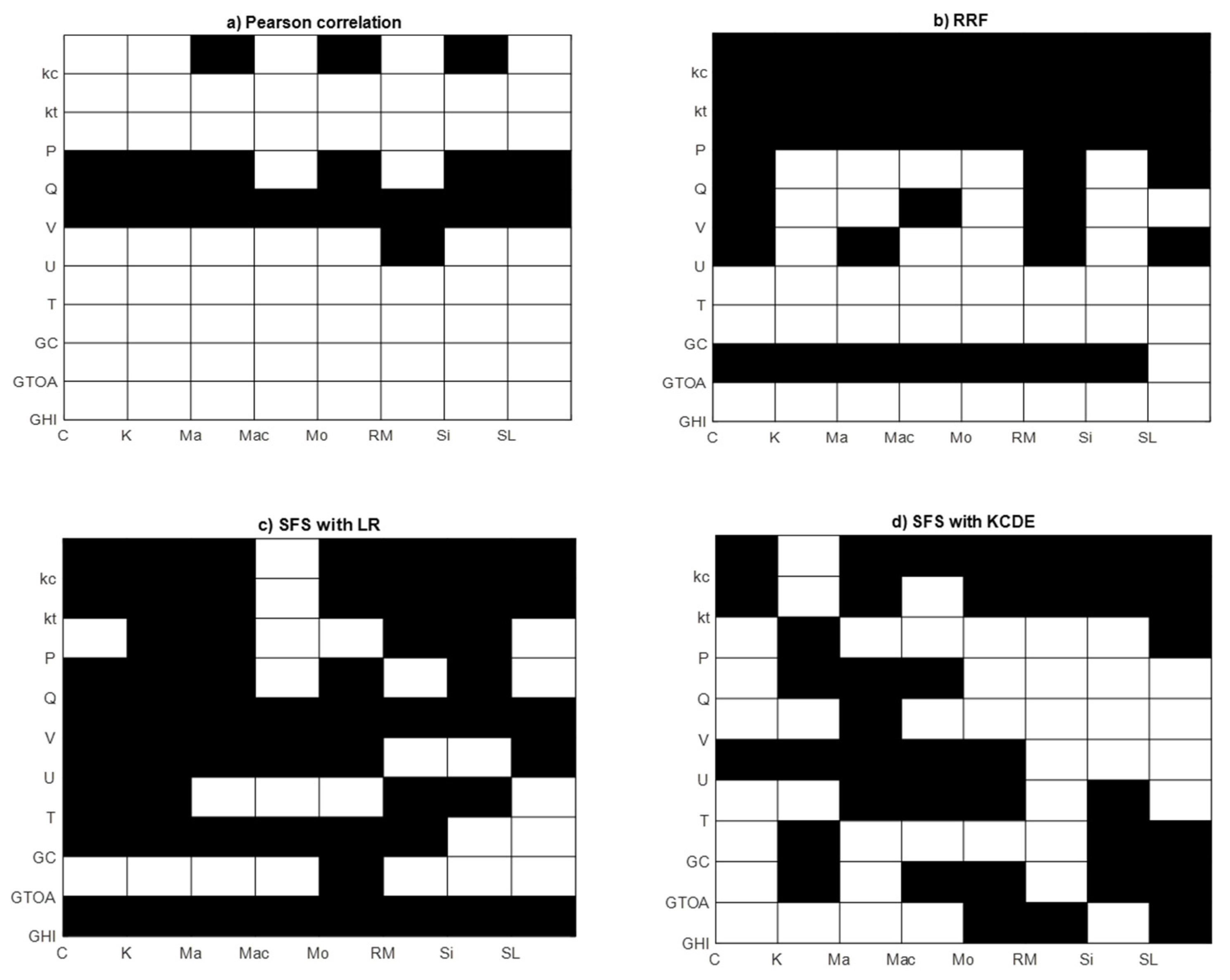
4.1. Features Selected by Each FS Method
4.2. Comparison between Forecasting Errors for Each FS Method
5. Conclusions
- SFS-KCDE is an adequate FS method as it improves forecast accuracy for clear and overcast sky conditions.
- Wrapper methods, like SFS-KCDE, show better forecasting performance than the filter methods and should be used.
- SFS-KCDE can face non-linear problems, as it outperformed other FS methods, including SFS-LR, for overcast hours.
- FS is an essential point of solar forecasting as it improves the forecast accuracy for most cases.
Author Contributions
Funding
Data Availability Statement
Acknowledgments
Conflicts of Interest
Nomenclature
| Abbreviations | |
| PV | Photovoltaïc |
| KCDE | Kernel Conditional Density Estimator |
| FS | Feature selection |
| SFS | Sequential Forward Selection |
| SBS | Sequential Backward Selection |
| RRF | RReliefF |
| WRF | Weather Research and Forecasting |
| ANN | Artificial Neural Network |
| PHANN | Physical and Artificial Neural Network |
| ITCZ | Inter Tropical Convergence Zone |
| NWP | Numerical Weather Prediction |
| PCA | Principal Component Analysis |
| LR | Linear regression |
| SFS-LR | SFS with linear regression as a prediction model |
| SFS-KCDE | SFS with KCDE as prediction model |
| GFS | Global Forecasting System |
| IFS | Integrated Forecast System |
| UCAR | University Corporation for Atmospheric Research |
| Symbols | |
| n | Amount of data |
| r | Pearson correlation index |
| rRMSE | Relative root mean squared error |
| rMBE | Relative mean bias error |
| rMAE | Relative mean absolute error |
| kc | Clear sky index |
| SZA | Solar zenith angle |
| Cos(SZA) | Cosinus of solar zenith angle |
References
- Sobri, S.; Koohi-Kamali, S.; Rahim, N.A. Solar photovoltaic generation forecasting methods: A review. Energy Convers. Manag. 2018, 156, 459–497. [Google Scholar] [CrossRef]
- IEA. Renewables 2019. Available online: https://www.iea.org/reports/renewables-2019 (accessed on 10 February 2020).
- Castangia, M.; Aliberti, A.; Bottaccioli, L.; Macii, E.; Patti, E. A compound of feature selection techniques to improve solar radiation forecasting. Expert Syst. Appl. 2021, 178, 114979. [Google Scholar] [CrossRef]
- IEA. World Energy Outlook 2020; IEA: Paris, France, 2020. Available online: https://www.iea.org/reports/world-energy-outlook-2020 (accessed on 18 January 2021).
- Notton, G.; Nivet, M.-L.; Voyant, C.; Paoli, C.; Darras, C.; Motte, F.; Fouilloy, A. Intermittent and stochastic character of renewable energy sources: Consequences, cost of intermittence and benefit of forecasting. Renew. Sustain. Energy Rev. 2018, 87, 96–105. [Google Scholar] [CrossRef]
- Kreuwel, F.P.; Knap, W.H.; Visser, L.R.; van Sark, W.G.; de Arellano, J.V.-G.; van Heerwaarden, C.C. Analysis of high frequency photovoltaic solar energy fluctuations. Sol. Energy 2020, 206, 381–389. [Google Scholar] [CrossRef]
- Denholm, P.; Margolis, R.M. Evaluating the limits of solar photovoltaics (PV) in traditional electric power systems. Energy Policy 2007, 35, 2852–2861. [Google Scholar] [CrossRef]
- Adewuyi, O.B.; Lotfy, M.E.; Olabisi Akinloye, B.; Howlader HOr, R.; Senjyu, T.; Narayanan, K. Security-constrained optimal utility-scale solar PV investment planning for weak grids: Short reviews and techno-economic analysis. Appl. Energy 2019, 245, 16–30. [Google Scholar] [CrossRef]
- Pérez-Arriaga, I.J.; Batlle, C. Impacts of Intermittent Renewables on Electricity Generation System Operation. Econ. Energy Environ. Policy 2012, 1, 3–18. [Google Scholar] [CrossRef]
- Batlle, C.; Rodilla, P. Generation Technology Mix, Supply Costs, and Prices in Electricity Markets with Strong Presence of Renewable Intermittent Generation; IIT Working Paper IIT-11-020A; Institute for International Trade: Adelaide, Australia, 2011. [Google Scholar]
- Rehman, S.; Bader, M.A.; Al-Moallem, S.A. Cost of solar energy generated using PV panels. Renew. Sustain. Energy Rev. 2007, 11, 1843–1857. [Google Scholar] [CrossRef]
- Majdi, A.; Alqahtani, M.D.; Almakytah, A.; Saleem, M. Fundamental Study Related to The Development of Modular Solar Panel for Improved Durability and Repairability. IET Renew. Power Gener. (RPG) 2021, 15, 1382–1396. [Google Scholar] [CrossRef]
- Soubdhan, T.; Abadi, M.; Emilion, R. Time Dependent Classification of Solar Radiation Sequences Using Best Information Criterion. Energy Procedia 2014, 57, 1309–1316. [Google Scholar] [CrossRef]
- Visser, L.; AlSkaif, T.; van Sark, W. Operational day-ahead solar power forecasting for aggregated PV systems with a varying spatial distribution. Renew. Energy 2022, 183, 267–282. [Google Scholar] [CrossRef]
- Van Der Meer, D.W.; Widén, J.; Munkhammar, J. Review on probabilistic forecasting of photovoltaic power production and electricity consumption. Renew. Sustain. Energy Rev. 2018, 81 Pt 1, 1484–1512. [Google Scholar] [CrossRef]
- Antonazas, J.; Osorio, N.; Escobar, R.; Urraca, R.; Martinez-de-Pison, F.J.; Antonanzas-Torres, F. Review of photovoltaic power forecasting. Sol. Energy 2016, 136, 78–111. [Google Scholar] [CrossRef]
- Rafati, A.; Joorabian, M.; Mashhour, E.; Shaker, H.R. High dimensional very short-term solar power forecasting based on a data-driven heuristic method. Energy 2021, 219, 119647. [Google Scholar] [CrossRef]
- Guyon, I.; Elisseeff, A. An introduction to variable and feature selection. J. Mach. Learn. Res. 2003, 3, 1157–1182. [Google Scholar]
- Wang, H.; Khoshgoftaar, T.M.; Gao, K.; Seliya, N. High-dimensional software engineering data and feature selection. In Proceedings of the 2009 21st IEEE International Conference on Tools with Artificial Intelligence, Newark, NJ, USA, 2–4 November 2009. [Google Scholar]
- Jensen, R. Combining Rough and Fuzzy Sets for Feature Selection. Ph.D. Thesis, The University of Edinburgh, Edinburgh, Scotland, 2005. [Google Scholar]
- Khandakar, A.; Chowdhury ME, H.; Kazi, M.-K.; Benhmed, K.; Touati, F.; Al-Hitmi, M.; Gonzales, A.S.P., Jr. Machine Learning Based Photovoltaics (PV) Power Prediction Using Different Environmental Parameters of Qatar. Energies 2019, 12, 2782. [Google Scholar] [CrossRef]
- Hossain, R.; Than Oo, A.; Shawkat Ali, A.B.M. The Effectiveness of Feature Selection Method in Solar Power Prediction. J. Renew. Energy 2013, 2013, 952613. [Google Scholar] [CrossRef]
- Yu, L.; Liu, H. Feature selection for high-dimensional data: A fast correlation based filter solution. In Proceedings of the 20th International Conference on Machine Learning, Los Angeles, CA, USA, 23–24 June 2003; pp. 856–863. [Google Scholar]
- Ahmed, R.; Sreeram, V.; Mishra, Y.; Arif, M.D. A review and evaluation of the state-of-the-art in PV solar power forecasting: Techniques and optimization. Renew. Sustain. Energy Rev. 2020, 124, 109792. [Google Scholar] [CrossRef]
- Zhu, R.; Guo, W.; Gong, X. Short-Term Photovoltaic Power Output Prediction Based on k-Fold Cross-Validation and an Ensemble Model. Energies 2019, 12, 1220. [Google Scholar] [CrossRef]
- Matlab Documentation on RreliefF. Available online: https://fr.mathworks.com/help/stats/relieff.html (accessed on 22 September 2021).
- Pudil, P.; Novovičová, J.; Kittler, J. Floating Search Methods in Feature Selection. Pattern Recognit. Lett. 1994, 15, 1119–1125. [Google Scholar] [CrossRef]
- Chahboun, S.; Maaroufi, M. Performance Comparison of Support Vector Regression, Random Forest and Multiple Linear Regression to Forecast the Power of Photovoltaic Panels; IEEE: Piscataway, NJ, USA, 2021. [Google Scholar]
- Yang, D. Post-processing of NWP forecasts using ground or satellite-derived data through kernel conditional density estimation. J. Renew. Sustain. Energy 2019, 11, 026101. [Google Scholar] [CrossRef]
- Diallo, M. Solar Irradiance Forecast and Assessment in the Intertropical Zone. Ph.D. Thesis, University of French Guiana, French Guiana, France, 2018. [Google Scholar]
- Available online: https://opendata-guyane.edf.fr/explore/dataset/courbe-de-charge-de-la-production-delectricite-par-filiere/information/ (accessed on 15 July 2020).
- NCEP GFS 0.25 Degree Global Forecast Grids Historical Archive. Available online: https://rda.ucar.edu/datasets/ds084.1/ (accessed on 4 December 2019).
- Abdi, H.; Williams, L.J. Principal Component Analysis; WIREs Computational Statistics: New York, NY, USA, 2010. [Google Scholar]
- Diagne, M.; David, M.; Lauret, P.; Boland, J.; Schmutz, N. Review of solar irradiance forecasting methods and a proposition for small-scale insular grids. Renew. Sustain. Energy Rev. 2013, 27, 65–76. [Google Scholar] [CrossRef]
- Holmes, M.P.; Gray, A.G.; Isbel, C.L., Jr. Fast Nonparametric Conditional Density Estimation. arXiv 2012, arXiv:1206.5278. [Google Scholar]
- Scott, C.; Ahsan, M.; Albarbar, A. Machine learning for forecasting a photovoltaic (PV) generation system. Energy 2023, 278, 127807. [Google Scholar] [CrossRef]
- Gross, J. Linear Regression. Lecture Notes in Statistics 175; Springer: Berlin/Heidelberg, Germany, 2003. [Google Scholar]


| Parameter | Abbreviation | Unity |
|---|---|---|
| Global Horizontal Irradiance | GHI | Wh/m2 |
| Global Horizontal Irradiance at the Top of the Atmosphere | GTOA | Wh/m2 |
| Clear Sky Global Horizontal Irradiance | Gc | Wh/m2 |
| Temperature | T | K |
| Wind speed towards east | U | m/s |
| Wind speed towards north | V | m/s |
| Surface pressure | PSCF | Pa |
| Humidity | Q | |
| Clear sky index | Kc | None |
| Clarity index | Kt | None |
| Model | rRMSE% | rMBE% | rMAE% |
|---|---|---|---|
| ANN (without FS) | 37.02 | 6.47 | 27.27 |
| ANN (SFS-KCDE) | 33.60 | −0.62 | 25.61 |
| ANN (Pearson) | 37.01 | 10.42 | 26.43 |
| ANN (RRF) | 37.93 | 3.37 | 29.13 |
| ANN (SFS-LR) | 36.75 | 0.86 | 30.03 |
| Model | rRMSE% | rMBE% | rMAE% |
|---|---|---|---|
| ANN (without FS) | 27.98 | −0.27 | 19.51 |
| ANN (SFS-KCDE) | 32.31 | 1.54 | 22.63 |
| ANN (Pearson) | 31.98 | −0.06 | 22.01 |
| ANN (RRF) | 29.09 | −0.90 | 20.00 |
| ANN (SFS-LR) | 32.69 | 1.94 | 22.82 |
| Model | rRMSE% | rMBE% | rMAE% |
|---|---|---|---|
| ANN (without FS) | 27.90 | −5.93 | 20.48 |
| ANN (SFS-KCDE) | 27.10 | −3.30 | 19.08 |
| ANN (Pearson) | 28.15 | −6.13 | 20.37 |
| ANN (RRF) | 27.29 | −5.16 | 20.22 |
| ANN (SFS-LR) | 27.06 | −4.50 | 19.33 |
| Model | rRMSE% | rMBE% | rMAE% |
|---|---|---|---|
| ANN (without FS) | 28.34 | −4.87 | 20.57 |
| ANN (SFS-KCDE) | 27.96 | −2.64 | 19.70 |
| ANN (Pearson) | 28.95 | −4.90 | 20.75 |
| ANN (RRF) | 27.93 | −4.39 | 20.47 |
| ANN (SFS-LR) | 28.06 | −3.56 | 20.08 |
Disclaimer/Publisher’s Note: The statements, opinions and data contained in all publications are solely those of the individual author(s) and contributor(s) and not of MDPI and/or the editor(s). MDPI and/or the editor(s) disclaim responsibility for any injury to people or property resulting from any ideas, methods, instructions or products referred to in the content. |
© 2023 by the authors. Licensee MDPI, Basel, Switzerland. This article is an open access article distributed under the terms and conditions of the Creative Commons Attribution (CC BY) license (https://creativecommons.org/licenses/by/4.0/).
Share and Cite
Macaire, J.; Zermani, S.; Linguet, L. New Feature Selection Approach for Photovoltaïc Power Forecasting Using KCDE. Energies 2023, 16, 6842. https://doi.org/10.3390/en16196842
Macaire J, Zermani S, Linguet L. New Feature Selection Approach for Photovoltaïc Power Forecasting Using KCDE. Energies. 2023; 16(19):6842. https://doi.org/10.3390/en16196842
Chicago/Turabian StyleMacaire, Jérémy, Sara Zermani, and Laurent Linguet. 2023. "New Feature Selection Approach for Photovoltaïc Power Forecasting Using KCDE" Energies 16, no. 19: 6842. https://doi.org/10.3390/en16196842
APA StyleMacaire, J., Zermani, S., & Linguet, L. (2023). New Feature Selection Approach for Photovoltaïc Power Forecasting Using KCDE. Energies, 16(19), 6842. https://doi.org/10.3390/en16196842