A Review of the Applications of Explainable Machine Learning for Lithium–Ion Batteries: From Production to State and Performance Estimation

Abstract

Lithium–ion batteries play a crucial role in clean transportation systems including EVs, aircraft, and electric micromobilities. The design of battery cells and their production process are as important as their characterisation, monitoring, and control techniques for improved energy delivery and sustainability of the industry. In recent decades, the data-driven approaches for addressing all mentioned aspects have developed massively with promising outcomes, especially through artificial intelligence and machine learning. This paper addresses the latest developments in explainable machine learning known as XML and its application to lithium–ion batteries. It includes a critical review of the XML in the manufacturing and production phase, and then later, when the battery is in use, for its state estimation and control. The former focuses on the XML for optimising the battery structure, characteristics, and manufacturing processes, while the latter considers the monitoring aspect related to the states of health, charge, and energy. This paper, through a comprehensive review of theoretical aspects of available techniques and discussing various case studies, is an attempt to inform the stack-holders of the area about the state-of-the-art XML methods and encourage those to move from the ML to XML in transition to a NetZero future. This work has also highlighted the research gaps and potential future research directions for the battery community.

1. Introduction

Lithium–ion batteries (LiBs) have become the dominant technology for powering electric vehicles (EVs) and large-scale energy storage systems due to their high energy density, long cycle life, and relatively low cost. However, the complex nature of these batteries and the lack of understanding of their underlying electrochemical processes have made it difficult to predict and control their behaviour.

As the demand for electric transportation solutions and stationary energy storage systems [1] continues to grow, there is a critical need for a more efficient and reliable battery technology than what is currently available. In the current situation, a huge volume of data is produced on a daily basis throughout the manufacturing, system design, performance control, and maintenance of cells, only the Badische Anilin-und Sodafabrik (BASF) [2], which is one of the largest manufacturers of battery material, are producing more than 70 million data points per year. With this volume of data available, data-driven methods could provide affordable and efficient solutions for battery representation, monitoring, and control. The particular category of data-driven methods, which are machine learning (ML) techniques now emerged as a powerful tool for design, modelling and managing lithium–ion batteries, with the potential to significantly improve their performance and safety.

Machine learning algorithms are a collection of statistical methods for analysing sample data, extracting patterns, trends, and dependencies, and generalising those to other data in the same context. ML methods such as artificial neural networks (ANNs), decision trees (DTs), and support vector machines (SVMs) are examples of techniques that have proven to be very successful in correlating the various control factors that affect battery quality after manufacturing [3], or relate the performance of cells, such as temperature, current, and state of charge, to its lifetime, safety, and durability [4]. Such relations can be used to optimise battery design and management, leading to more efficient and reliable battery systems.

When it comes to ML and artificial intelligence (AI) for any application, there are usually levels of considerations about how reliable and trustable they are in real life. In this context, the European Union has recently published its Ethics guidelines for trustworthy AI [5]. According to this guideline, any AI models need to be (1) lawful, which means being compliant with all the rules and regulations, (2) ethical, meaning respecting ethical principals and values, and (3) robust, which is being considerate of how it performs at slightly alternative conditions and under perturbations. This guideline suggests consideration of seven key aspects as the trustworthiness requirements. In brief, those include:

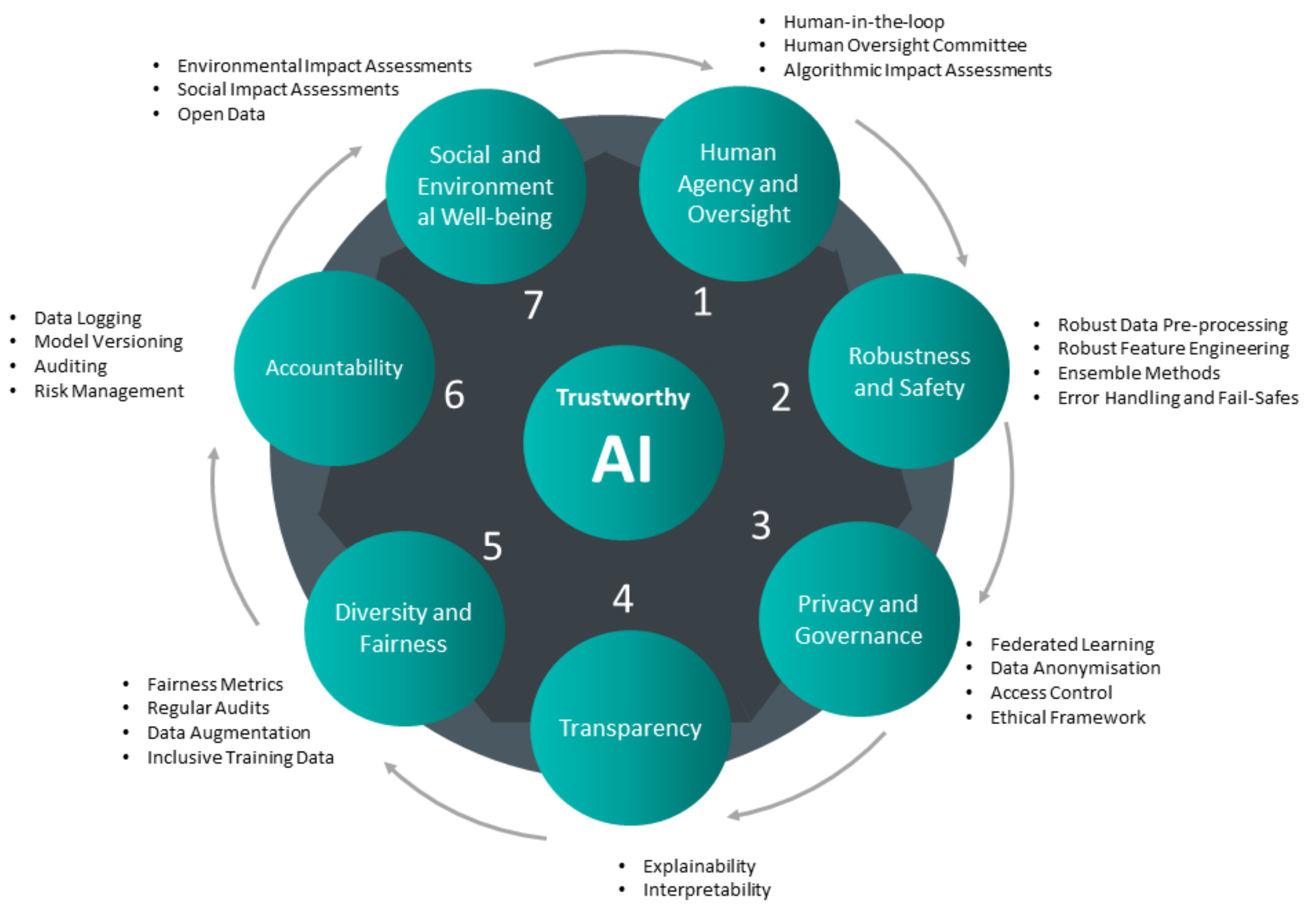
• Human agency and oversight: In order for the AI models to support humans, a proper oversight and supervision mechanism for their performance is necessary. This is attainable by human-in-the-loop concepts.
• Privacy and data governance: This aspect is focused on data protection, integrity, and discretion. It is necessary to be considerate of the requirements and the consequences of illegitimate access to the data.
• Robustness and safety: This is one of the most technical aspects of AI models’ trustworthiness. It is about models and methods to be resilient and robust to reasonable perturbations. Reliability and reproducibility under non-planned scenarios is the main concern of this aspect.
• Transparency: Models and methods integrated with AI algorithms are required to be transparent and traceable. This means they are needed to be more of white boxes than the black boxes of decision-making algorithms. Transparency is necessary to be adapted to each stakeholder’s specific terminology and concerns.
• Fairness and diversity: This is to make sure the algorithms are not biased toward a specific population or group of data. This could lead to discrimination in human-related applications or in poor performance and generalisation in technical applications.
• Social and environmental well-being: While it is expected that all AI systems benefit humans, it is not always clear how this is realised. This aspect is to make sure the implications and advantages on human lives and also on the environment are clarified.
• Accountability: This aspect tries to raise awareness regarding the reproducibility and traceability of the performed works by AI. Performing regular audits and assessments of the algorithms is an important method to make sure they perform well in critical applications.

Having the seven aspects of trustworthy AI (including ML) algorithms makes it worth noting that not all of these items are applicable to (lithium–ion) battery research to equal levels. This is due to the nature of battery data, which are mainly from non-human sources and they are heavily technical. In fact, battery-related data do not face all the challenges that life or social sciences data face. Still, many of the aspects of the EU regulations meaningfully apply to the battery research field. A summary of the example techniques to address these for the battery studies is given in Figure 1.

Addressing the example techniques in Figure 1 is out of the scope of this work and readers are invited to review the relevant resources such as [6,7] for further information.

The particular aspect of transparency indicated in Figure 1 is the main topic of the current paper. ML algorithms are essentially complex with little information available regarding their working mechanism and the flow behind the specific decision or prediction. Although the ML models may not be directly explainable [8], there are solutions that address this missing transparency called explainable or interpretable machine learning (XML/IML). Explainable machine learning is particularly important in the context of lithium-ion batteries, as it allows for a better understanding of the underlying processes and the ability to make informed decisions and predictions. This can be especially useful for identifying and preventing battery failures and for developing control strategies to ensure safety. Explainable ML is more about answering the “WHY” questions when it comes to decision-making or predictions, and this can lead to extra investment in those reasons for quality improvements.

In line with the given motivation, this paper is intended to provide a review of the state-of-art XML and IML techniques for the lithium–ion battery field of research. To the best of the authors’ knowledge, despite the large number of review papers dedicated to various aspects of lithium–ion batteries and ML (such as [3,4,9]), the XML for batteries has not yet been reviewed in any previous works. In summary, this paper will contribute the following:

• A review of the explainability techniques that are been utilised in the battery domain.
• The advantages and challenges of the explainability techniques.
• A categorisation and comparison of the XML methods applied for battery design and manufacturing.
• A review and summary the role of XML in the design and delivery of intelligent battery management systems.
• An identification of the challenges and research gaps in each category.
• A summary of key insights and the future research directions in the area of batteries and XML.

1.1. Materials and Methods

This review has been conducted using several terms in the literature, including lithium–ion battery, battery energy storage, rechargeable battery, machine learning, deep learning (DL), and artificial intelligence. These terms have been combined with the keywords of explainable machine learning, XML, explainable artificial intelligence (XAI), interpretable machine learning, interpretable artificial intelligence (IAI), explainability, interpretability, Shapley, SHAP, dependency, correlation, accumulated local effects (ALEs), partial dependency plot (PDP), feature importance, permutation importance, manufacturing, formulation, design, battery management systems (BMSs), state of health (SoH) estimation, state of charge (SoS) estimation, state of energy (SoE) estimation, and fault detection.

While the battery, lithium–ion, and machine learning key terms individually led to a large number of papers, the combination of those with the explainability, and interpretability and the rest of the above-mentioned keywords narrowed them down to about 100 papers. Among those, the papers that directly included a reference to one of the explainability/interpretability techniques were selected. This selection was managed manually based on not only the title but also the abstract of the papers. This process was followed to filter out the papers that have explainability/explainable terms besides the battery and machine learning keywords, but they only mean generic explanations of the results rather than the application of formal XML/IML techniques.

The particular databases that were searched for papers included IEEEXplore, Science Direct, Nature, MDPI, Wiley Online Library, IOP Science, and Springer. The rest of the papers were hand-picked directly from the Google Scholar web engine. The focus of the search has been on the journal papers, but on some occasions highly cited and credible conference papers were also selected for review purposes. The approach of this paper has been simple search, manual selection, and expert judgment on relevance. The search has included all the papers from all times, up until April 2023. This review assumes that the reader is already familiar with lithium–ion concepts and also has enough background with machine learning techniques.

1.2. Structure of the Paper

This paper has six sections. Section 1 justifies the need and motivation for this review from the battery research community point of view. Section 2 offers the fundamentals, preliminaries, definitions, and main concepts of explainable and interpretable machine learning. The audiences of this section are the researchers with knowledge of ML but less information regarding the explainable and its techniques. This section summarises the key questions raised during the practical use of ML that could be elevated by XML. Section 3 lists and sufficiently explains the key explainability techniques; this is mostly focused on techniques identified to be popular in the lithium–ion research community as well as the methods that heave the potential to be used there. Readers interested in more details on ML and in wider concepts related to AI could refer to the many excellent resources published by the community such as [10,11,12].

Section 4 is focused on the role of XML and IML for the design, manufacturing, and production of battery cells. This section starts with a brief overview of the design and cell manufacturing, and due to the focus of the reviewed articles on lithium-based chemistry, mainly addresses this type of cells. This section and onward have audiences who are expected to be relatively familiar with the challenges of battery design, production, and testing as well as their implementation and usage in real applications. Further details regarding the battery production chain and processes could be found in comprehensive studies such as [13,14].

The aim of Section 5 is to address the applications and impacts of the XML for lithium–ion batteries when in use. It addresses the main battery performance monitoring concepts, including its state of charge, state of health, and state of energy. This is followed by Section 6, which reviews the battery management system aspects combined with XML. Finally, Section 7 summarises the paper and provides discussion, recommendations, and future overviews of this field.

2. Explainable Machine Learning

In this section, the fundamentals, theories, formulae, and definitions of explainable machine learning are addressed to provide a better understanding of its terminologies, variations, and applications.

2.1. Explainable vs. Interpretable ML

In the field of ML concepts, sometimes both words Explainable and Interpretable are mentioned in the literature, and it is usually the case of those being mistakenly considered to have the same meaning. Although explainable machine learning and interpretable machine learning are both closely related and their purpose is to make ML models more transparent, they are different in their specific focus and approach [15].

Interpretability in ML can be defined as the ability to explain a machine learning model by defining it with meaningful terms to a human [15]. Thus, interpretable machine learning focuses on making the model itself more interpretable, typically by using simpler or more transparent model architectures, such as decision trees or linear models. On the other hand, explainable machine learning focuses on providing explanations for the predictions of a machine learning model, regardless of the underlying architecture [16].

In safety-critical applications that include lithium–ion battery design, modelling, and management, it is vital and applicable to include XML for understanding the processes and making informed decisions based on the predictions. Unlike XML, IML may not be applicable to battery research easily. IML is meant to be used to make the model more interpretable and understandable; however, due to the complex nature of the battery-related problems, it is not always possible to have a simple and interpretable model that has an acceptable level of performance or accuracy at the same time. In fact, interpretable but poor is not sufficient to ensure the safety and reliability of the application [17].

2.2. The Need for Explainability

Addressing explainability, the first question that needs to be answered is why explainability is necessary for ML techniques? Generally, the need for XML can be addressed during two main phases of ML techniques, namely (1) their development and then (2) their operation.

During the development phase of ML approaches as solutions, XML is necessary due to the following reasons as described by [18,19,20,21]:

• Data Management—Having XML enables developers to find vague points, missed information, and gaps in our training data.
• Model Selection—XML performs as a criterion for model selection to eliminate the models with vague or non-transparent reasoning from the list of options.
• Model Training—Having an appropriate model selected, XML helps to improve the hyper-parameter optimisation and polishing the model to gain better performance. XML simplifies hyper-parameter tuning, facilitating easy experimentation to find optimal settings. Moreover, XML helps in polishing the model, refining its performance and reliability. Thus, XML is instrumental in streamlining model training, yielding improved performance and more reliable outcomes.
• Model Verification—In model validation and verification, the goal is to define key performance indices and evaluate the trained model. In model verification, XML can be used as a metric to evaluate model behaviour in terms of weaknesses and model flaws as well as finding their main causes.

Similar to the development phase, XML is required for the operation phase [18,19,20,21] for:

• Model monitoring—XML can be used as a diagnostics tool to link back the model results to the data and identify the sources of imperfect behaviour.
• Investigation of accident or incident—Having an issue with the ML on operation, local explainability can help us to understand why the decision is made in the wrong way.
• Run-time improvement—XML can help us to improve the models when new data and different situations are faced.

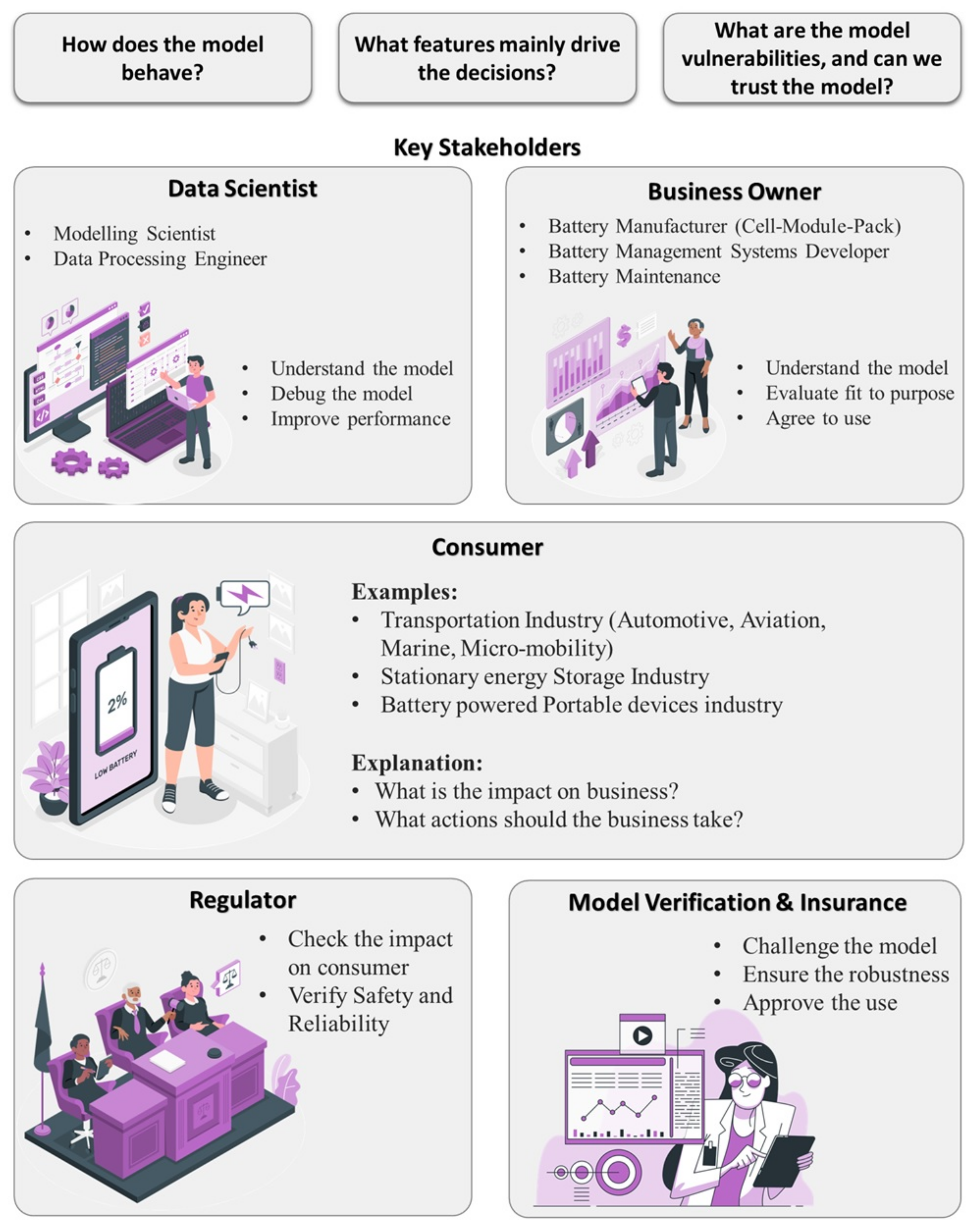
2.3. Role of Explainability among Key Stakeholders

In the lithium–ion battery industry, the development and application of machine learning models is a multi-stakeholder effort. Each stakeholder, whether a data scientist, business owner, regulator, or consumer, has unique perspectives, interests, and requirements, and all play a critical role in the overall success of the model’s deployment. One of the key considerations for all stakeholders is the model’s explainability, or its ability to make its processes and predictions understandable and interpretable to humans. Explainability is essential, as it enables the validation and verification of the model’s results, the correction and improvement of its processes, and the alignment of its functionality with business objectives and regulatory standards. It also allows stakeholders to assess the impact of the model on business, industry, and consumers [22].

Figure 2 provides a structured overview of the key stakeholders involved in the development, evaluation, and application of machine learning models in the context of lithium–ion battery technology. It divides the stakeholders into five categories: Data Scientists, Business Owners, Model Risk Stakeholders, Regulators, and Consumers.

For each category, the figure provides concrete examples of the roles involved. For instance, within the “Data Scientist” category, roles like Modelling Scientist and Data Processing Engineer are listed. Similarly, the “Business Owner” category includes roles such as Battery Manufacturer and Battery Maintenance Professional. The “Model Risk” stakeholder group is represented by insurance companies. Regulators are usually governmental entities while the “Consumer” category encompasses broad industry segments that rely on lithium–ion batteries, like the transportation and stationary energy storage industries.

The figure also details how each stakeholder group may interact with the machine learning model in their work. For instance, data scientists are involved in understanding, debugging, and improving the model. Business owners need to understand the model, evaluate its fitness for purpose, and agree to its use. Model Risk stakeholders are involved in challenging the model and ensuring its robustness. Regulators have the responsibility to verify the model’s impact on consumers and verify safety and reliability, while consumers are interested in understanding the impact of the model on their business and determining necessary actions.

In what follows, major explainability techniques applied to ML models in lithium–ion battery studies, which are listed and summarised.

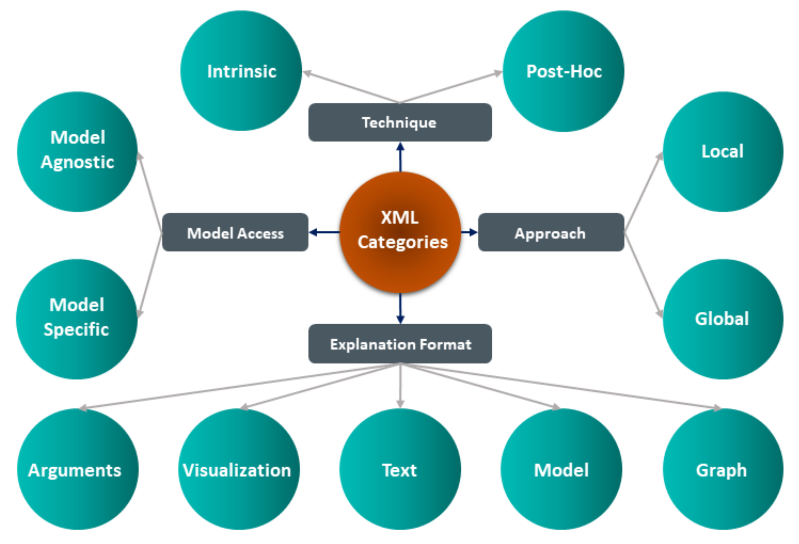
3. XML Categories and Methods

XML approaches, as illustrated in Figure 3, can be broadly categorised into several key dimensions.

Local versus Global: Local explanations aim to clarify the behaviour of a model at a particular instance. In a tabular dataset, this pertains to the explanation of a single row of data. For image datasets, it is about deciphering a specific image’s interpretation. On the other hand, global explanations seek to illustrate the model’s general behaviour across an entire dataset or dataset. An averaged-out explanation from multiple local instances can also give a generalised, global understanding.

Model-specific versus Model-agnostic: Model-specific explanations are tightly tied to the structure of the particular model they are explaining. They take advantage of the unique features of that model for interpretability. On the contrary, model-agnostic explanations can be used regardless of the model’s internal workings, making them broadly applicable across different model types.

Intrinsic versus post hoc: Intrinsic explainability refers to models that are inherently interpretable, meaning the model’s structure and functionality can be easily understood. Post hoc explanations, however, are generated after the model has been trained. They seek to explain a black-box model that may not be intrinsically interpretable.

Explanation Format: This category details the various ways the explainability can be presented. This could be in the form of arguments (logical reasoning behind a decision), visualisations (graphs or charts depicting the model’s functioning), text (written explanations), models (simpler models that can approximate a more complex one), and graphs (networks that represent relationships between elements).

These categories provide diverse perspectives on XML’s applicability in the lithium–ion industry, capturing nuances in explainability, usability, and format preferences.

XML recently has received considerable attention following the newly introduced European General Data Protection Regulation [23], which necessitates accessible justifications for automated decisions. For model developers the explainable means moving from the trial-and-error-based production, [24] and for the users, it means more trust by looking at the rationale behind the decisions and having justifications [25,26].

3.1. Partial Dependence Plot and Accumulated Local Effects

One of the most intuitive and historical approaches to explainability is considering the effects of features on the average predictions, which can be easily visualised considering one or two features (in 2D and 3D). Such approaches reduce the complexity of a prediction function by keeping other features constant and observing the changes in predictions when changing one or two features. Different approaches lie in this category; however, as of this paper, we focus on two more popular approaches that were addressed in the reviewed papers, namely Partial Dependence Plots and Accumulated Local Effects.

Partial Dependence Plots (PDPs or PD Plots) [27] show the marginal effect of one or two features on the outcome of the predictive model to better describe the relationship between the target and these features. PD Plots work based on marginal distributions. For a regression task, the partial dependence function is defined as Equation (1) [28]

$${\widehat{f}}_S\left(x_S\right)=E_{X_C}\left[\widehat{f}(x_S,X_C)\right]=\int \widehat{f}(x_S,X_C)d\mathbb{P}\left(X_C\right)$$

(1)

In the above equation, the machine learning model is denoted with $\widehat{f}$, $x_S$ refers to the features that PDPs represent, and $X_C$ are other remaining features. S refers to the feature set (which includes a maximum of two features as discussed earlier) that PDPs are depicted for and represents their effects on the predictions.

Although this approach is very intuitive, it suffers from some issues: correlated features, heterogenous effects, and extrapolations. Hence, in reality, these plots alone are not sufficient for addressing interactions among the features. In the face of correlated variables, where a change in one variable also changes the other, it is not always straightforward to infer whether the change in the response is due to the change in a specific variable or if it could be because the other correlated variable is also changing. Another pitfall of PDPs is having heterogeneous features where their effect cancels out each other on average; this may be misleading and interpreted as not having any effect on predictions. Additionally, PDPs do not work well when out-of-distribution data are fed to the model (extrapolation). To address some of the mentioned challenges, the Accumulated Local Effects offer a solution.

The ALE [29] plot is a way to analyse the average influence of features on the predictions made by a machine learning model. This technique is faster and unbiased in comparison to Partial Dependence Plots.

To compute the ALEs for a specific feature, the feature space is divided into intervals, denoted as $N_j\left(k\right)$. The number of intervals is determined by the machine learning expert based on numerous considerations, such as computational complexity and data limits. For data within each interval, the ALE is calculated by taking the difference between the predictions made by the model $\tilde{f}$ when the feature value is replaced with the upper and lower limits of that interval. These differences are then accumulated and averaged as formulated by Equation (3) [28]:

$${\widehat{\tilde{f}}}_{j,ALE}\left(x\right)={\displaystyle \sum _{k=1}^{k_j\left(x\right)}}\frac{1}{n_j\left(k\right)}{\displaystyle \sum _{i:x_j^{\left(i\right)}\in N_j\left(k\right)}}\left[\widehat{f}(z_{k,j},x_{-j}^{\left(i\right)})-\widehat{f}(z_{k-1,j},x_{-j}^{\left(i\right)})\right]$$

(2)

In the above equation, $\widehat{f}$ represents the machine learning model. $N_j\left(k\right)$ refers to the neighborhood defined by the intervals. z or grid values are replaced with the features of interest. Also, $n_j\left(k\right)$ represents the number of instances in this interval. The ALE obtained from Equation (2) is then centered as follows (Equation (3)) to ensure a mean effect of zero [28].

$${\widehat{f}}_{j,ALE}\left(x\right)={\widehat{\tilde{f}}}_{j,ALE}\left(x\right)-\frac{1}{n}{\displaystyle \sum _{i=1}^n}{\widehat{\tilde{f}}}_{j,ALE}\left(x_j^{\left(i\right)}\right)$$

(3)

By doing so, as the name suggests, “local” areas are defined for the features. Then, within each local area, data samples that fall within the area are selected within the designated ranges. Then, the values are changed while other features are kept fixed across the samples. Finally, the prediction difference is calculated from the start to the end of this area. This process is repeated for all defined areas and then, by accumulating these local effects, the overall influence of the input on the output is determined.

In summary, both ALE and PDP approaches describe the influence of features on the average predictions. The main difference between these two approaches is that PDP considers the average predictions for a specific value while ALE calculates the difference between predictions in a small window around the specific value. Furthermore, PDP is performed over marginal distribution while ALE is based on the conditional distribution of features. ALE is faster and more reliable as it is not biased when having correlated features. Additionally, ALE is easier to interpret as the relative conditional effect is visualised as opposed to PDP which depicts the average prediction. To overcome the PDP and ALE challenges, a fairly newer approach called Differential Accumulated Local Effects (DALEs) is introduced. DALEs being out of the scope of this paper can be followed in [30].

3.2. Feature Importance

This subsection explores various methods to ascertain the significance of features within a model. The Permutation Feature Importance technique shuffles a feature’s values to measure the resulting decrease in model performance. The Gini Importance method, applied to tree-based models, considers the total decrease in node impurity. LASSO employs variable selection and regularisation to identify important features. Saabas calculates feature importance based on average prediction change from feature splits across all trees. The Gain method measures the reduction in the loss function by all splits over a feature, and Split Count quantifies the frequency a feature splits data across trees.

3.2.1. Permutation Feature Importance

This method involves shuffling the values of a feature and measuring the decrease in the model’s performance. The idea is that an important feature, when shuffled, will drastically reduce the model’s performance. The permutation feature importance of a feature i is defined as [31,32]

$$PI\left(i\right)=\frac{1}{n}{\displaystyle \sum _{j=1}^n}[L(y,f\left(X\right))-L(y,f\left(X^{(i,j)}\right))]$$

(4)

where $PI\left(i\right)$ is the permutation importance value, the n is the number of permutations, L is the loss function, y is the true output, $f\left(X\right)$ is the model’s prediction with the original dataset, and $f\left(X^{(i,j)}\right)$ is the model’s prediction with the j-th permutation of feature i [11]. There are different variations for permutation-based feature importance that can be found in the literature [33,34,35,36,37].

3.2.2. Gini Importance

This method also known as Mean Decrease impurity is often used in tree-based models. The Gini Importance of a feature is calculated as the total decrease in node impurity, weighted by the probability of reaching that node, averaged over all trees in the ensemble [38]. The Gini Importance of a feature i can be formally defined as

$$GI\left(i\right)=\frac{1}{T}{\displaystyle \sum _{t=1}^T}{\displaystyle \sum _{j\in N_t\left(i\right)}}p\left(j\right)\Delta Gini\left(j\right)$$

(5)

where T is the total number of trees, $N_t\left(i\right)$ is the set of nodes j in tree t that split on feature i, $p\left(j\right)$ is the proportion of samples that reach node j, and $\Delta Gini\left(j\right)$ is the decrease in Gini Impurity due to the split at node j [39].

3.2.3. LASSO

LASSO (Least Absolute Shrinkage and Selection Operator) is a regression analysis method that performs both variable selection and regularisation. The features with non-zero coefficients are considered important. The LASSO optimisation problem can be defined as [40,41]

$$\underset{\beta }{min}\frac{1}{2n}\left|\right|y-{X\beta \left|\right|}_2^2+{\lambda \left|\right|\beta \left|\right|}_1$$

(6)

where y is the output vector, X is the input matrix, $\beta$ is the coefficient vector, n is the number of samples, and $\lambda$ is the regularisation parameter.

3.2.4. Saabas

Saabas, introduced by Ando Saabas in [42], is an individualised heuristic feature attribution method that is often used with tree-based models. It computes feature importance by considering the average change in the prediction caused by a split over a feature, averaged over all trees. Unlike the previous methods based on performance loss, Saabas measures the change in the model’s expected output directly for comparisons. The Saabas importance of a feature i can be defined as Equation (7), fully traceable in [42,43].

$$Saabas\left(i\right)=\frac{1}{T}{\displaystyle \sum _{t=1}^T}\sum _{j\in N_t\left(i\right)}p\left(j\right)\Delta pred\left(j\right)$$

(7)

Here, T is the total number of trees, $N_t\left(i\right)$ is the set of nodes j in tree t that split on feature i, $p\left(j\right)$ is the proportion of samples that reach node j, and $\Delta pred\left(j\right)$ is the change in the prediction due to the split at node j.

3.2.5. Gain

The Gain method, introduced by Breiman et al. in 1984 [39], quantifies feature importance based on the total reduction in the loss function or impurity achieved by all splits over a given feature. Despite its heuristic nature [44], Gain is widely adopted for feature selection [45,46,47]. The Gain importance of a feature i is described by Equation (8),

$$Gain\left(i\right)=\frac{1}{T}{\displaystyle \sum _{t=1}^T}\sum _{j\in N_t\left(i\right)}\Delta Loss\left(j\right)$$

(8)

where T is the total number of trees, $N_t\left(i\right)$ is the set of nodes j in tree t that split on feature i, and $\Delta Loss\left(j\right)$ is the decrease in the loss or impurity due to the split at node j. This measure offers a comprehensive view of a feature’s contribution to the model.

3.2.6. Split Count

Split count is a measure of the number of times a feature is used to split the data across all trees. The Split Count importance of a feature i can be defined as [48]

$$SplitCount\left(i\right)=\frac{1}{T}{\displaystyle \sum _{t=1}^T}\left|N_t\left(i\right)\right|$$

(9)

where T is the total number of trees and $N_t\left(i\right)$ is the set of nodes j in tree t that split on feature i. This represents both the closely related “weight” and “cover” methods in XGBoost, but is computed using the “weight” method.

3.3. SHAP

SHapley Additive exPlanations (SHAPs) indicate how each feature is contributing to the overall prediction of the response variables. SHAP assigns each feature an importance value for a particular prediction [49]. The SHAP framework includes Tree SHAP for decision tree-based models, Kernel SHAP for kernel-based models, and Deep SHAP for deep learning models. Each variant has its unique strengths and weaknesses, and the choice should be guided by the model architecture and the data characteristics.

SHAP values are calculated based on Shapley values from cooperative game theory. Each feature’s contribution to the prediction is fairly attributed, considering all possible combinations of features. The SHAP value for a feature i in a model f is given by

$${\varphi }_i\left(f\right)=\sum _{S\subseteq N\setminus i}\frac{\left|S\right|!\left(\right|N|-|S|-1)!}{\left|N\right|!}[f(S\cup i)-f\left(S\right)]$$

(10)

where N is the set of all features, and S is a subset of N that does not include feature i. This equation sums over all possible subsets of features, attributing the difference in the model’s output with and without feature i to the SHAP value of feature i.

One of the unique advantages of the SHAP is the offer of visualised dependencies such as dependence plots, and force plots for model interpretability [50] that allow users to understand the contribution of each feature to the model prediction.

3.4. Pearson Correlation

SHAP not only is used for contribution analysis but is also a way to quantify the correlations between the input and responses. A more traditional way of correlation analysis is also Pearson correlation, which quantifies the linear relationship between two datasets [51] and can be described as (11)

$$r=\frac{{\displaystyle {\sum }_{i=1}^n}(x_i-\overline{x})(y_i-\overline{y})}{\sqrt{{\displaystyle {\sum }_{i=1}^n}{(x_i-\overline{x})}^2{\displaystyle {\sum }_{i=1}^n}{(y_i-\overline{y})}^2}}$$

(11)

where r is the Pearson correlation coefficient, n represents the number of data points, $x_i$ and $y_i$ are the individual data points for the two variables in consideration, $\overline{x}$ and $\overline{y}$ denote the means of the x and y datasets, respectively.

Compared to SHAP, Pearson is less advantageous when dealing with correlated input variables in relation to the responses, and is not able to deal with categorical features either.

3.5. Explainability Considerations

Having the main techniques of XML reviewed in the previous section will full detail, this subsection is dedicated to the common and still existing challenges of XML in real applications including the lithium–ion battery field of research.

3.5.1. Data Importance

According to research, even capturing data points from a mere 18 experiments in battery cell manufacturing can take up to six months in a pilot-line manufacturing assembly [52]. These experiments can involve various stages of testing and trials, each generating its own unique data which must be processed and interpreted. The slow accumulation of relevant data can significantly delay advancements in battery technologies and their subsequent implementation into marketable products.

Given these challenges, the concepts of data importance and data valuation are particularly pertinent to machine learning and explainability in the lithium–ion industry. Essentially, the goal is to determine which data are most valuable and crucial to the modelling activities and to prioritise the collection and analysis of these data. Data Shapley is a method in which the importance of each data instance is evaluated using the Shapley value from cooperative game theory, within the context of supervised learning [53]. By this method, through attributing a Shapley value to each data point, a measure of data importance that considers both the individual contribution of a data point and its interaction with other data points in the dataset is obtained.

3.5.2. Counterfactual Explanations

Counterfactual explanations, distinct from other forms of explainability, extend the understanding of Machine Learning/Deep Learning (ML/DL) models beyond the “why?” to include hypothetical scenarios, often phrased as “what if?” queries [28,54]. These explanations enable us to delve deeper into an alternative reality wherein input variables could take on different values, helping to elucidate potential changes in model predictions. In any application, including the lithium–ion battery industry, these explanations provide insights into cause-and-effect relationships between input variables and predictions [55].

Considering the lithium–ion battery industry, counterfactual explainability can help ML designers to predict the effect of each variable on the prediction as well as the points for which the variable can toggle the predictions.Counterfactual explanations allow ML designers to answer questions such as “What would have happened if a certain input variable had a different value?” or “For a classification task, how a change in a certain input variable can change the prediction to the other class?” [22,56,57,58].

This information can be used to create a better picture of ML/DL behaviour as well as identification of areas for improvement in the battery design and to optimise battery performance based on its ML/DL model [59,60,61].

For instance, if an ML model predicts high capacity for a specific battery configuration, counterfactual explanations can guide engineers to discern why this is the case, thus enabling them to devise modifications to the design to further enhance capacity [62]. Hence, counterfactual explanations offer additional layers of understanding, allowing practitioners to explore potential outcomes and improvements beyond the immediate model predictions.

3.5.3. Explainability Weaknesses

The idea behind the explainability is to provide a clear explanation of the model behaviour, and this is a vital step towards trustworthy machine learning algorithms implementation. However, there are some cases in which even XML techniques fail to provide a correct explanation for the models’ behaviour. As an example, [63] has focused on deep neural networks and their explainability using gradient-based methods. The author depicted a case in which the input sample is close to the decision boundary and shows how a small change in its value can make the gradient-based explainability incorrect. In another case, Slack D. et al. [64] have used adversarial attacks on post hoc explainability methods such as SHAP and have illustrated examples in which they failed to provide a correct explanation. For instance, for a tabular dataset, it has created an unrelated feature, and with an adversarial attack, the explainer is shown to be fooled. Another example is dedicated to pushing the explainer and making it biased towards a particular feature to show that this could be a common case in many datasets.

Wrapping up the XML techniques in this section, the upcoming sections are focused on the application and the role of XML in lithium–ion battery technology. Based on the review, almost all of the references follow a similar pipeline for modelling and explanation which is summarised in Figure 4. The sections while separated during the various phases of the technology development, production, and implementation within an application, all follow the order of problem definition, the modelling technology, the explainability methodology, and finally the results and conclusions from that.

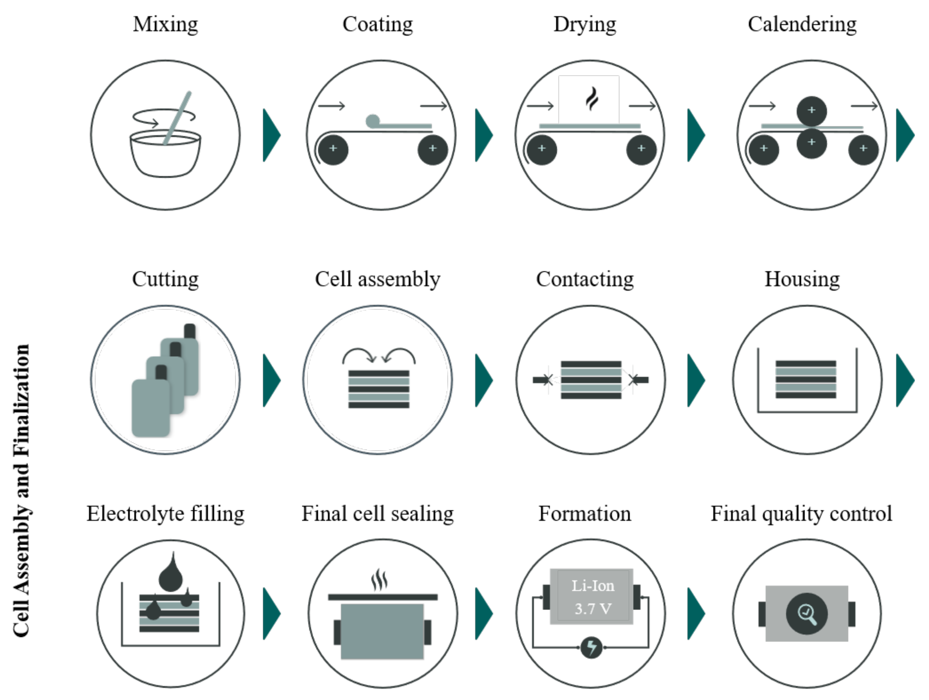
4. XML in LiB Electrode Manufacturing and Cell Production

In recent years, artificial intelligence has found its way into the optimisation, control, and analysis of lithium–ion battery cell production. The LiB cell production is a long and consecutive process chain consisting of three main phases: electrode manufacturing, cell assembly, and cell finalisation. The slurry’s formulation is an additional aspect that can be considered as part of the battery cell production, which has been investigated in recent years. Figure 5 provides an overview of the common process steps along the LiB production chain. The details of the production processes can be found in [65,66].

When it comes to the LiB process control and optimisation, there is a large number of control and response variables that need to be analysed and addressed appropriately. This large number of control variables, as well as the equipment settings, pose a major challenge when it comes to optimising them for a desired characteristic of LiBs. Also, the complexity and the multi-physics-based nature of the individual processes, as well as the interaction between one process and another, add to the difficulty of developing analytical, numerical, or finite element models which can be universally applicable across a broad spectrum of control variables and desired responses. The nature of this problem makes the AI and ML models very well suited for modelling the inter-dependencies between the control and response variables in battery cell production. The following subsections provide an overview of the existing research on battery cell production that benefit XML.

4.1. Formulation and Mixing

The physical and electrochemical characteristics of LiBs heavily rely on the combination of materials in their components, including positive and negative electrodes. Understanding the impact of the various materials and their ratios, the formulation is the key to optimising cell performance. Such optimisation is often very challenging to be handled due to a large number of inter-connected factors. ML techniques based on carefully designed experiments could offer a solution and when enhanced by explainable techniques could be taken one step forward to realisation in scale manufacturing.

In this context, a recent XML study on a particular class of batteries with doped lithium nickel–cobalt–manganese cathodes has adopted SHAP to understand the governing dopant feature of the electrode on the discharge capacity of cell’s material [67]. The study develops six machine learning models of Gradient Boosted Trees (GBT), Random Forest (RF), SVM, K-Nearest Neighbour (KNN), ANN, and kernel ridge regression (KRR), to investigate the correlation between the structural characteristics identified by domain expert related to 168 cells with their discharge capacity during the first and 50th cycle. Among all models, the GBT provides the best prediction accuracy. The feature importance and feature correlation were analysed through Shapley values, which were believed to be more desirable than the permutation-based analysis. Shapley values were calculated for the best-performing model on the test data for each response variable and the calculations were performed via TreeSHAP. Based on the feature importance analysis, the minimum and maximum cut-off voltage, as well as the current density, were identified as the most significant factors determining the discharging performance of the material as a cathode at the cell’s initial and 50th cycle. These features were followed by the dopant content and the lithium content ratios. The Shapley values here also have shown that, with higher contents of lithium, smaller amounts of dopant, and atoms with lower electro-negativity, the cells become more likely to have a higher first and 50th cycle discharge capacity.

Liu et al. in [68] has analysed the impact of formulation on the electrode thickness, electronic conductivity, and half-cell capacity, specifically for LFP and LTO chemistry. The study is based on the dataset published in [69], which consists of 138 data points for LFP and 108 for LTO electrodes. The existing data were divided into three categories for classification and exhibited a significant class imbalance. In order to address this imbalance issue of the data, [68] proposed a framework based on Random Under-sampling Boosting (RUBoost). Here, for the case of explainability, the relevance of the parameters was analysed using the Gini index and linear correlation. For both thickness and capacity, all the formulation variables except the binder type were identified as relevant with high Gini importance values. For the case of electronic conductivity, the carbon conductive additive (C65) showed the highest impact, followed by the amount of active material. To validate the outcomes of the proposed framework, four additional tree-based models were employed and compared to the developed RUBoost model. The proposed approach showed the best performance in comparison with the other developed models with an F1-score of above 80% for both LFP and LTO electrode thickness.

For a commercial LiB cell chemistry, a cathode to anode ration study via XML is reported in [70]. Here, the researchers have investigated the impact of the ratio between the negative and positive electrode capacity (N:P ratio) during cell manufacturing on the final cell’s characteristics in terms of its energy capacity. The study is based on input factors determined by domain experts and the data related to 48 cells with the control factors of N:P ratio cathode and anode areal capacity, cathode and anode active material weight, and their thicknesses. Based on the data obtained via a design of experiment, a random forest model has been developed and validated via a five–fold cross-validation approach. The models show an acceptable level of accuracy, which is an R2 of 0.905 for capacity at low crate of C/20, 0.779 for capacity at high crate of 5C, and 0.885 for the capacity ratio (5C to C/5). The study includes the explainability of the models via methods of SHAP average values for feature importance analysis and ALEs.The feature importance analysis showed that the cathode active material and its thickness are the most important features for the cell capacity up to 5C, while the anode active material also plays a pretty important role in the 5C capacity of cells. At all crate values, the N:P ratio is the relatively least important factor compared to the other inputs, which revealed that, for a comprehensive study, a well-designed experiment is required, ensuring that the N:P ratio is not overshadowed or masked by other features. The ALEs also highlighted the nature of dependency between N:P ratio and cell capacity, which was shown to be linear and inverse for C/20, including a local maximum for the 5C capacity.

In a comprehensive analysis, [71] investigates the impact of slurry mixing and coating variables on the physical characteristics of the electrodes and the quality of the half coin-cells. The adopted algorithms are RF and GBTs in the configuration of Figure 6 with nine control factors related to six response variables selected by the domain expert.

This study shows that, while the model is able to predict the responses with $R^2$ values between 0.746 for coating density and 0.942 for wet thickness of the electrode, the explainability methods of ALEs and feature importance can successfully describe the relations between the input and output variables. The feature importance analysis based on the mean decrease in impurity index [72,73] has been carried out and revealed that the coating gap is the dominant feature at all responses with a considerable share on the predicted response. It massively masks the impact of other factors, especially for the thickness of the coating and the cell capacity. Based on this explanation, the authors have suggested a revised design of experiments and a new study to be carried out after removing this factor, so the impact of other features becomes more vivid. This study is almost the first that has managed to quantify the impact of features on the responses and explain the trend of variables via first- and second-order ALEs. It has been shown that, while the coating gap contributes linearly and directly to coat weight, the viscosity has a direct but saturated impact curve.

4.2. Coating and Calendaring

In data-driven studies dedicated to electrode manufacturing, the coating process stands out as one of the most extensively analysed process steps [9]. Several studies have utilised different methods, such as feature importance and feature ranking or SHAP to increase the interpretability of the developed coating process models. In the following section, a brief review of these studies is provided.

Benefiting from the dataset in [74], the authors of [75] have adopted RF to classify the mass loading and porosity of electrodes as two important intermediate product properties during manufacturing. For this purpose, the mass content of active material, the solid-to-liquid ratio of slurry, viscosity, as well as the comma gap during the coating process, are considered as input variables. The dataset consists of 656 samples in total for 82 configurations, where five classes were defined based on both mass loading and porosity levels as output variables. The significance of input variables was quantified using feature importance, particularly the unbiased FI and gain improvement-based techniques. In the case of mass loading classification, despite the notable discrepancies in the results obtained from the two adopted methods, the overall trends were observed to be similar. The comma gap was identified as the most significant variable via XML analysis, while the viscosity of the slurry demonstrated the least contribution to the classification results. Using a similar approach, the significance of the input variables in combination with the electrode porosity was analysed. As a result, the solid-to-liquid ratio of slurry and its viscosity were identified as the most contributing features, with the mass content of active material being the least important feature. Based on the obtained insights, the performance of the developed models was evaluated using different sets of features. While the results could confirm the feature importance evaluation, a relatively poor performance was reported for the model classifying porosity, suggesting that additional quality-relevant parameters should be considered in the dataset.

The same data available by [74] were once again incorporated into a Gaussian Process Regression (GPR) framework for continuous prediction of the electrodes’ mass loading in Ref. [76]. The study investigates different Automatic Relevance Determination (ARD) kernel structures of GPR to determine the weights of individual features and assess their influence on the prediction of mass loading. Across the four different kernel structures, almost the same trends were observed for the feature with different weights. The comma gap feature was demonstrated to have the highest impact, while viscosity was exhibited to have the lowest influence on the prediction of mass loading. Among the four ARD kernel functions, the ARDMatern5/2 exhibited the best performance in predicting mass loading, with a root mean square error (RMSE) of 1.204 mg/cm². Among the four different models, the ARDEX kernel-based model stands out with the shortest training time; however, the model exhibits the poorest performance in terms of RMSE, with a value of 1.177 mg/cm². Coating gap has been identified as the most important feature to predict mass loading, while the viscosity has the least contribution in all four different models.

Keeping the focus on mass loading and porosity as major electrode properties, [77] has adopted tree-boosting-based models for the dataset of [74]. In this case, to evaluate the importance of each input variable, the Gini index, as a measure of impurity, was adopted. Additionally, the Predictive Measure of Association (PMOA) was used to carry out a correlation analysis. The developed models were evaluated using a five-fold cross-validation. The sensitivity analysis results for both porosity and mass loading were in line with the findings from the previous study, [75]. In the case of mass loading, the coating gap demonstrates the highest Gini index, while the viscosity has the lowest value. Concerning the electrode porosity, the viscosity along with the solid-to-liquid ratio has been identified as the most influential feature. Furthermore, the study included a comparison of the developed RF models with three other common classification algorithms, including decision tree, k-NN, and SVM. The RF has shown the best performance, followed by SVM for both mass loading and porosity.

To address both cathode and anode, unlike many of the previously mentioned works that only focus on the cathode, [78] has conducted a systematic design of experiments to explore the predictability of properties. Following a correlation analysis, the comma bar gap, web speed, and coating ratio were identified as relevant input parameters to be considered in the modelling for the cathode. In the case of the anode, only the comma bar gap and the coating ratio were determined. The final dataset included 32 configurations for the cathode and 25 configurations for the anode. In the first step, the input variables from the coating process were used to predict the electrode characteristics, particularly the mass loading and electrode thickness. Additionally, the capacity of the half-cell at C/20 was considered as an output variable. The inter-dependencies were modeled using GBT and RF algorithms. The relevance and contribution of each feature were quantified using Mean Decrease in Impurity (MDI) and SHAP values to increase the explainability. Among the analysed output variables, mass loading has been highlighted as the one with the highest accuracy. In general, the GBT models exhibited slightly better performance than RF, regardless of the output variables. Compared to the cathode, the predictability of anode mass loading, thickness, and capacity was slightly lower. Here, the feature importance analysis revealed that, among the input parameters, the comma bar gap and the coating ratio are the primary factors influencing both the mass loading and thickness, with the comma bar gap having the greatest impact. The same trend was observed for the cell capacity.

The inter-dependencies between product parameters in the coating process and the resulting cell capacity have been investigated in a comprehensive study by [79]. A similar study is conduced by [80,81] with neural networks, SVMs, and GBTs boosted with feature importance analysis of the data reported in [79]. The study primarily focused on the cathode; hence, a half-cell coin format was used for the cell characteristics. With the mass loading, electrode thickness, and porosity defined as input variables, an RF-based regression model was developed using the data from 115 coin cells. The cell capacity, as well as gravimetric and volumetric capacity, were defined as output variables. To gain insights into the dynamic impact of variations in the analysed coating parameters on battery capacities, the authors employed the ALE explanation methodology. This included the analysis of single features as well as feature pairs such as mass loading and thickness. Among the analysed coating parameters, it was observed that the electrode thickness had the greatest impact on the cell capacity, followed by the mass loading. In the case of the gravimetric capacity, the mass loading had the highest interaction value. The electrode thickness was identified as the primary contributing factor to the volumetric capacity. The study included the importance ranking of the analysed coating parameters using the aggregated Gini index. The main trends observed in the ALE analysis were also confirmed using the Gini index.

Addressing the calendering process of electrode manufacturing, in [82] the authors proposed a hybrid framework to combine experimental data with in silicomodels, calculating the electrode mesoscale properties. The models are boosted with ML algorithms to analyse the inter-dependencies. The experimental data consisted of the active material content, the electrode thickness before calendering, and the calendering pressure. The electrode mesoscale properties included the tortuosity and the electrolyte effective conductivity. The Sure Independent Screening and Sparsifying Operator (SISSO) was chosen as the ML algorithm. The Pearson Correlation analysis, [51], was also used to demonstrate the impact of different features. For instance, the calendering pressure, compared to the initial electrode thickness, has been shown to have a higher impact on the electrode tortuosity. The results emphasise that achieving optimisation in the manufacturing process is heavily dependent on a complex interplay of trade-offs.

In another calendaring process study, ref. [52] has investigated the impact of process parameters, machine settings, and a combination of electrode properties on the cell’s characteristics. The input variables included the roll temperature, the calendering gap, the mass loading of the electrode, and the target porosity. The dataset comprised a total of 18 different configurations. For the electrochemical characterisation of the produced electrodes, the impedance and the stress test for half cells with 50 cycles were adopted. For the modelling, the Extra Trees as an extremely randomised decision tree model was used in combination with XAI methods such as SHAP and ALE. Regarding capacity, the model exhibited strong performance, with $R^2$ values consistently exceeding 0.95. However, the performance tended to diminish at higher cycles with an $R^2$ of 0.75 at 50 cycles. The model predicting the impedance achieved an average $R^2$ value ranging from 0.75 to 0.85, indicating reasonably good predictive performance. Via XML, the electrode density and porosity were identified as the key features with the highest SHAP value to predict the impedance, while the mass loading and the thickness were highlighted as major features to predict the cell capacity.

4.3. Cell Assembly and Finalisation

In a holistic explainable analysis, ref. [83] has presented a data-driven approach to investigate and improve battery cell production. The proposed approach includes an overview of relevant data sources and possible acquisition strategies. A case study for the application of data-driven models in battery cell production is presented, which is based on the data collected from a pilot line. The dataset includes 772 intermediate product features in combination with the cell characteristics of 167 pouch cells. Due to the high number of features compared to the available data points, only 15 features have been picked to be used in the model development. DT and RF were adopted to model the inter-dependencies between the selected features and the maximum cell capacity. $R^2$ values of 0.723 and 0.748 were reported for the developed models. The study includes normalised feature importance values for features selected from dispersing, calendering, cell assembly, and laser cutting processes. The most important features were reported to be the yield point and the mass of the battery cell prior to electrolyte filling.

Based on the proposed approach in a similar study to the previous one, ref. [84] has presented a use case for predicting the cell capacity using RF and ANN. Using a five-fold cross-validation, all the developed models exhibited a predictive performance with $R^2$ values ranging from approximately 0.66 to 0.79, with the linear Lasso–Lars regression showing the best performance. The study includes the features’ importance for the developed regression model.

Table 1. Overview of the articles using XML methods in battery cell production and the analysed process steps.

Publication	Ref.	Formulation	Mixing	Coating	Drying	Calendering	Cutting	Cell Assembly
Duquesnoy et al., 2020	[82]	x				x
Faraji Niri et al., 2022	[52]					x
Faraji Niri et al., 2022	[78]			x
Faraji Niri et al., 2022	[70]	x		x
Faraji Niri et al., 2022	[71]	x	x
Liu et al., 2021	[76]	x		x
Liu et al., 2021	[75]	x		x
Liu et al., 2022	[77]	x		x
Liu et al., 2022	[79]			x
Liu et al., 2022	[68]	x
Turetskyy et al., 2020	[84]		x	x		x	x	x
Turetskyy et al., 2020	[83]		x			x	x	x
Wang et al., 2021	[67]	x

summarises the reviewed articles in battery cell production and the aspects analysed and reported in those.

5. Application of XML in Battery Modelling and State Estimation

Regardless of the application, ensuring the battery’s long life, desirable performance, and safety is necessary during its charge, discharge, and even when not in use. For this purpose, an accurate estimation of the battery’s internal states is critical but challenging. This challenge is due to the complex interconnection between the cell’s internal and external variables that affect its behaviour. In this concept, three main variables that require to be accurately estimated via affordable techniques are its state of charge (SoC), state of health (SoH), or what is called the remaining useful life (RUL) and state of energy (SoE). There exist various methods for state estimation of batteries, starting from experimental approaches for direct measurement, [85], such as open circuit voltage measurement, terminal voltage measurement, impedance-based and impedance spectroscopy methods, to the simple calculation methods such as Coulomb counting for SoC, to the full benefit of model-based methods such as Kalman filters [86], AI techniques including a variety of ML models and DL prediction [87], as well as fuzzy logics [88].

In this section, first a brief definition and overview of the battery state variables is given; then, the role, application, and benefits of XML for their estimation are summarised.

5.1. State of Health Estimation

Lithium–ion batteries in any application face a capacity loss over time. Even when the cells are not in use, they exhibit a degradation which is called calendar aging [89]. It has been verified that this capacity loss could be due to a variety of failure mechanisms such as a reduction in electrodes porosity [90], growth in the solid electrolyte interface [91], or active material particle cracks [92].

The state of health for a cell is usually defined as the ratio of its available capacity to the initial capacity at the start of the usage [93]. In some occasions, it could also be defined as the battery’s internal resistance in relation to its initial resistance [94]. The threshold after which the battery is considered at its end of life (EoL) depends on the application; in the automotive industry this threshold is usually 80% [95]. Accurate estimation of the battery health status is critical in order to guarantee a safe usage of cells, determining the right time to end their life, or transferring and reusing them for a second life application. This concept is usually referred to as the state of health or remaining useful life estimation.

According to the literature review process followed by authors for battery health estimation, it was observed that the studies related to battery health estimation are mainly using either SHAP or feature importance as their explainability measures. Therefore, in what follows the works are reviewed starting from SHAP and versions, to the feature importance and correlation analysis.

Table 2. Summary of the studies with XML for SoH/life estimation.

Publication	Ref.	Correlation	Feature Importance	Dependency
Lee et al., 2022	[96]	x
		SHAP
Mawonou et al., 2021	[97]		x
Jiang et al., 2021	[98]	x
		SHAP
Li et al., 2023	[99]	x	x
		SHAP
Granado et al., 2022	[100]	x
		Pearson
Zhang et al., 2022	[101]		x	x
				PDP
He et al., 2022	[102]		x
Ibraheem et al., 2023	[103]	x	x
		Pearson
Ardeshiri & Ma, 2021	[104]	x	x
		Pearson
Kim et al., 2022	[105]		x
Wang et al., 2023	[106]		x
Rieger et al., 2023	[107]		x

summarises the list of papers with explainability addressed in there which are covered in this section.

In the context of XML for SoH estimation, one of the distinctive studies is [96], which proposes an estimation method for 379 LiBs at their early phase of qualification tests at a constant temperature. This study addresses one of the largest datasets in the field where the tests were designed for accelerated aging by stress for 5 months. This is mentioned to be equal to 2–4 years of normal use conditions. The method uses a moving window approach for extracting the features of the cell capacity fade curves over 900 cycles. The extracted features include moving averages, moving first-order differences, and moving variances. Here, the features are used for training and validating a variety of machine learning models such as random forest, gradient boosted trees, support vector machines, and Multi-Layer Perceptron (MLP) models. The models have been evaluated based on different lengths of cycles such as 100, 150, to 250 for a target of predicting the next 300 to 700 cycles. The mean absolute percentage error for models is shown to be variable between 0.88% for RF with 150 cycles of training and then a prediction for 300 cycles, it goes up to 13.16% for MLP for 100 initial cycles and an estimation of the 700 cycles. For explaining the ML models, the SHAP is used here. SHAP values are calculated in relation to the three above-mentioned features for the different lengths of training data of the RF model. To reduce the computational cost, the TreeSHAP version is preferred [108]. The local level (a specific target of prediction) and global level (across all experimental conditions) SHAP values have shown that the contribution of the statistical features is very different from one scenario to another. The global analysis has revealed that estimated values of SoH are higher for smaller values of first-order difference features across the moving window, while the predictions are smaller than average for a larger moving average value. The SHAP related to the moving average in relative comparison to the first-order difference values shows that the change in SoH is much more important for the model than the SoH value itself. This explanation is also confirmed via the average SHAP across every 10 cycles for all features. It also shows that the features of the cycles between 60 and 100 are the most contributing ones to the SoH estimation at cycle 700. Such analysis successfully quantifies the importance of early life tests on the estimation of life at a later cycle.

Almost the same objectives and approaches reported by [96] have also been given in [99] but instead use a stacking ensemble model for estimating the cell SoH via Shapley values and feature importance metrics. The dataset here includes 300 voltage profiles from which aging features are extracted via predefined lengths of windows from the battery voltage profile. The study calls them the short-term aging profile and addresses those via the variance, root mean squared values, skewness, kurt value, and the variance of the short-term profile differences. The stacking ensemble model here is trained via five base models of light gradient boosted trees, the random forest, support vector regressors (SVR), XGboost, and the GPR. It is shown that the stacking model has only an RMSE of 1.489% compared to that of 1.751 in lightGBM, and 1.539 in GPR. For explainability, SHAP is obtained for clarifying the direction of correlation besides the feature importance. SHAP reveals that the root mean squared value of the voltage and its difference are the most significant features for the SoH prediction and they both are negatively correlated with the LiB health, which means an increase in those values would result in SoH drop.

Another application of Shapley values for interpreting the ML models of the battery life is showcased in [98]. Here, the battery life has been predicted via a dataset collected during 1000 cycles of 124 commercial cells. The prediction is performed via five key features that are extracted only from the first 100 cycles of the battery under specific charge and discharge protocols. The features include discharge capacity at the second cycle, the difference between the maximum discharge capacity of the first 100 cycles, and cycle number 2. The minimum, variance, and skewness of the voltage versus the capacity difference at 100 and 10 are the features of interest in this work. Based on the features of the battery in its early life, a machine learning model of the extreme gradient boosted tree is built and validated. The model shows an accuracy of 129 for root mean square error of cycle capacity for the test data (which is lower than the support vector machine and elastic net models equal to 151 and 188) which is reported after a five-fold cross-validation method [109]. Here, the shapely values are obtained via Tree Explainer, which show that the variance in capacity followed by the minimum and second cycle discharge capacity features are the most significant factors for the model. The visualisation also clarifies that both factors contribute inversely to health as was expected imperially.

Unlike previously mentioned research which are based on laboratory data collected during specific discharge tests, [97] takes advantage of XML to evaluate a dataset collected during charging events as well as the driving of an EV over time. The dataset is related to more than 180,000 vehicles from different drives in various countries and is related to the pack-level LiBs. It includes features such as distance, speed, temperature, and the charging power and trains a machine learning model of random forest type. This is among the rare studies that factor in the behaviours of the driver as well as the ambient condition when estimating the SoH via XML. SoH estimation is attempted in two separate case studies of Driving-based and Charging-based events. The SoH at the first case is defined as (12) while (13) and (14) describe the second case.

$${SoH}_{c,dr}\simeq 100\times \frac{{\Delta SoC}_{BOL}}{\Delta SoC}\times \frac{d}{d_{BOL}}$$

(12)

$${SoH}_e\simeq \frac{{\Delta E}_{ch}}{\Delta SoC}\times \frac{{\Delta SoC}_{BOL}}{\Delta E_{ch,BOL}}$$

(13)

$${\Delta E}_{ch}={\int }_{t_i}^{t_f}I\left(t\right)\times V\left(t\right)dt$$

(14)

Here, d is the covered distance, $d_{BOL}$ is the nominal covered distance at the beginning of life, $\Delta SoC$ is the state of charge variation, and $\Delta So{C}_{BOL}$ is the SoC variation at the beginning of life. I(t) and $V_t\left(t\right)$ refer to the current and terminal voltage of the LiB. $\Delta$$E_{ch}$ is the charged energy and $\Delta$$E_{ch,BOL}$ is the energy at the beginning of the life. $t_i$ and $t_f$ refer to the start and end of the event. The random forest model here shows an error below 1.27% and is used for a factor importance analysis for the model explanation. This study shows that, among all features, the battery age, the parking state of charge and temperature, the global mileage, and the global discharged energy are the most significant factors for the SoH prediction model. The feature importance helps to articulate the three major conclusions: (1) Driving at high SoC is the most ageing accelerating factor, (2) Average driving speed has a considerable impact on ageing, and (3) Charging rate is a significant factor with a negative impact on LiB life.

Many machine learning models in the context of SoH estimation for batteries rely on their feature definition and extraction methods, and this could potentially limit the information that can be used by models from the data. As an attempt to directly feed the capacity cycle life data to models, SoH estimation based on the capacity data in their original form of time series is given by [102]. Here, first a wavelet transform is used to de-noise the data; then, an RF is trained to only pick relatively important features automatically. In fact, the RF performs a feature ranking and selection based on a threshold for the maximum number of affordable features. The feature importance by RF is handled via the Gini index and the approximate entropy theory is used to construct the multi-time scale sliding windows for a predictive Long Short Term Memory (LSTM) model. This explanation achieved by feature importance helps decide the length of the sliding window for LSTM and eliminates the need for trial and error or empirical and traditional ways of window size selection. In fact, this study utilises the LSTM as the base model for capacity prediction via the features and takes advantage of the quantum genetic algorithm for optimising the hyperparameters. This model is a combination of Mogrifier LSTM [110], attention mechanism, and similarity judgments. The approach when applied to two public datasets by NASA [111,112] has shown promising results. While this work claims to be in the category of IML models, the only utilised technique is the feature importance.

The listed works above mainly use XML methods for the post modelling stage to explain the findings via visualisations, unlike those [106] which feed the XML-based findings back to the model for improvements. The model is made up of an encoder and a predictor. In fact, the feature importance analysis is performed to weigh the factors so the model can enhance relevant features and suppress the irrelevant ones for better performance. The encoder here is a LSTM and Convolutional Neural Network (CNN) while the predictor is an NN for three different ageing datasets in [113,114,115] with a total of 16 cells in the test. In all cases, the importance-aware model is having a better performance than the solo versions.

Referring to feature importance analysis as a way of explanation, most works are dedicated to batteries for EV applications. However, ref. [100] in particular addresses XML for Electric Vertical Take-off and Landing vehicles (eVTOLs) with features such as temperature, internal resistance of cells, charge uptake, charge energy, and discharge energy. Here, the feature importance is performed via linear regression (LR) analysis and the Pearson correlation coefficients rather than what is performed in other works via a mean decrease in prediction or the permutation-based feature elimination. For the data of 22 batteries at controlled conditions [116], five ML models including LR, SVM, RF, KNN, and GBT are developed based on the feature importance analysis, and among all KNN has shown the best performance with a $R^2$ of 0.98.

A more formal element of explainability via feature importance, permutation, and linear correlation is utilised in [103] on 158 cells cycled at various conditions from [113,117]. The study is a case of SoH estimation via minimal information from the battery through ML. Taking advantage of the first 50 cycles of the battery use data, the model is able to predict capacity fade and internal resistance of the cells by only the constant current discharge curves. This model is not dependent on the charge phase and utilises the features extracted from the voltage curves such as the minimum and maximum voltage curve, its time derivative, the mean, variance, and skewness, as well as the kurtosis of it. A variety of ML models including RF, SVM, and extremely randomised trees are trained via grid search and cross-validation. The target of prediction is the end of life at 80% SoH, the knee onset, the knee point itself, and the elbows. While the analysis shows generally high correlations between the targets and the mentioned features, the relative importance of those is slightly different from one response to another. The results show that one specific feature, the difference between the variance of the constant current discharge voltage at the first and the 50th cycle, is always among the most important features in all responses as it captures the dynamics of the voltage profile at the key points.

A deep learning model of gated recurrent unit-recurrent neural network (GRU-RNN) explained by feature importance and Pearson correlation analysis is reported in [104] for RUL prediction of cells. The model is capable of self-learning the network parameters using the gradient descent algorithm and is shown to be advantageous to LSTMs as it does not require any memory cells when tracking the dependencies in between the degraded capacities. Explanation via RF-based feature importance is performed on mean, standard deviation, root mean square, peak, shape factor, crest factor, impulse factor, skewness, kurtosis, and clearance factor. The approach has been tested on cycling datasets of four lithium–ion battery cells, [111] with promising results. However, the paper has not precisely described the features to be picked up as important via the Pearson correlation or the tree-based method.

Unlike the previous ML models that are explained via averaged feature importance after the prediction of the responses, [105,107] quantify the importance of the features during the training phase of the model as well. In [105], a continuous evolution of the relative feature importance with respect to the training epochs of an empirical knowledge-infused neural network on 124 cells shows a considerable fluctuation across the range until the final epoch block. However, all feature importance values converge to a steady value at the final epochs of training. The model uses the health indicators of battery life cycle numbers 7, 8, and 10, maximum temperature, and internal resistance as predictors. The analysis shows that, while the health indicator of cycle 7 has the highest importance at the final epochs, maximum temperature has a relatively smaller contribution. The relative importance of other features was shown to be increasing after a certain epoch and between the two features mentioned earlier. The evolution of feature importance values shows how this visualisation can provide a better understanding of the model’s performance, especially when the training settings are to be determined by the modelling expert. Similarly, ref. [107] calculates the feature importance during the training process and utilises that to explain why the EoL is being predicted to a particular value. This also shows that, up until the last 40 cycles to the end of life, there is a change in the importance values but the ranks remain mainly unchanged. The application of a variety of models such as LSTM, NNs, and LR on a relatively large dataset of [117] proves the role of explainability techniques in this regard.

Data-driven ML models based on the cycle life information of cells can provide a good prediction of the battery RUL; however, they are not always able to provide an estimation of the prediction uncertainty. In fact, the number of studies that have managed to address this issue and successfully incorporate the interpretability and explainability techniques in it are very few. In this regard, ref. [101] has proposed a quantile regression forest (QRF) model based on early cell degradation data to predict its cycle life. This model not only takes into account the deliberate information coming from the physics-based representation of the ageing process but is also capable of a prediction with quantified uncertainty. The model performs based on prediction intervals constructed by a quantile regression [118] approach which estimated the quantiles of the SoH value directly. The model has the advantage of dealing with any distribution of the SoH as a response variable than necessary following a Gaussian one. To interpret this model, two explainability techniques are addressed on a dataset publicly reported in [117], namely feature importance via permutation and partial dependency plots. Both methods are to investigate the relationships in the data between the features and the SoH value. The feature importance analysis reveals that the variance of the difference of the discharge voltage curve between cycle 10 and 100 followed by the minimum value of the same feature have the greatest impact on the predicted cycle life. Considering these two important features, the PDPs further highlight how the variance and minimum of the charge–voltage difference curve affect the battery life quantitatively. The PDPs show a step-like drop in life as the value of both features decreases.

5.2. State of Charge and Energy Estimation

Predicting and estimating the SoC or SoE of a LiBs is critical to ensure the safe delivery of energy in applications such as in EVs, electric buses, or eVTOLs. Various methods are now available for accurate and reliable estimation of SoC. Simpler techniques such as Coulomb counting and open-circuit voltage [119], or model-based approaches via a pseudo-two-dimensional (P2D) [120], single particle models [121], and Kalman estimators [122] are only a few of the existing examples. Due to the complexity and limitations of the model-based or purely experimental methods, data-driven SoC estimation has been attempted in various studies in recent decades. A wide range of models such as NNs [123], GPRs [124], SVRs [125], and Markov models [126,127,128] are developed for this purpose. However, unlike the fair number of research studies that utilise the explainability and interpretability techniques for the SoH or RUL prediction of batteries as listed in the previous section, the state of charge or energy estimation problems have been less focused on the XML. This is believed to be due to the tendency of researchers to approach the problem via battery models rather than its experimental data and a relatively new concept of explainability in ML models compared to ML for prediction only. Furthermore, battery health is interesting both from the estimation and also factor analysis aspects, as it is dependent on a large number of factors and conditions, but for the state of charge or energy, the target is usually the estimation or prediction only. Having this consideration, the authors in the present work have tried to review the limited number of works that have taken advantage of the explainability methods to shed some light on the data-oriented state of charge and energy estimation of cells in this section.

Ref. [129] is among the few studies that have utilised the explainability technique of SHAP for SoC estimation. The study proposes a data pre-processing method for improving the accuracy of a LSTM in predictions. Here, first a Pearson correlation analysis is performed to identify the features that have a stronger correlation with the predicted SoC. The features belong to a pool including but not limited to the mileage of the ride, the mean value of the speed, the total energy consumed, and the cruise ratio. The method suggests this feature extraction via a fixed-point and dynamic sliding window. SHAP is then used to map the relationship between the highly correlated features identified during the correlation analysis and the SoC values. Tree-based models of RF and LightGBT beside the KNN are preferred for this purpose. With the support of SHAP, the most contributing features are then selected to train and validate an LSTM and it has been shown that the total energy consumption, the mileage, and the mean value of the maximum temperature, are the most significant features of all. All the mentioned features are inversely related to SoC values. The method is tested on five datasets collected from real-world driving scenarios in EVs with an accuracy of about 98%. A fairly similar work by [130] designs a state of charge estimator based on a hybrid convolutional neural network and gated recurrent unit long short-term memory (CNN-GRU-LSTM) while taking advantage of the mean SHAP for its explanation. The model takes the battery voltage, current, and temperature as input under dynamic use conditions in an EV and utilises the information directly rather than feature extraction explained in the previous study. The method is tested on commercial LG battery cells at various ambient temperatures between −10 °C and 25 °C. The model shows an accuracy of about 99.6% to 98.87% depending on the ambient conditions and shows to be advantageous compared to five similar models of solo LSTM, a model with the one-dimensional convolutional layer before LSTM, a bi-directional LSTM, solo GRU, and a model including a one-dimensional convolutional layer before GRU. In this work, SHAP helps perform the relative feature importance analysis. Accordingly, the average voltage, the voltage itself, the average current, the battery temperature, and the battery current are the most to least important features for such a state of charge estimation problem. This order has shown to remain unchanged from one temperature to another but has a slight growth in the contribution of the cell’s temperature in SoC value in lower temperatures.

While the previously mentioned papers focus on the SoC estimation problem, ref. [131] addresses the SoE estimation problem using explainability techniques. SoE estimation essentially has a different approach to it: unlike the SoC which is mainly based on Coulomb counting and affected by the electric current measurement and its accuracy, the SoE is both dependent on current and voltage values. A rather weak or inaccurate model of the battery directly affects the voltage response predictions and therefore the accuracy of the predicted energy remains a useful energy [126]. Ref. [131] designs a GPR model considering various duty cycles and shows an acceptable accuracy for any depth of discharge above 70 percent. The model takes the input variables of the cell temperature, average charge, discharge current, depth of discharge, and the energy throughput or the number of full equivalent cycles as a representation of the cells’ state of health to estimate its SoE. The features are extracted to reflect the mean values, the first and last percentile values, the variance, and the medians. The element of explainability in this work is the feature importance analysis to rank the contribution of the features on the predicted SoE as well as the ALEs. The study shows that the SoH indicator characterised by full cycles is the most significant factor and is followed by the discharge current average values and the cell temperature. The ALEs show that, while the impact of the discharge current and the average charge value are linear on the RUE, the temperature has a fairly non-linear relationship with the remaining useful energy (RUE) values. The RUE is lowest at below 30 degrees, gradually increases between 30 and 44, reaches its maximum at 44, and then drops after that.

With the focus on the particular use case of electric buses with an example dataset worth 350 km of trips, [132] suggests a model for predicting energy consumption. The work involves taking the driving data, road characteristics, traffic load, and meteorological features, such as temperature, into an LSTM and predicting the trip variables such as speed, acceleration, and the gas pedal position. An extreme gradient boosted tree model (XGBoost) is then connected to the predicted responses to estimate the energy consumption. This work follows a rather standard approach for modelling with an accuracy of R2 of 0.814, it has taken advantage of SHAP for feature rank identification. It has shown that, for the second part of the model for energy consumption estimation, the gas pedal position is the most contributing factor followed by the acceleration and the speed of the vehicle. The relation between the gas pedal position and speed with the energy consumption, while shown to be direct, implies that the acceleration is having an inverse relation.

6. Application of XML in Battery Management Systems (BMS)

The ML models used for the battery state estimation including SoC, SoE, or SoH have a great potential to be integrated into the battery management system for various purposes; among those is the charging management and optimisation [113], energy consumption optimisation in hybrid vehicles [133], and fault detection of cells or modules in the battery pack [134]. However, the explorations throughout this review study have shown that the application of XML in this area is still very new and limited to only a few numbers of cases given below. All cases are only focused on feature importance as the explanation technique for their models.

A precise and fast classification of the safety risks of lithium–ion battery cells is provided by [135]. This work is focused on categorising two of the most critical faults in lithium–ion cells, which includes the internal short circuit and thermal runaway. These are SVM, DT, RF, KNN, as well as logistic regression (Log-R) and the If/else roles. They take in portions (up to 5 min) of cycling data for fast classification with up to 95% accuracy. Here, a physics-based model with a wide spectrum of state of charge, the short circuit resistance, and charge or discharge Crates is used to generate circa $3\times {10}^5$. The explainability via permutation and the Gini criterion is used to investigate the rank of features through the decision-making process. For the SVM classifier, it is shown that the initial and end voltage derivative, the end voltage value, and the voltage integration are the most significant features.

Ref. [136] proposes a method for identifying the failed cells in an on-board manner. The failure here means insufficient capacity. The model is an elastic net which is based on a shrinkage method. This means that it first starts with fitting a linear regression model to the data considering all the existing variables, then narrows down the most relevant features through a regularised regression [137]. Although this study performed a feature importance analysis, it did not use a regular feature importance or SHAP technique. The model first decides the two most relevant variables related to the incremental capacity of the cells and then performs a classification task to separate healthy or faded cells. The features include six variations of the voltage and incremental capacity values at their peaks during the test, along with the minimum incremental capacity value. Utilising a dataset of 95 cells under various conditions, the method is shown to have a precision of 0.75 with an F-score equal to 0.8.

A feature importance analysis for battery fault detection is also carried out in [138]. The algorithm is performing a classification task to distinguish multiple faults via decision trees. The faults in this study include short circuit, resistance faults, as well as capacity faults. The model takes the charge and discharge information from 534 cells, 42 under normal conditions, 90 with abnormal resistance faults, 66 with abnormal capacity faults, and 336 with internal short-circuit faults. Based on a collection of 18 features including various statistical features of the time, voltage, and current, a decision tree identifies the most important features for fault detection as mean values of the open-circuit voltage difference, and mean values of the internal resistance difference with the contributions of 64 and 13 percent.

7. Conclusions

This article has been an attempt to bring together the XML fundamentals as well as the findings from studies that have addressed rechargeable batteries, and mainly lithium–ion technology. The major XML techniques and their statistical fundamentals are given in a concise form and this is hoped to serve the community as a reference to the formula, its advantages and disadvantages. This review is the first that covers XML in battery area and one of the few ones that collects and summarises the methods and then interprets that to the battery community by investigation, as seen in Figure 2.

Based on the reviews conducted during this research, the total number of articles that made their way into the final draft was 32 (untill May 2023), with

Table 3. The summary of the papers with XML/IML techniques in battery research.

	Ref.	Tech	Model	Data Size	Data Type
Cell Production	[70]	SHAP, ALEs	RF	48	IPP
	[67]	SHAP, FI	RF, GBT, SVM, KNN, ANN, KRR	168	FPP
	[68]	FI	RUBoost	138	IPP
	[71]	ALEs, FI	RF, GBT	67	IP, FPP
	[75]	FI	RF	656	IPP
	[77]	FI	RF, DT, KNN, SVM	656	IPP
	[76]	ARD	GPR	656	IPP
	[79]	FI, ALEs	RF	115	FPP
	[78]	FI, SHAP	RF, GBT	96/75	IPP, FPP
	[82]	Pearson	SISSO	54	IPP
	[52]	SHAP, ALEs	ET	54	FPP
	[83]	FI	DT, RF	167	FPP
	[84]	FI	ANN, RF	167	FPP
SoH/RUL Est.	[96]	SHAP	RF, GBT, SVM, MLP	379	BC
	[99]	SHAP, FI	LGBT, RF, SVM, XGB, GPR	300	BC
	[98]	SHAP	XGB, Elastic Net, SVM	124	BC
	[97]	FI	RF, GBT, SVM, MLP	180 K	DC
	[102]	FI	RF, LSTM	6	BC
	[106]	FI	LSTM, CNN, NN	16	BC
	[100]	FI	LR, SVM, KNN, RF, GBT	22	BC
	[103]	FI	RF, SVM, RDT	158	BC
	[104]	FI	GRU-RNN, LSTM	4	BC
	[105]	FI	NN	124	BC
	[107]	FI	LR, LSTM, NNs	135	BC
	[101]	FI, PDP	QRF	135	BC
SoC/SoE Est.	[129]	SHAP	LSTM, LGBT, RF, KNN	5	DC
	[130]	SHAP	CNN, LSTM	4	BC
	[131]	ALEs	GPR	29	BC
	[132]	SHAP	LSTM, XGB, RF, LR	187.7K	DC
BMS	[135]	FI	SVM, DT, RF, KNN, Log-R	300K	BC
	[136]	FI	LR, Elastic Net	95	BC
	[138]	FI	DT	534	BC

IPP: Intermediate Product Property, FPP: Final Product Property, BC: Battery Cell, DC: Drive Cycle.

summarising all in terms of reference, the method used for explainability, the machine learning or deep learning model used for prediction or classification purposes, the type of data that refers to intermediate product properties (IPPs) or final product properties (FPPs) in battery cell manufacturing, battery cell (BC) or drive cycle (DC) in battery state estimation and management systems, and the size of the data utilised in each study. Figure 7 visualises the results based on the research domain along the battery value chain, the adopted XML methods, and the algorithms. Among the four analysed domains, the application of XML has been most prevalent so far in SoH/RUL estimation, followed by cell production. The utilisation of XML methods has been found to be least common in the BMS domain. In total, six different XML methods were identified, among which FI accounted for the largest proportion. Following FI, SHAP is the second most frequently employed method within the battery research domain. From the modelling perspective, the XML methods have been adopted the most in combination with RF and SVM. It is noteworthy that more complex models, such as NN and CNN, do not represent a significant portion in combination with XML methods.

7.1. Remarks and Challenges

Below is the key summary of the work as well as the conclusions of the review.

-

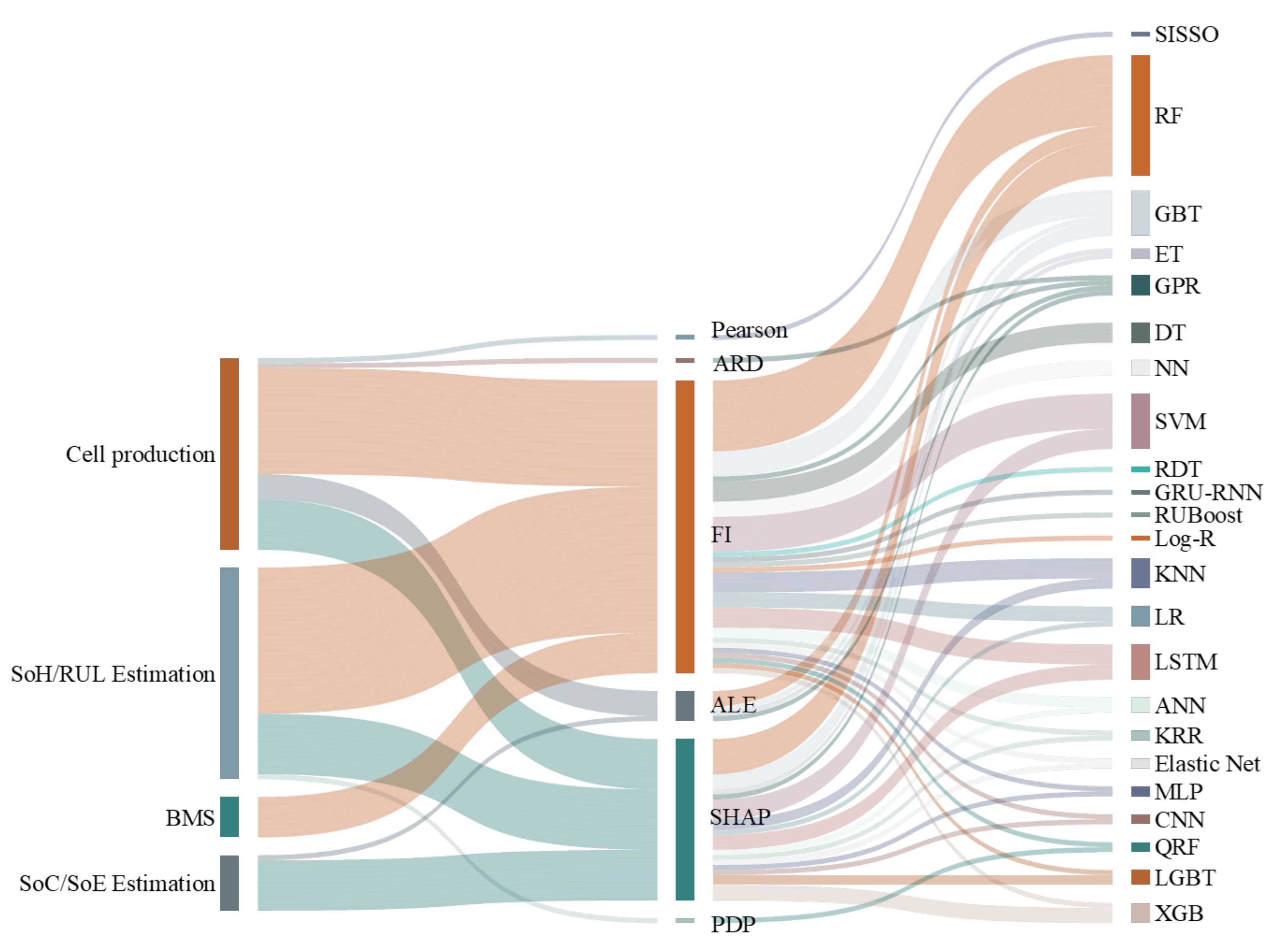
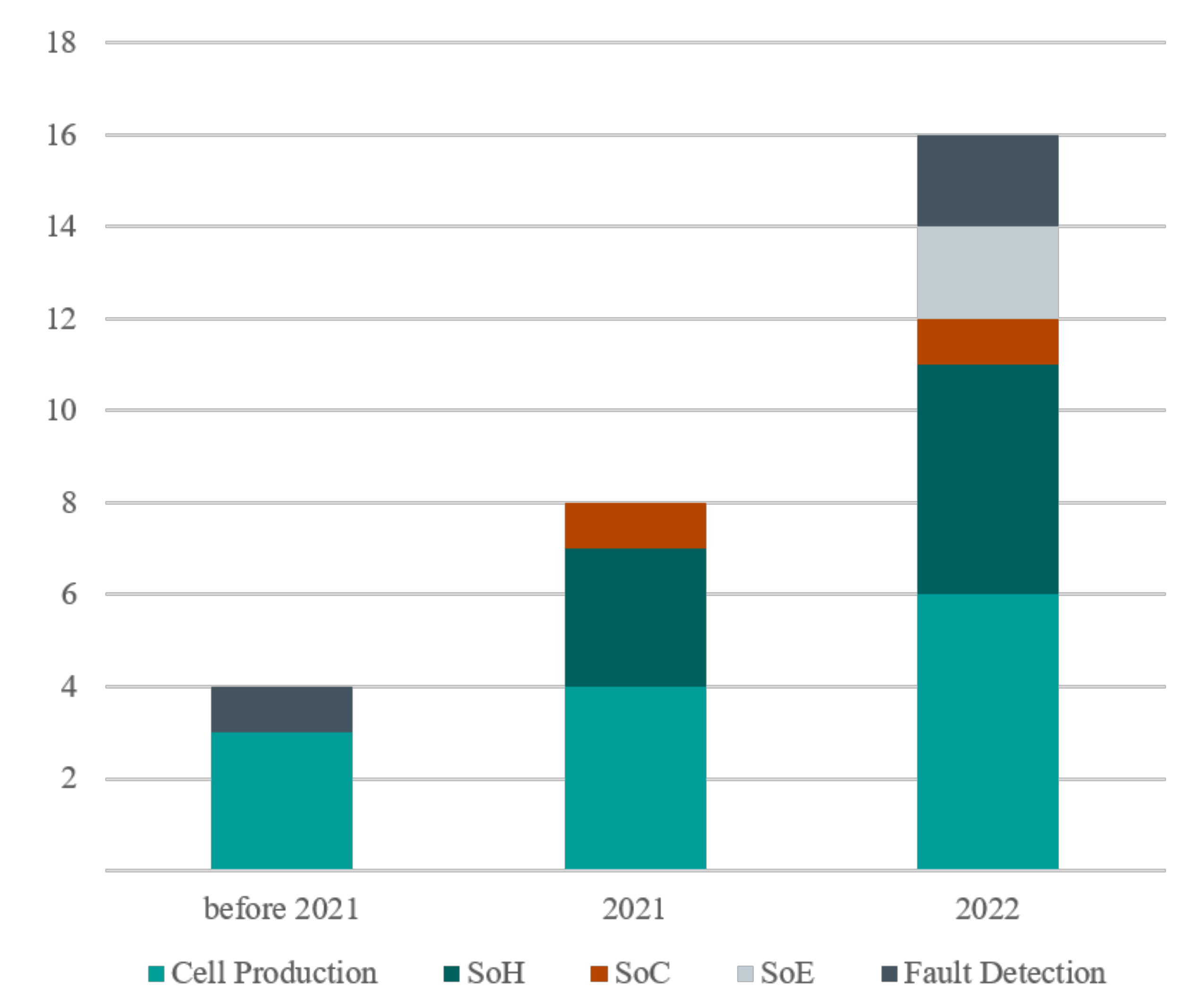
Compared to the large number of studies in the domain of lithium–ion batteries that take advantage of data-driven approaches and mainly machine learning techniques for modelling, characterisation, fault detection and diagnosis, control, and management of those in manufacturing or applications, the number of the research studies that take it to the next step and focus on the explanation and interpretation is critically low. Dividing the research subjects of battery and electrification applications into three main sections of battery cell production, battery state estimation, and modelling, and battery management systems and control, the largest number of works can be found on battery cell production and battery health estimation or life prediction. This leaves the SoC and SoE estimation and the control algorithms via XML in the last place.

-

Focusing on the cell production research and based on the summary given by Table 1, it is evident that not all process steps have received the same level of attention in the literature. At this area, formation and coating processes are most often described by XML techniques (61.5% and 53%, respectively). This is followed by calendering and mixing processes with 30% and 23% of the total papers, respectively. Specifically, the drying process in electrode manufacturing has not been addressed so far in the XML battery research field. Additionally, the utilisation of XML methods throughout the entire process chain, including cell assembly and finalisation, has received limited attention.

-

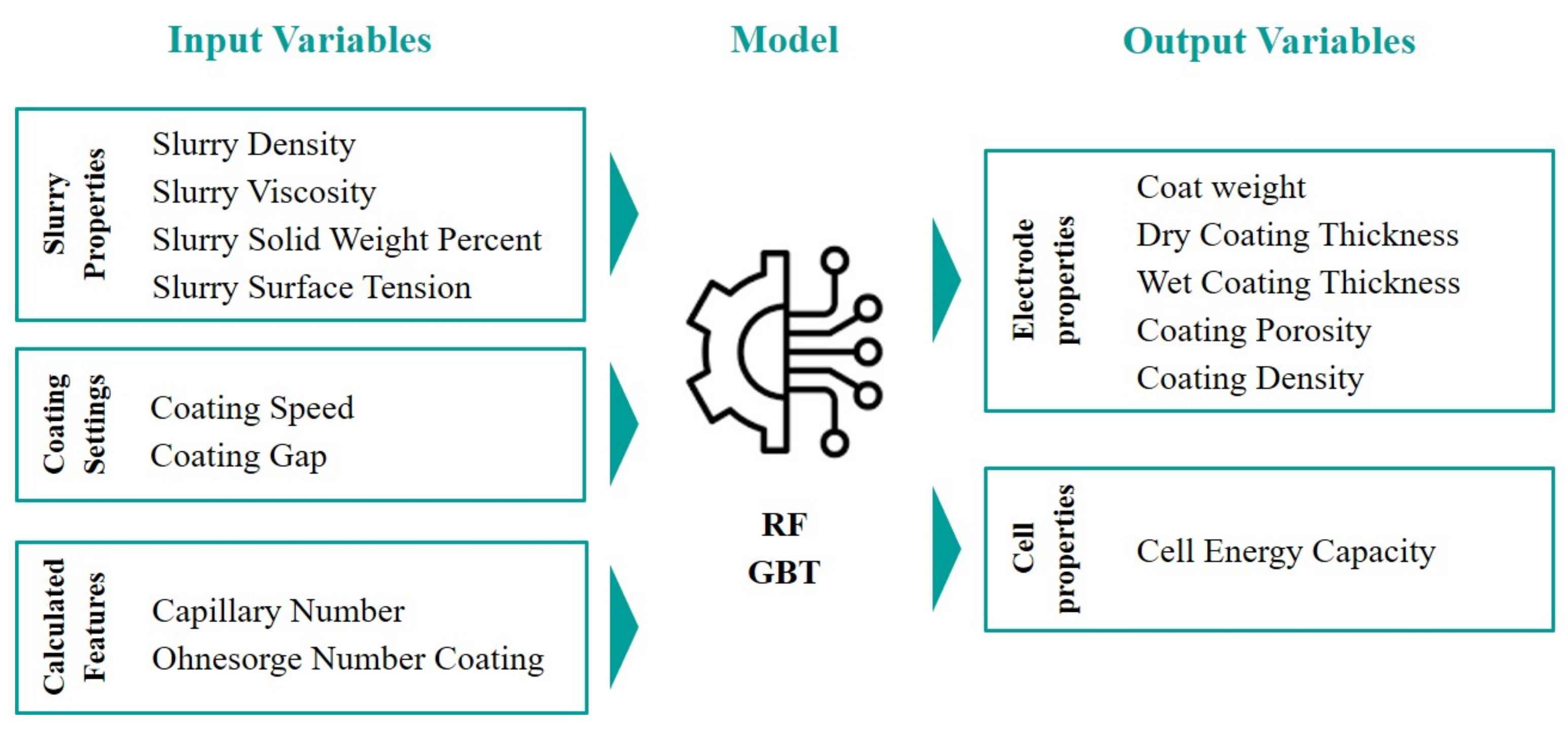
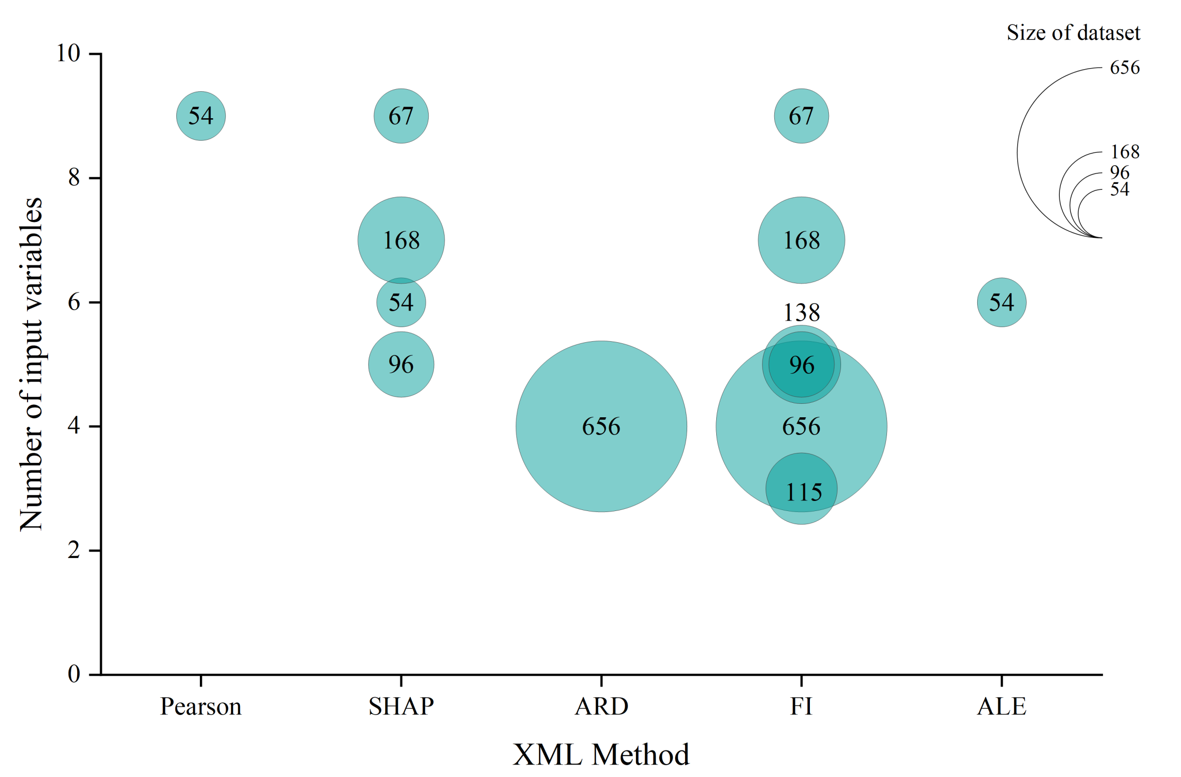
One of the major advantages of XML techniques is to provide transparency and insights into the model. Given the intricate nature of the battery cell production chain, particularly in electrode manufacturing, where a high number of interrelated parameters are involved [139], this advantage is invaluable in terms of gaining profound process understanding and accelerating decision-making for process optimisation. Figure 8 shows the number of input variables in combination with the size of the dataset for studies in electrode manufacturing using XML methods. The majority of the studies are based on four to five input variables. However, the range varies from a minimum of three to a maximum of nine input variables. As the number of variables rises, the use of XML methods becomes increasingly valuable for overarching process optimisations. The majority of studies with a high number of variables revolve around variables from formulations. The current literature still lacks a comprehensive exploration of variations in production processes. However, it is essential to acknowledge that conducting a comprehensive analysis of battery cell production can be costly and require significant effort. To tackle this challenge, a combination of optimal DoE [140] and XML methods can be adopted, enabling a comprehensive cross-process analysis and optimisation.

-

Among the reviewed articles, and as summarised in Table 3, feature importance is the most common method used for explainability, having 62% of the articles dedicated to it. This leaves a smaller percentage of 30% and 15% to Shapley-based analysis and dependencies such as ALE and PDP. A total of 25% of the works address more than one explainability technique. It is worth mentioning that some of the other explainability techniques are not used at all in this content, for example, local interpretable model-agnostic explanations (LIMEs). This is also the case for the techniques of data importance analysis such as Data Shapely and Counterfactual explainability that were introduced in Section 3. Data Shapley is in particular very important to evaluate the value of the data; it helps to identify the most significant and contribution data points to the decisions/prediction and helps reduce the data size as a large dataset does not necessarily mean a more efficient one.

-

Through the review process of this work, it was identified that some studies refer to linera correlation analysis (mainly Pearson method) as a form of explanation for the models. While this is conceptually correct and the strength of the correlations between the variables can be used as a form of feature importance, the novel definition of XML would not categorise this type of analysis as an explanation [28].

-

In general, the small ratio of works that tend to address the explainable ML is believed to be due to a number of reasons. First, while the trustworthy AI concepts, and a major technical part of it, e.g., explainability and interpretability, are rather well defined and introduced to other research communities such as health care, social sciences, and finance, it is not yet defined or put into notice in the energy or battery domain. This is a major challenge because one of the main concerns of the users and the ML models in the battery field is still struggling with confidence and trust, and part of this is due to the black-box nature of the ML techniques. Providing information about how the ML framework is making decisions or performing predictions could add to the confidence of the users when attempting using those for new datasets.

7.2. Future Prospects

Figure 9 provides an overview of articles published over the years in different battery research domains, adopting XML techniques. The figure confirms that XML is an emerging trend in different fields of battery research, with the number of publications growing from four articles before 2021 to 16 in 2022. This figure does not include the articles from 2023, as the inspection was conducted in May 2023, and the numbers have been limited for this period of time. It is also worth noting that, as of 2022, all five different research fields in the battery value chain are represented in the XML literature. Despite these advancements, there are still various aspects that need to be addressed for increasing the explainability of ML techniques in the battery field.

• All of the existing works on the XML are dedicated to lithium–ion batteries, and there are no studies that focus on the explainability of ML models for what is called “beyond lithium–ion” [141]. This is a serious challenge as the growing demand for the energy capacity and safety of rechargeable cells for electrification of transportation systems and e-mobility have made it clear that other types of cells (e.g., all-solid-state batteries, sodium–ion batteries) need to find their way into the market.
• What is investigated and proposed in the explainable ML for the battery field up to now has mainly been aimed to provide recommendations and analysis regarding the results. This means that XML has not yet been used for optimisation and improvement purposes in any of the mentioned categories of production, state estimation, or control. Taking the explanation results into account in the form of a feedback control scheme is something that is missing in the battery field and needs further investments.
• Explainability and interpretability are only one of the aspects of the trustworthy AI methods, as described in Section 1. This work has made an attempt to address this particular aspect, specifically for LiB research. However, other dimensions of trustworthiness have yet to be explored by the LiB research community. It is essential to investigate, address, and provide clarity on these aspects to enhance the trust and applicability of such models.
• As the summary of the findings in the Table 3 shows, there is a shortage of the research resources dedicated to the explanations of the NNs for modelling and prediction of lithium–ion batteries. Although the NNs has been widely adopted, especially in performance prediction of batteries [142,143], they are not yet equipped with the explainability techniques and this is definitely a clear area for improvement.
• One particular area of modelling and optimisation in the lithium–ion batteries is based on image data of its microstructure. Example studies are [144] for micro-structure reconstruction and [145] for capturing the impact of the cells’ mesostructure on its performance. There is also research that addresses the challenge of image segmentation (to separate/classify the active material particles, the binder, and the pores) before any modelling activities are performed [146,147]. While image-based studies are approached via various techniques of ML or deep learning (DL), the models’ or algorithms’ explainability has not yet been addressed. Such studies are crucial to understanding why a particular section of the images is identified to belong to a specific class or why a particular connection has been identified between the micro-structures’ characteristics and the cells’ performance.
• The previous point mentioned regarding the image data and explainability is also a missing area for the time series data in the battery field. This review has already listed a number of studies that have performed predictions of the state of health based on the cycling data of the cells at various conditions; however, they mainly use feature importance as explainability techniques and none of the particular techniques specific to the time series have been reported there [148]. Techniques based on back-propagation [149] and perturbation [150], which are tailored to the data type, are much more efficient in this case and could reveal interesting relations between factors and responses.
• As machine learning and artificial intelligent techniques are under continuous update and progress to make them adaptable to various datasets, the creation and development of novel explainability methods is critical. The basic requirement of testing such methods is the availability of a benchmark dataset that the methods can be tested against so the investigations show their advantages and weaknesses. Unfortunately, the lithium–ion battery community has not yet presented such benchmark dataset for this purpose. In fact, although there exist various open data resources such as [151,152,153], none of those have the ground truth explanation results reported in them, so there exists no case to compare the performance of the methods against that. Planning and creating such datasets is one future aspect that could be approached by the battery community in the future.

References

1. Hesse, H.C.; Schimpe, M.; Kucevic, D.; Jossen, A. Lithium-ion battery storage for the grid—A review of stationary battery storage system design tailored for applications in modern power grids. Energies 2017, 10, 2107. [Google Scholar] [CrossRef]
2. BASF. 2021. Available online: https://www.basf.com/cn/zh.html (accessed on 27 May 2023).
3. Lombardo, T.; Duquesnoy, M.; El-Bouysidy, H.; Årén, F.; Gallo-Bueno, A.; Jørgensen, P.B.; Bhowmik, A.; Demortière, A.; Ayerbe, E.; Alcaide, F.; et al. Artificial intelligence applied to battery research: Hype or reality? Chem. Rev. 2021, 122, 10899–10969. [Google Scholar] [CrossRef]
4. Li, Y.; Liu, K.; Foley, A.M.; Zülke, A.; Berecibar, M.; Nanini-Maury, E.; Van Mierlo, J.; Hoster, H.E. Data-driven health estimation and lifetime prediction of lithium-ion batteries: A review. Renew. Sustain. Energy Rev. 2019, 113, 109254. [Google Scholar] [CrossRef]
5. European Union. Ethics Guidelines for Trustworthy AI. 2019. Available online: https://digital-strategy.ec.europa.eu/en/library/ethics-guidelines-trustworthy-ai (accessed on 10 July 2023).
6. Li, B.; Qi, P.; Liu, B.; Di, S.; Liu, J.; Pei, J.; Yi, J.; Zhou, B. Trustworthy AI: From principles to practices. ACM Comput. Surv. 2023, 55, 1–46. [Google Scholar] [CrossRef]
7. Kaur, D.; Uslu, S.; Rittichier, K.J.; Durresi, A. Trustworthy artificial intelligence: A review. ACM Comput. Surv. (CSUR) 2022, 55, 1–38. [Google Scholar] [CrossRef]
8. Adadi, A.; Berrada, M. Peeking inside the black-box: A survey on explainable artificial intelligence (XAI). IEEE Access 2018, 6, 52138–52160. [Google Scholar] [CrossRef]
9. Haghi, S.; Hidalgo, M.F.V.; Niri, M.F.; Daub, R.; Marco, J. Machine Learning in Lithium-Ion Battery Cell Production: A Comprehensive Mapping Study. Batter. Supercaps 2023, 6, e202300046. [Google Scholar] [CrossRef]
10. Russell, S.; Norvig, P. AI a modern approach. Learning 2005, 2, 4. [Google Scholar]
11. Bishop, C.M.; Nasrabadi, N.M. Pattern Recognition and Machine Learning; Springer: Berlin/Heidelberg, Germany, 2006; Volume 4. [Google Scholar]
12. Alloghani, M.; Al-Jumeily, D.; Mustafina, J.; Hussain, A.; Aljaaf, A. Supervised and Unsupervised Learning for Data Science; Springer: Berlin/Heidelberg, Germany, 2020. [Google Scholar]
13. Kwade, A.; Haselrieder, W.; Leithoff, R.; Modlinger, A.; Dietrich, F.; Droeder, K. Current status and challenges for automotive battery production technologies. Nat. Energy 2018, 3, 290–300. [Google Scholar] [CrossRef]
14. Grant, P.S.; Greenwood, D.; Pardikar, K.; Smith, R.; Entwistle, T.; Middlemiss, L.A.; Murray, G.; Cussen, S.A.; Lain, M.J.; Capener, M.; et al. Roadmap on Li-ion battery manufacturing research. J. Physics Energy 2022, 4, 042006. [Google Scholar] [CrossRef]
15. Arrieta, A.B.; Díaz-Rodríguez, N.; Del Ser, J.; Bennetot, A.; Tabik, S.; Barbado, A.; García, S.; Gil-López, S.; Molina, D.; Benjamins, R.; et al. Explainable Artificial Intelligence (XAI): Concepts, taxonomies, opportunities and challenges toward responsible AI. Inf. Fusion 2020, 58, 82–115. [Google Scholar] [CrossRef]
16. Guidotti, R.; Monreale, A.; Ruggieri, S.; Turini, F.; Giannotti, F.; Pedreschi, D. A survey of methods for explaining black box models. ACM Comput. Surv. (CSUR) 2018, 51, 1–42. [Google Scholar] [CrossRef]
17. Huang, X.; Jin, G.; Ruan, W. Machine Learning Safety; Springer Nature: Berlin/Heidelberg, Germany, 2023. [Google Scholar]
18. Hawkins, R.; Paterson, C.; Picardi, C.; Jia, Y.; Calinescu, R.; Habli, I. Assurance of Machine Learning for use in Autonomous Systems (AMLAS). Available online: https://www.york.ac.uk/assuring-autonomy/guidance/amlas (accessed on 30 April 2023).
19. Hawkins, R.; Osborne, M.; Parsons, M.; Nicholson, M.; McDermid, J.; Habli, I. Guidance on the Safety Assurance of Autonomous Systems in Complex Environments (SACE). arXiv 2022, arXiv:2208.00853. [Google Scholar]
20. Doshi-Velez, F.; Kim, B. Towards a rigorous science of interpretable machine learning. arXiv 2017, arXiv:1702.08608. [Google Scholar]
21. Lipton, Z.C. The mythos of model interpretability: In machine learning, the concept of interpretability is both important and slippery. Queue 2018, 16, 31–57. [Google Scholar] [CrossRef]
22. Belle, V.; Papantonis, I. Principles and practice of explainable machine learning. Front. Big Data 2021, 4, 39. [Google Scholar] [CrossRef]
23. EUregulatin. 2023. Available online: https://commission.europa.eu/strategy-and-policy/priorities-2019-2024_en (accessed on 27 May 2023).
24. Young, S.R.; Rose, D.C.; Karnowski, T.P.; Lim, S.H.; Patton, R.M. Optimizing deep learning hyper-parameters through an evolutionary algorithm. In Proceedings of the Workshop on Machine Learning in High-Performance Computing Environments, St. Louis, MO, USA, 15 November 2015; pp. 1–5. [Google Scholar]
25. Rossi, F. Building trust in artificial intelligence. J. Int. Aff. 2018, 72, 127–134. [Google Scholar]
26. Spinner, T.; Schlegel, U.; Schäfer, H.; El-Assady, M. explAIner: A visual analytics framework for interactive and explainable machine learning. IEEE Trans. Vis. Comput. Graph. 2019, 26, 1064–1074. [Google Scholar] [CrossRef]
27. Friedman, J.H. Greedy function approximation: A gradient boosting machine. Ann. Stat. 2001, 29, 1189–1232. [Google Scholar] [CrossRef]
28. Molnar, C. Interpretable Machine Learning. Available online: https://www.lulu.com/ (accessed on 30 June 2023).
29. Apley, D.W.; Zhu, J. Visualizing the effects of predictor variables in black box supervised learning models. J. R. Stat. Soc. Ser. B Stat. Methodol. 2020, 82, 1059–1086. [Google Scholar] [CrossRef]
30. Gkolemis, V.; Dalamagas, T.; Diou, C. DALE: Differential Accumulated Local Effects for efficient and accurate global explanations. In Proceedings of the Asian Conference on Machine Learning, PMLR, Bangkok, Thailand, 18–20 November 2023; pp. 375–390. [Google Scholar]
31. Breiman, L. Random forests. Mach. Learn. 2001, 45, 5–32. [Google Scholar] [CrossRef]
32. Altmann, A.; Toloşi, L.; Sander, O.; Lengauer, T. Permutation importance: A corrected feature importance measure. Bioinformatics 2010, 26, 1340–1347. [Google Scholar] [CrossRef] [PubMed]
33. Auret, L.; Aldrich, C. Empirical comparison of tree ensemble variable importance measures. Chemom. Intell. Lab. Syst. 2011, 105, 157–170. [Google Scholar] [CrossRef]
34. Díaz-Uriarte, R.; Alvarez de Andrés, S. Gene selection and classification of microarray data using random forest. BMC Bioinform. 2006, 7, 3. [Google Scholar] [CrossRef]
35. Ishwaran, H. Variable importance in binary regression trees and forests. Electron. J. Statist. 2007, 1, 519–537. [Google Scholar] [CrossRef]
36. Rodenburg, W.; Heidema, A.G.; Boer, J.M.; Bovee-Oudenhoven, I.M.; Feskens, E.J.; Mariman, E.C.; Keijer, J. A framework to identify physiological responses in microarray-based gene expression studies: Selection and interpretation of biologically relevant genes. Physiol. Genom. 2008, 33, 78–90. [Google Scholar] [CrossRef]
37. Strobl, C.; Boulesteix, A.L.; Kneib, T.; Augustin, T.; Zeileis, A. Conditional variable importance for random forests. BMC Bioinform. 2008, 9, 307. [Google Scholar] [CrossRef]
38. Nembrini, S.; König, I.R.; Wright, M.N. The revival of the Gini importance? Bioinformatics 2018, 34, 3711–3718. [Google Scholar] [CrossRef]
39. Breiman, L.; Friedman, J.; Stone, C.J.; Olshen, R.A. Classification and Regression Trees; CRC Press: Boca Raton, FL, USA, 1984. [Google Scholar]
40. Hastie, T.; Tibshirani, R.; Friedman, J.H.; Friedman, J.H. The Elements of Statistical Learning: Data Mining, Inference, and Prediction; Springer: Berlin/Heidelberg, Germany, 2009; Volume 2. [Google Scholar]
41. Kukreja, S.L.; Löfberg, J.; Brenner, M.J. A least absolute shrinkage and selection operator (LASSO) for nonlinear system identification. IFAC Proc. Vol. 2006, 39, 814–819. [Google Scholar] [CrossRef]
42. Lundberg, S.M.; Erion, G.G.; Lee, S.I. Consistent individualized feature attribution for tree ensembles. arXiv 2018, arXiv:1802.03888. [Google Scholar]
43. Saabas, A. Interpreting random forests. Diving Data 2014, 24. [Google Scholar]
44. Hastie, T.; Tibshirani, R.; Friedman, J. The Elements of Statistical Learning; Springer Series in Statistics; Springer: New York, NY, USA, 2001. [Google Scholar]
45. Chebrolu, S.; Abraham, A.; Thomas, J.P. Feature deduction and ensemble design of intrusion detection systems. Comput. Secur. 2005, 24, 295–307. [Google Scholar] [CrossRef]
46. Huynh-Thu, V.A.; Irrthum, A.; Wehenkel, L.; Geurts, P. Inferring regulatory networks from expression data using tree-based methods. PLoS ONE 2010, 5, e12776. [Google Scholar] [CrossRef] [PubMed]
47. Sandri, M.; Zuccolotto, P. A bias correction algorithm for the Gini variable importance measure in classification trees. J. Comput. Graph. Stat. 2008, 17, 611–628. [Google Scholar] [CrossRef]
48. Chen, T.; Guestrin, C. Xgboost: A scalable tree boosting system. In Proceedings of the 22nd ACM SIGKDD International Conference on Knowledge Discovery and Data Mining, San Francisco, CA, USA, 13–17 August 2016; pp. 785–794. [Google Scholar]
49. Lundberg, S.M.; Erion, G.; Chen, H.; DeGrave, A.; Prutkin, J.M.; Nair, B.; Katz, R.; Himmelfarb, J.; Bansal, N.; Lee, S.I. From local explanations to global understanding with explainable AI for trees. Nat. Mach. Intell. 2020, 2, 2522–5839. [Google Scholar] [CrossRef]
50. Lundberg, S.M.; Nair, B.; Vavilala, M.S.; Horibe, M.; Eisses, M.J.; Adams, T.; Liston, D.E.; Low, D.K.W.; Newman, S.F.; Kim, J.; et al. Explainable machine-learning predictions for the prevention of hypoxaemia during surgery. Nat. Biomed. Eng. 2018, 2, 749. [Google Scholar] [CrossRef] [PubMed]
51. Cohen, I.; Huang, Y.; Chen, J.; Benesty, J.; Benesty, J.; Chen, J.; Huang, Y.; Cohen, I. Pearson correlation coefficient. Noise Reduct. Speech Process. 2009, 2, 1–4. [Google Scholar]
52. Faraji Niri, M.; Apachitei, G.; Lain, M.; Copley, M.; Marco, J. The Impact of Calendering Process Variables on the Impedance and Capacity Fade of Lithium-Ion Cells: An Explainable Machine Learning Approach. Energy Technol. 2022, 10, 2200893. [Google Scholar] [CrossRef]
53. Ghorbani, A.; Zou, J. Data shapley: Equitable valuation of data for machine learning. In Proceedings of the International Conference on Machine Learning. PMLR, Long Beach, CA, USA, 9–15 June 2019; pp. 2242–2251. [Google Scholar]
54. Wachter, S.; Mittelstadt, B.; Russell, C. Counterfactual explanations without opening the black box: Automated decisions and the GDPR. Harv. JL Tech. 2017, 31, 841. [Google Scholar] [CrossRef]
55. Karimi, A.H.; Schölkopf, B.; Valera, I. Algorithmic recourse: From counterfactual explanations to interventions. In Proceedings of the 2021 ACM Conference on Fairness, Accountability, and Transparency, Toronto, ON, Canada, 3–10 March 2021; pp. 353–362. [Google Scholar]
56. Verma, S.; Boonsanong, V.; Hoang, M.; Hines, K.E.; Dickerson, J.P.; Shah, C. Counterfactual explanations and algorithmic recourses for machine learning: A review. arXiv 2020, arXiv:2010.10596. [Google Scholar]
57. Stepin, I.; Alonso, J.M.; Catala, A.; Pereira-Fariña, M. A survey of contrastive and counterfactual explanation generation methods for explainable artificial intelligence. IEEE Access 2021, 9, 11974–12001. [Google Scholar] [CrossRef]
58. Sokol, K.; Flach, P.A. Counterfactual Explanations of Machine Learning Predictions: Opportunities and Challenges for AI Safety. SafeAI@ AAAI 2019, 2301, 1–4. [Google Scholar]
59. Baron, S. Explainable AI and Causal Understanding: Counterfactual Approaches Considered. Minds Mach. 2023, 33, 347–377. [Google Scholar] [CrossRef]
60. De Toni, G.; Lepri, B.; Passerini, A. Synthesizing explainable counterfactual policies for algorithmic recourse with program synthesis. Mach. Learn. 2023, 112, 1389–1409. [Google Scholar] [CrossRef]
61. Brughmans, D.; Melis, L.; Martens, D. Disagreement amongst counterfactual explanations: How transparency can be deceptive. arXiv 2023, arXiv:2304.12667. [Google Scholar]
62. Bhatt, U.; Xiang, A.; Sharma, S.; Weller, A.; Taly, A.; Jia, Y.; Ghosh, J.; Puri, R.; Moura, J.M.; Eckersley, P. Explainable machine learning in deployment. In Proceedings of the 2020 Conference on Fairness, Accountability, and Transparency, Barcelona, Spain, 27–30 June 2020; pp. 648–657. [Google Scholar]
63. Ghorbani, A.; Abid, A.; Zou, J. Interpretation of neural networks is fragile. In Proceedings of the AAAI Conference on Artificial Intelligence, Honolulu, HI, USA, 27 January–1 February 2019; Volume 33, pp. 3681–3688. [Google Scholar]
64. Slack, D.; Hilgard, S.; Jia, E.; Singh, S.; Lakkaraju, H. Fooling lime and shap: Adversarial attacks on post hoc explanation methods. In Proceedings of the AAAI/ACM Conference on AI, Ethics, and Society, New York, NY, USA, 8–10 August 2020; pp. 180–186. [Google Scholar]
65. Li, J.; Fleetwood, J.; Hawley, W.B.; Kays, W. From materials to cell: State-of-the-art and prospective technologies for lithium-ion battery electrode processing. Chem. Rev. 2021, 122, 903–956. [Google Scholar] [CrossRef]
66. Liu, Y.; Zhang, R.; Wang, J.; Wang, Y. Current and future lithium-ion battery manufacturing. IScience 2021, 24, 102332. [Google Scholar] [CrossRef]
67. Wang, G.; Fearn, T.; Wang, T.; Choy, K.L. Machine-Learning Approach for Predicting the Discharging Capacities of Doped Lithium Nickel–Cobalt–Manganese Cathode Materials in Li-Ion Batteries. ACS Cent. Sci. 2021, 7, 1551–1560. [Google Scholar] [CrossRef]
68. Liu, K.; Hu, X.; Meng, J.; Guerrero, J.M.; Teodorescu, R. RUBoost-based ensemble machine learning for electrode quality classification in Li-ion battery manufacturing. IEEE/ASME Trans. Mechatronics 2021, 27, 2474–2483. [Google Scholar] [CrossRef]
69. Rynne, O.; Dubarry, M.; Molson, C.; Nicolas, E.; Lepage, D.; Prebe, A.; Ayme-Perrot, D.; Rochefort, D.; Dolle, M. Exploiting materials to their full potential, a Li-ion battery electrode formulation optimization study. ACS Appl. Energy Mater. 2020, 3, 2935–2948. [Google Scholar] [CrossRef]
70. Niri, M.F.; Apachitei, G.; Lain, M.; Copley, M.; Marco, J. Machine learning for investigating the relative importance of electrodes’ N: P areal capacity ratio in the manufacturing of lithium-ion battery cells. J. Power Sources 2022, 549, 232124. [Google Scholar] [CrossRef]
71. Niri, M.F.; Reynolds, C.; Ramírez, L.A.R.; Kendrick, E.; Marco, J. Systematic analysis of the impact of slurry coating on manufacture of Li-ion battery electrodes via explainable machine learning. Energy Storage Mater. 2022, 51, 223–238. [Google Scholar] [CrossRef]
72. Sandri, M.; Zuccolotto, P. Analysis and correction of bias in total decrease in node impurity measures for tree-based algorithms. Stat. Comput. 2010, 20, 393–407. [Google Scholar] [CrossRef]
73. Xu, Z.; Huang, G.; Weinberger, K.Q.; Zheng, A.X. Gradient boosted feature selection. In Proceedings of the 20th ACM SIGKDD International Conference on Knowledge Discovery and Data Mining, New York, NY, USA, 24–27 August 2014; pp. 522–531. [Google Scholar]
74. Cunha, R.P.; Lombardo, T.; Primo, E.N.; Franco, A.A. Artificial intelligence investigation of NMC cathode manufacturing parameters interdependencies. Batter. Supercaps 2020, 3, 60–67. [Google Scholar] [CrossRef]
75. Liu, K.; Hu, X.; Zhou, H.; Tong, L.; Widanage, W.D.; Marco, J. Feature analyses and modeling of lithium-ion battery manufacturing based on random forest classification. IEEE/ASME Trans. Mechatronics 2021, 26, 2944–2955. [Google Scholar] [CrossRef]
76. Liu, K.; Wei, Z.; Yang, Z.; Li, K. Mass load prediction for lithium-ion battery electrode clean production: A machine learning approach. J. Clean. Prod. 2021, 289, 125159. [Google Scholar] [CrossRef]
77. Liu, K.; Peng, Q.; Li, K.; Chen, T. Data-based interpretable modeling for property forecasting and sensitivity analysis of Li-ion battery electrode. Automot. Innov. 2022, 5, 121–133. [Google Scholar] [CrossRef]
78. Niri, M.F.; Liu, K.; Apachitei, G.; Román-Ramírez, L.A.; Lain, M.; Widanage, D.; Marco, J. Quantifying key factors for optimised manufacturing of Li-ion battery anode and cathode via artificial intelligence. Energy AI 2022, 7, 100129. [Google Scholar] [CrossRef]
79. Liu, K.; Niri, M.F.; Apachitei, G.; Lain, M.; Greenwood, D.; Marco, J. Interpretable machine learning for battery capacities prediction and coating parameters analysis. Control Eng. Pract. 2022, 124, 105202. [Google Scholar] [CrossRef]
80. Faraji Niri, M.; Liu, K.; Apachitei, G.; Roman Ramirez, L.; Widanage, W.D.; Marco, J. Data mining for quality prediction of battery in manufacturing process: Cathode coating process. In Proceedings of the 12th International Conference on Applied Energy, Bangkok, Thiland, 29 November–2 December 2020; Volume 11. [Google Scholar]
81. Niri, M.F.; Liu, K.; Apachitei, G.; Ramirez, L.R.; Lain, M.; Widanage, D.; Marco, J. Machine learning for optimised and clean Li-ion battery manufacturing: Revealing the dependency between electrode and cell characteristics. J. Clean. Prod. 2021, 324, 129272. [Google Scholar] [CrossRef]
82. Duquesnoy, M.; Lombardo, T.; Chouchane, M.; Primo, E.N.; Franco, A.A. Data-driven assessment of electrode calendering process by combining experimental results, in silico mesostructures generation and machine learning. J. Power Sources 2020, 480, 229103. [Google Scholar] [CrossRef]
83. Turetskyy, A.; Thiede, S.; Thomitzek, M.; von Drachenfels, N.; Pape, T.; Herrmann, C. Toward data-driven applications in lithium-ion battery cell manufacturing. Energy Technol. 2020, 8, 1900136. [Google Scholar] [CrossRef]
84. Turetskyy, A.; Wessel, J.; Herrmann, C.; Thiede, S. Data-driven cyber-physical system for quality gates in lithium-ion battery cell manufacturing. Procedia CIRP 2020, 93, 168–173. [Google Scholar] [CrossRef]
85. Chang, W.Y. The state of charge estimating methods for battery: A review. Int. Sch. Res. Not. 2013, 2013, 1–7. [Google Scholar] [CrossRef]
86. Shrivastava, P.; Soon, T.K.; Idris, M.Y.I.B.; Mekhilef, S. Overview of model-based online state-of-charge estimation using Kalman filter family for lithium-ion batteries. Renew. Sustain. Energy Rev. 2019, 113, 109233. [Google Scholar] [CrossRef]
87. Shu, X.; Shen, S.; Shen, J.; Zhang, Y.; Li, G.; Chen, Z.; Liu, Y. State of health prediction of lithium-ion batteries based on machine learning: Advances and perspectives. Iscience 2021, 24, 103265. [Google Scholar] [CrossRef] [PubMed]
88. Zenati, A.; Desprez, P.; Razik, H.; Rael, S. A methodology to assess the State of Health of lithium-ion batteries based on the battery’s parameters and a Fuzzy Logic System. In Proceedings of the 2012 IEEE International Electric Vehicle Conference, Greenville, SC, USA, 4–8 March 2012; pp. 1–6. [Google Scholar]
89. Dubarry, M.; Qin, N.; Brooker, P. Calendar aging of commercial Li-ion cells of different chemistries—A review. Curr. Opin. Electrochem. 2018, 9, 106–113. [Google Scholar] [CrossRef]
90. Vetter, J.; Novák, P.; Wagner, M.R.; Veit, C.; Möller, K.C.; Besenhard, J.; Winter, M.; Wohlfahrt-Mehrens, M.; Vogler, C.; Hammouche, A. Ageing mechanisms in lithium-ion batteries. J. Power Sources 2005, 147, 269–281. [Google Scholar] [CrossRef]
91. Heiskanen, S.K.; Kim, J.; Lucht, B.L. Generation and evolution of the solid electrolyte interphase of lithium-ion batteries. Joule 2019, 3, 2322–2333. [Google Scholar] [CrossRef]
92. Lin, N.; Jia, Z.; Wang, Z.; Zhao, H.; Ai, G.; Song, X.; Bai, Y.; Battaglia, V.; Sun, C.; Qiao, J.; et al. Understanding the crack formation of graphite particles in cycled commercial lithium-ion batteries by focused ion beam-scanning electron microscopy. J. Power Sources 2017, 365, 235–239. [Google Scholar] [CrossRef]
93. Faraji-Niri, M.; Rashid, M.; Sansom, J.; Sheikh, M.; Widanage, D.; Marco, J. Accelerated state of health estimation of second life lithium-ion batteries via electrochemical impedance spectroscopy tests and machine learning techniques. J. Energy Storage 2023, 58, 106295. [Google Scholar] [CrossRef]
94. Haifeng, D.; Xuezhe, W.; Zechang, S. A new SOH prediction concept for the power lithium-ion battery used on HEVs. In Proceedings of the 2009 IEEE Vehicle Power and Propulsion Conference, Dearborn, MI, USA, 7–11 September 2009; pp. 1649–1653. [Google Scholar]
95. Zhu, J.; Mathews, I.; Ren, D.; Li, W.; Cogswell, D.; Xing, B.; Sedlatschek, T.; Kantareddy, S.N.R.; Yi, M.; Gao, T.; et al. End-of-life or second-life options for retired electric vehicle batteries. Cell Rep. Phys. Sci. 2021, 2, 100537. [Google Scholar] [CrossRef]
96. Lee, G.; Kim, J.; Lee, C. State-of-health estimation of Li-ion batteries in the early phases of qualification tests: An interpretable machine learning approach. Expert Syst. Appl. 2022, 197, 116817. [Google Scholar] [CrossRef]
97. Mawonou, K.S.; Eddahech, A.; Dumur, D.; Beauvois, D.; Godoy, E. State-of-health estimators coupled to a random forest approach for lithium-ion battery aging factor ranking. J. Power Sources 2021, 484, 229154. [Google Scholar] [CrossRef]
98. Jiang, F.; He, Y.; Gao, D.; Zhou, Y.; Liu, W.; Yan, L.; Peng, J. An Accurate and Interpretable Lifetime Prediction Method for Batteries using Extreme Gradient Boosting Tree and TreeExplainer. In Proceedings of the 2021 IEEE 23rd Int Conf on High Performance Computing & Communications; 7th Int Conf on Data Science & Systems; 19th Int Conf on Smart City; 7th Int Conf on Dependability in Sensor, Cloud & Big Data Systems & Application (HPCC/DSS/SmartCity/DependSys), Haikou, China, 20–22 December 2021; pp. 1042–1048. [Google Scholar]
99. Li, G.; Li, B.; Li, C.; Wang, S. State-of-health rapid estimation for lithium-ion battery based on an interpretable stacking ensemble model with short-term voltage profiles. Energy 2023, 263, 126064. [Google Scholar] [CrossRef]
100. Granado, L.; Ben-Marzouk, M.; Saenz, E.S.; Boukal, Y.; Jugé, S. Machine learning predictions of lithium-ion battery state-of-health for eVTOL applications. J. Power Sources 2022, 548, 232051. [Google Scholar] [CrossRef]
101. Zhang, H.; Su, Y.; Altaf, F.; Wik, T.; Gros, S. Interpretable Battery Cycle Life Range Prediction Using Early Cell Degradation Data. IEEE Trans. Transp. Electrif. 2022, 9, 2669–2682. [Google Scholar] [CrossRef]
102. He, J.; Tian, Y.; Wu, L. A hybrid data-driven method for rapid prediction of lithium-ion battery capacity. Reliab. Eng. Syst. Saf. 2022, 226, 108674. [Google Scholar] [CrossRef]
103. Ibraheem, R.; Strange, C.; dos Reis, G. Capacity and Internal Resistance of lithium-ion batteries: Full degradation curve prediction from Voltage response at constant Current at discharge. J. Power Sources 2023, 556, 232477. [Google Scholar] [CrossRef]
104. Rouhi Ardeshiri, R.; Ma, C. Multivariate gated recurrent unit for battery remaining useful life prediction: A deep learning approach. Int. J. Energy Res. 2021, 45, 16633–16648. [Google Scholar] [CrossRef]
105. Kim, S.W.; Oh, K.Y.; Lee, S. Novel informed deep learning-based prognostics framework for on-board health monitoring of lithium-ion batteries. Appl. Energy 2022, 315, 119011. [Google Scholar] [CrossRef]
106. Wang, F.; Zhao, Z.; Zhai, Z.; Shang, Z.; Yan, R.; Chen, X. Explainability-driven model improvement for SOH estimation of lithium-ion battery. Reliab. Eng. Syst. Saf. 2023, 232, 109046. [Google Scholar] [CrossRef]
107. Rieger, L.H.; Flores, E.; Nielsen, K.F.; Norby, P.; Ayerbe, E.; Winther, O.; Vegge, T.; Bhowmik, A. Uncertainty-aware and explainable machine learning for early prediction of battery degradation trajectory. Digit. Discov. 2023, 2, 112–122. [Google Scholar] [CrossRef]
108. Lundberg, S.M.; Lee, S.I. A unified approach to interpreting model predictions. Adv. Neural Inf. Process. Syst. 2017, 30. [Google Scholar]
109. Refaeilzadeh, P.; Tang, L.; Liu, H. Cross-validation. Encycl. Database Syst. 2009, 5, 532–538. [Google Scholar]
110. Melis, G.; Kočiskỳ, T.; Blunsom, P. Mogrifier lstm. arXiv 2019, arXiv:1909.01792. [Google Scholar]
111. Saha, B.; Goebel, K. Battery Data Set. NASA AMES Prognostics Data Repository. 2007. Available online: https://www.nasa.gov/content/prognostics-center-of-excellence-data-set-repository (accessed on 10 January 2023).
112. Bole, B.; Kulkarni, C.S.; Daigle, M. Adaptation of an electrochemistry-based li-ion battery model to account for deterioration observed under randomized use. In Proceedings of the Annual Conference of the PHM Society, Xi’an, China, 15–17 August 2014; Volume 6. [Google Scholar]
113. Attia, P.M.; Grover, A.; Jin, N.; Severson, K.A.; Markov, T.M.; Liao, Y.H.; Chen, M.H.; Cheong, B.; Perkins, N.; Yang, Z.; et al. Closed-loop optimization of fast-charging protocols for batteries with machine learning. Nature 2020, 578, 397–402. [Google Scholar] [CrossRef]
114. Lu, J.; Xiong, R.; Tian, J.; Wang, C.; Hsu, C.W.; Tsou, N.T.; Sun, F.; Li, J. Battery degradation prediction against uncertain future conditions with recurrent neural network enabled deep learning. Energy Storage Mater. 2022, 50, 139–151. [Google Scholar] [CrossRef]
115. He, W.; Williard, N.; Osterman, M.; Pecht, M. Prognostics of lithium-ion batteries based on Dempster–Shafer theory and the Bayesian Monte Carlo method. J. Power Sources 2011, 196, 10314–10321. [Google Scholar] [CrossRef]
116. eVTOL. 2021. Available online: https://electrek.co/guides/evtol/ (accessed on 30 June 2023).
117. Severson, K.A.; Attia, P.M.; Jin, N.; Perkins, N.; Jiang, B.; Yang, Z.; Chen, M.H.; Aykol, M.; Herring, P.K.; Fraggedakis, D.; et al. Data-driven prediction of battery cycle life before capacity degradation. Nat. Energy 2019, 4, 383–391. [Google Scholar] [CrossRef]
118. Koenker, R.; Bassett, G., Jr. Regression quantiles. Econom. J. Econom. Soc. 1978, 33–50. [Google Scholar] [CrossRef]
119. Xiong, R.; Cao, J.; Yu, Q.; He, H.; Sun, F. Critical review on the battery state of charge estimation methods for electric vehicles. IEEE Access 2017, 6, 1832–1843. [Google Scholar] [CrossRef]
120. Marelli, S.; Corno, M. Model-based estimation of lithium concentrations and temperature in batteries using soft-constrained dual unscented Kalman filtering. IEEE Trans. Control. Syst. Technol. 2020, 29, 926–933. [Google Scholar] [CrossRef]
121. Tran, N.T.; Vilathgamuwa, M.; Li, Y.; Farrell, T.; Teague, J. State of charge estimation of lithium ion batteries using an extended single particle model and sigma-point Kalman filter. In Proceedings of the 2017 IEEE Southern Power Electronics Conference (SPEC), Puerto Varas, Chile, 4–7 December 2017; pp. 1–6. [Google Scholar]
122. Hossain, M.; Haque, M.; Arif, M.T. Kalman filtering techniques for the online model parameters and state of charge estimation of the Li-ion batteries: A comparative analysis. J. Energy Storage 2022, 51, 104174. [Google Scholar] [CrossRef]
123. He, W.; Williard, N.; Chen, C.; Pecht, M. State of charge estimation for Li-ion batteries using neural network modeling and unscented Kalman filter-based error cancellation. Int. J. Electr. Power Energy Syst. 2014, 62, 783–791. [Google Scholar] [CrossRef]
124. Chandran, V.; Patil, C.K.; Karthick, A.; Ganeshaperumal, D.; Rahim, R.; Ghosh, A. State of charge estimation of lithium-ion battery for electric vehicles using machine learning algorithms. World Electr. Veh. J. 2021, 12, 38. [Google Scholar] [CrossRef]
125. Anton, J.C.A.; Nieto, P.J.G.; Viejo, C.B.; Vilán, J.A.V. Support vector machines used to estimate the battery state of charge. IEEE Trans. Power Electron. 2013, 28, 5919–5926. [Google Scholar] [CrossRef]
126. Niri, M.F.; Bui, T.M.; Dinh, T.Q.; Hosseinzadeh, E.; Yu, T.F.; Marco, J. Remaining energy estimation for lithium-ion batteries via Gaussian mixture and Markov models for future load prediction. J. Energy Storage 2020, 28, 101271. [Google Scholar] [CrossRef]
127. Niri, M.F.; Dinh, T.Q.; Yu, T.F.; Marco, J.; Bui, T.M.N. State of power prediction for lithium-ion batteries in electric vehicles via wavelet-Markov load analysis. IEEE Trans. Intell. Transp. Syst. 2020, 22, 5833–5848. [Google Scholar] [CrossRef]
128. Hatherall, O.; Niri, M.F.; Barai, A.; Li, Y.; Marco, J. Remaining discharge energy estimation for lithium-ion batteries using pattern recognition and power prediction. J. Energy Storage 2023, 64, 107091. [Google Scholar] [CrossRef]
129. Gu, X.; See, K.; Wang, Y.; Zhao, L.; Pu, W. The sliding window and SHAP theory—an improved system with a long short-term memory network model for state of charge prediction in electric vehicle application. Energies 2021, 14, 3692. [Google Scholar] [CrossRef]
130. Shahriar, S.M.; Bhuiyan, E.A.; Nahiduzzaman, M.; Ahsan, M.; Haider, J. State of Charge Estimation for Electric Vehicle Battery Management Systems Using the Hybrid Recurrent Learning Approach with Explainable Artificial Intelligence. Energies 2022, 15, 8003. [Google Scholar] [CrossRef]
131. Burzyński, D. Useful energy prediction model of a Lithium-ion cell operating on various duty cycles. Eksploat. Niezawodność 2022, 24, 317–329. [Google Scholar] [CrossRef]
132. Nan, S.; Tu, R.; Li, T.; Sun, J.; Chen, H. From driving behavior to energy consumption: A novel method to predict the energy consumption of electric bus. Energy 2022, 261, 125188. [Google Scholar] [CrossRef]
133. Alaoui, C. Hybrid vehicle energy management using deep learning. In Proceedings of the 2019 International Conference on Intelligent Systems and Advanced Computing Sciences (ISACS), Taza, Maroc, 26–27 December 2019; pp. 1–5. [Google Scholar]
134. Samanta, A.; Chowdhuri, S.; Williamson, S.S. Machine learning-based data-driven fault detection/diagnosis of lithium-ion battery: A critical review. Electronics 2021, 10, 1309. [Google Scholar] [CrossRef]
135. Jia, Y.; Li, J.; Yao, W.; Li, Y.; Xu, J. Precise and fast safety risk classification of lithium-ion batteries based on machine learning methodology. J. Power Sources 2022, 548, 232064. [Google Scholar] [CrossRef]
136. Chen, K.; Zheng, F.; Jiang, J.; Zhang, W.; Jiang, Y.; Chen, K. Practical failure recognition model of lithium-ion batteries based on partial charging process. Energy 2017, 138, 1199–1208. [Google Scholar] [CrossRef]
137. James, G.; Witten, D.; Hastie, T.; Tibshirani, R. Statistical learning. In An Introduction to Statistical Learning: With Applications in R; Springer: Berlin/Heidelberg, Germany, 2021; pp. 15–57. [Google Scholar]
138. Xu, C.; Li, L.; Xu, Y.; Han, X.; Zheng, Y. A vehicle-cloud collaborative method for multi-type fault diagnosis of lithium-ion batteries. eTransportation 2022, 12, 100172. [Google Scholar] [CrossRef]
139. Haghi, S.; Summer, A.; Bauerschmidt, P.; Daub, R. Tailored Digitalization in Electrode Manufacturing: The Backbone of Smart Lithium-Ion Battery Cell Production. Energy Technol. 2022, 10, 2200657. [Google Scholar] [CrossRef]
140. Román-Ramírez, L.A.; Marco, J. Design of experiments applied to lithium-ion batteries: A literature review. Appl. Energy 2022, 320, 119305. [Google Scholar] [CrossRef]
141. Tian, Y.; Zeng, G.; Rutt, A.; Shi, T.; Kim, H.; Wang, J.; Koettgen, J.; Sun, Y.; Ouyang, B.; Chen, T.; et al. Promises and challenges of next-generation “beyond Li-ion” batteries for electric vehicles and grid decarbonization. Chem. Rev. 2020, 121, 1623–1669. [Google Scholar] [CrossRef] [PubMed]
142. Cui, Z.; Wang, L.; Li, Q.; Wang, K. A comprehensive review on the state of charge estimation for lithium-ion battery based on neural network. Int. J. Energy Res. 2022, 46, 5423–5440. [Google Scholar] [CrossRef]
143. Manoharan, A.; Begam, K.; Aparow, V.R.; Sooriamoorthy, D. Artificial Neural Networks, Gradient Boosting and Support Vector Machines for electric vehicle battery state estimation: A review. J. Energy Storage 2022, 55, 105384. [Google Scholar] [CrossRef]
144. Faraji Niri, M.; Mafeni Mase, J.; Marco, J. Performance Evaluation of Convolutional Auto Encoders for the Reconstruction of Li-Ion Battery Electrode Microstructure. Energies 2022, 15, 4489. [Google Scholar] [CrossRef]
145. Dahari, A.; Kench, S.; Squires, I.; Cooper, S.J. Fusion of complementary 2D and 3D mesostructural datasets using generative adversarial networks. Adv. Energy Mater. 2023, 13, 2202407. [Google Scholar] [CrossRef]
146. Müller, S.; Sauter, C.; Shunmugasundaram, R.; Wenzler, N.; De Andrade, V.; De Carlo, F.; Konukoglu, E.; Wood, V. Deep learning-based segmentation of lithium-ion battery microstructures enhanced by artificially generated electrodes. Nat. Commun. 2021, 12, 6205. [Google Scholar] [CrossRef]
147. Usseglio-Viretta, F.L.; Patel, P.; Bernhardt, E.; Mistry, A.; Mukherjee, P.; Allen, J.; Cooper, S.; Laurencin, J.; Smith, K. MATBOX: An Open-source Microstructure Analysis Toolbox for microstructure generation, segmentation, characterization, visualization, correlation, and meshing. SoftwareX 2022, 17, 100915. [Google Scholar] [CrossRef]
148. Rojat, T.; Puget, R.; Filliat, D.; Del Ser, J.; Gelin, R.; Díaz-Rodríguez, N. Explainable artificial intelligence (xai) on timeseries data: A survey. arXiv 2021, arXiv:2104.00950. [Google Scholar]
149. Ismail Fawaz, H.; Forestier, G.; Weber, J.; Idoumghar, L.; Muller, P.A. Accurate and interpretable evaluation of surgical skills from kinematic data using fully convolutional neural networks. Int. J. Comput. Assist. Radiol. Surg. 2019, 14, 1611–1617. [Google Scholar] [CrossRef]
150. Tonekaboni, S.; Joshi, S.; Duvenaud, D.; Goldenberg, A. Explaining Time Series by Counterfactuals. 2019. Available online: https://openreview.net/forum?id=HygDF1rYDB (accessed on 10 May 2023).
151. Rashid, M.; Faraji-Niri, M.; Sansom, J.; Sheikh, M.; Widanage, D.; Marco, J. Dataset for rapid state of health estimation of lithium batteries using EIS and machine learning: Training and validation. Data Brief 2023, 48, 109157. [Google Scholar] [CrossRef]
152. Lombardo, T.; Caro, F.; Ngandjong, A.C.; Hoock, J.B.; Duquesnoy, M.; Delepine, J.C.; Ponchelet, A.; Doison, S.; Franco, A.A. The ARTISTIC online calculator: Exploring the impact of lithium-ion battery electrode manufacturing parameters interactively through your browser. Batter. Supercaps 2022, 5, e202100324. [Google Scholar] [CrossRef]
153. Román-Ramírez, L.A.; Apachitei, G.; Faraji-Niri, M.; Lain, M.; Widanage, D.; Marco, J. Experimental data of cathodes manufactured in a convective dryer at the pilot-plant scale, and charge and discharge capacities of half-coin lithium-ion cells. Data Brief 2022, 40, 107720. [Google Scholar] [CrossRef] [PubMed]
Figure 1. Trustworthy AI aspects according to EU regulations and example techniques for lithium–ion battery studies to be fulfilled.
Energies 16 06360 g001
Figure 2. Different explainability levels and requirements for various stakeholders.
Energies 16 06360 g002
Figure 3. Categorisation of explainable machine learning (XML) approaches.
Energies 16 06360 g003
Figure 4. The pipeline for the explainable machine learning models in lithium–ion battery area.
Energies 16 06360 g004
Figure 5. Exemplary process chain of LiB cell production.
Energies 16 06360 g005
Figure 6. Overview of input and output variables and the algorithms in Ref. [71].
Energies 16 06360 g006
Figure 7. Sankey diagram illustrating from left to right: the battery domains, the adopted XML methods, and algorithms.
Energies 16 06360 g007
Figure 8. Overview of different XML methods applied in electrode manufacturing articles in combination with the number of input variables and the size of the dataset. The circles’ dimensions correspond to the dataset size, and the exact size is additionally provided.
Energies 16 06360 g008
Figure 9. Overview of reviewed articles in different battery research domains adopting XML techniques published by the end of the year 2022.
Energies 16 06360 g009