Article

An Agent-Based Decision Support Framework for a Prospective Analysis of Transport and Heat Electrification in Urban Areas

1
Department of Chemical Engineering, Imperial College London, London SW7 2AZ, UK
2
Department of Electrical Engineering, Universidad de Chile, Santiago 8370451, Chile
3
National Centre for Artificial Intelligence (CENIA), Santiago 7820436, Chile
*
Author to whom correspondence should be addressed.
Energies 2023, 16(17), 6312; https://doi.org/10.3390/en16176312
Submission received: 29 July 2023 / Revised: 23 August 2023 / Accepted: 25 August 2023 / Published: 30 August 2023

Abstract

:
One of the main pathways that cities are taking to reduce greenhouse gas emissions is the decarbonisation of the electricity supply in conjunction with the electrification of transport and heat services. Estimating these future electricity demands, greatly influenced by end-users’ behaviour, is key for planning energy systems. In this context, support tools can help decision-makers assess different scenarios and interventions during the design of new planning guidelines, policies, and operational procedures. This paper presents a novel bottom-up decision support framework using an agent-based modelling and simulation approach to evaluate, in an integrated way, transport and heat electrification scenarios in urban areas. In this work, an open-source tool named SmartCityModel is introduced, where agents represent energy users with diverse sociodemographic and technical attributes. Based on agents’ behavioural rules and daily activities, vehicle trips and building occupancy patterns are generated together with electric vehicle charging and building heating demands. A representative case study set in London, UK, is shown in detail, and a summary of more than ten other case studies is presented to highlight the flexibility of the framework to generate high-resolution spatiotemporal energy demand profiles in urban areas, supporting decision-makers in planning low-carbon and sustainable cities.

1. Introduction

1.1. Context

Currently, more than half of the world’s population lives in urban areas, and it is expected that by 2050, 68% of the population will live in cities [1]. It is estimated that 75% of the global final energy demand is concentrated in cities with probably a similar proportion of direct and indirect carbon emissions [2], contributing to the so-called “climate emergency” [3], with enormous risks and devastating impacts to society and environment [4]. In addition to global scale impacts, cities must deal with local environmental challenges. According to [5], in 2019, 99% of the world’s population was living in places with air pollution levels above the limits set by the World Health Organization, and in 2016, 4.2 million deaths per year were attributable to ambient air pollution [6].
In line with international agreements, cities need to take strong actions to reduce the carbon footprint related to the energy services they provide, such as transport, electricity, and heat, without compromising energy security and affordability. Urban energy systems should evolve towards enabling a more sustainable, flexible, and integrated energy infrastructure, including increasing levels of renewable power generation, a diverse set of energy efficiency measures in buildings, and faster adoption of low-carbon technologies for transport and heat [4,7].
The transport sector currently accounts for 23% of global energy-related CO2-eq emissions [8]. Therefore, low carbon targets would most likely require the adoption of new cleaner vehicle technologies. Among these, electric vehicles (EVs) represent one of the main options to decarbonise urban mobility [9]. According to the International Energy Agency, there were 10 million EVs on the road by the end of 2020, and in the most optimistic scenario (sustainable development scenario), this number is expected to rise to 230 million by 2030 [10].
Heat represents more than 50% of final energy consumption globally, and it is supplied mainly by fossil fuels [11]. In the UK, heating demand accounts for 46% of final energy use, with 75% of this demand associated with residential, commercial, and public buildings. Due to path dependency from historically low gas prices, domestic supply and comprehensive infrastructure, the UK supplies 81% of this demand using gas-fired boilers connected to the main natural gas network [12]. Among the different supply technology options for the decarbonisation of the heat sector, heat pumps (HPs) have been shown to be a cost-effective alternative to reduce CO2-eq emissions, especially when installed in new energy-efficient homes or in buildings not connected to the main gas network [13]. In the case of district heating networks, some studies have shown the CO2-eq savings are greater when heat pumps supply low- or medium-temperature networks, so the temperature difference between the source and the sink is lower, increasing the heat pump efficiency [14]. However, similar to the case of electric vehicles, their uptake needs to be coupled with the deployment of renewable electricity to ensure a low-carbon electricity supply for their operation, and behaviour change to ensure that their use is in tune with a wider smarter energy system [15].

1.2. Literature Review

In planning the electrification of the transport and heat sectors, it is important to consider the increment of interconnections between sectors that were historically planned and developed individually, changing the traditional way of designing and operating energy networks. When planning this transition, one of the main tasks is to estimate and evaluate the consequences of different interventions or strategies and compare their impact before implementation. For this, decision support systems based on computational tools can help in the process of the multi-criteria evaluation of a diverse range of possible solutions [16,17]. Computational models can be a useful starting point to explore options in a multi-stakeholder and multi-disciplinary environment, supporting the discussion in terms of the effect of different parameters on the performance of the system and making clear the underlying set of assumptions behind the explicit model.
In the case of transport and heat electrification, the additional electricity demand could lead to network overload, increased energy losses, imbalances, etc., if not managed properly [18]. It could also create the need for upgrades of the distribution and transmission networks [19] as well as the generation capacity [20]. Additionally, the power generation needed to supply this extra demand may cause considerably higher emissions if the generation mix is carbon intensive [9]. To avoid these negative impacts, different operational strategies have been proposed, such as demand-side management (DSM) and smart control technologies that take advantage of the flexibility offered by these new electrical loads [21,22,23,24,25]. The potential of these strategies, however, is influenced by the flexibility energy consumers can provide. This flexibility, characterised by different temporal and spatial scales is, in turn, strongly influenced by the energy consumption behaviour of individual users. According to Pfenninger et al. [26], there is a tendency in energy system modelling to focus only on techno-economic factors, neglecting complex factors, such as human behaviour and non-financial barriers for technology deployment. Focused on general urban energy systems, reviews from Keirstead et al. [27] and Allegrini et al. [28] show that available tools are focused mainly on the supply side with less consideration regarding the influence of user behaviour in energy demand flexibility. Specifically, for the case of building heating demand, Wei et al. [29] analysed the driving factors for space heating in residential buildings and indicated that occupant behaviour is typically ignored in simulating building energy performance. In their review of the literature related to EV use, Daina et al. [30] conclude that modellers tend to neglect important aspects of charging behaviour in their methodologies. The diversity of factors influencing driving and charging behaviour and the resulting energy demand is investigated in [31,32], but the challenges remain in incorporating all these factors in a modelling framework that is able to realistically simulate the charging behaviour and energy demand.
On the other hand, when prospectively assessing different mitigation strategies, it is important to analyse the interactions between transport, buildings, and energy systems in an integrated way. The literature shows a general lack of tools to holistically analyse the impact of interventions in the transport and building energy demand at a city scale with high temporal and spatial resolution. A few examples reviewed by Sola et al. [33] show the tendency in the literature to analyse the building and transport energy demands separately. They also highlight the current efforts on using agent-based (or activity-based) microsimulations for transport analysis, coupled with building energy simulation models. For example, Robinson et al. [34] present an analysis of transport and building demand using two separate tools: MATSim (that uses the agent-based simulation approach) for transport and CitySim for building energy demand estimation. Also, in the case of Bergerson et al. [35], two different tools are used: the agent-based POLARIS model for transport and LakeSIM for buildings. A similar approach is found in Chingcuanco and Miller [36], where the authors use the ILUTE model to simulate transport demand and the HOT2000 model to simulate building energy performance. In the case of the SynCity tool kit, developed by Keirstead et al. [37], an activity-based simulation model is used to simulate urban resource demand (transport, electricity, and gas) with a high spatial and temporal resolution. However, the methodology used to convert activity schedules into energy demand profiles does not explicitly capture the processes behind transport and building energy systems, making it difficult to explore the effects of different variables in the energy demands such as weather, user behaviour, technical parameters, control strategies, etc. Finally, the model iTEAM, developed by Ghauche [38], is another of the few examples of a common framework using an activity-based model to integrate the analysis of land use, transportation, and energy consumption, including the modelling of the behaviour of households and firms in urban areas. However, only the theoretical framework is presented with a simple fictitious case study to show some of the potential of the model. Moreover, this model does not include any model for electric vehicles or space heating in buildings, so it is not feasible to assess prospective electrification scenarios.
To address the gaps previously identified, this paper presents the development, implementation, and testing of an agent-based modelling and simulation (ABMS) framework to analyse, in an integrated way, both transport and building energy demand. The framework considers not only the technical aspect of urban energy systems but also the urban design and building environment, as well as socio-demographic and behavioural aspects of energy users. With these, the developed approach supports the characterisation of the spatiotemporal aspect of energy demand under a scenario of transport and heat electrification, considering the diversity among users.
Based on the literature analysis presented above, this paper aims to address the following research gaps, highlighting the novelty of the developed agent-based simulation tool:
  • Integrated city-scale assessment of transport and building energy demand with a high spatial and temporal resolution;
  • Spatiotemporal characterisation of energy requirements among energy users considering their behaviour related to plug-in electric vehicles (PEVs) and building heating technologies;
  • Transparency and modularity in the design and implementation of the tool to allow its continuous development in a collaborative and participatory modelling environment.
In the next section, the methodology of the proposed decision support framework is presented in detail. Section 3 shows a detailed case study describing the main inputs and results from the model, while Section 4 discusses the main findings from the research and summarises the results of more than ten other research case studies that have applied this ABMS framework. Finally, Section 5 concludes this work. It is worth mentioning that part of the literature review (Section 1), the methodology (Section 2) and the main case study (Section 3) presented in this paper build on the PhD dissertation of the first author [39]. More details and further analyses can be found in that reference.

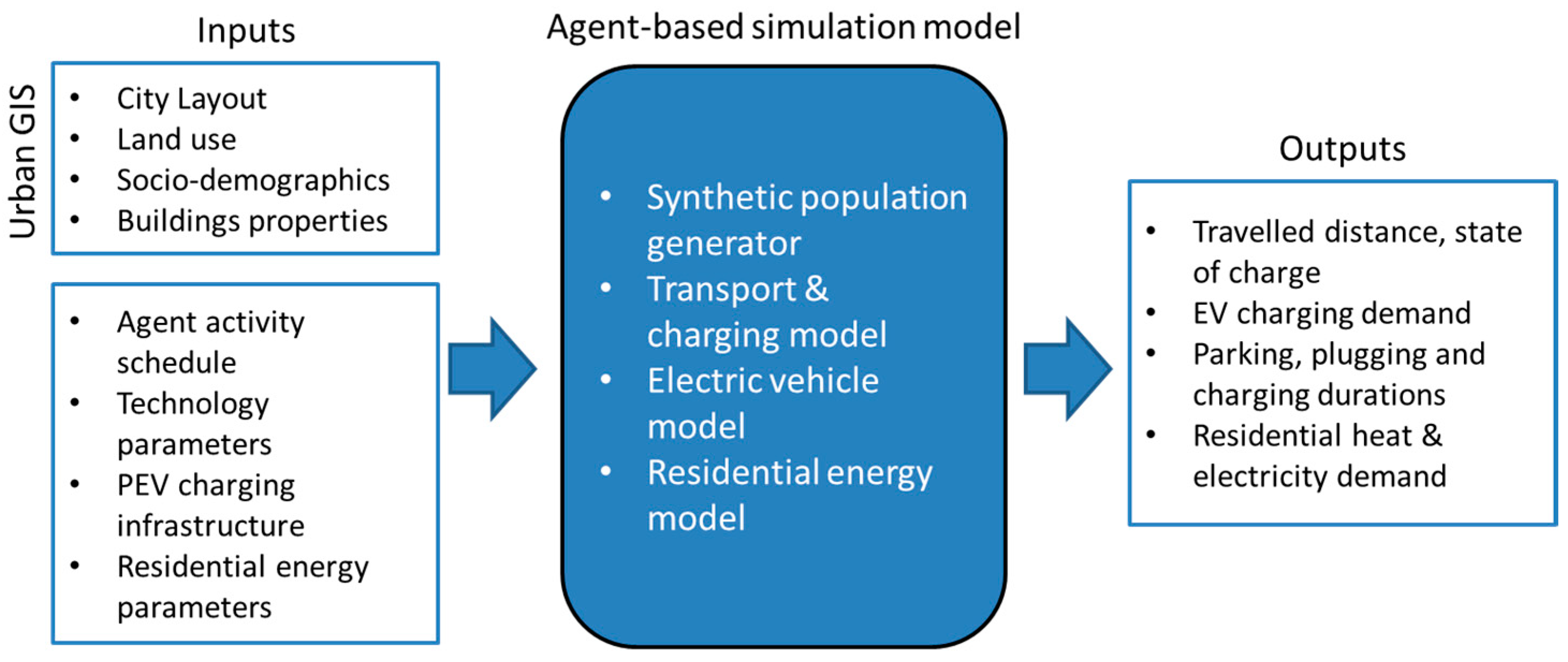
2. Materials and Methods
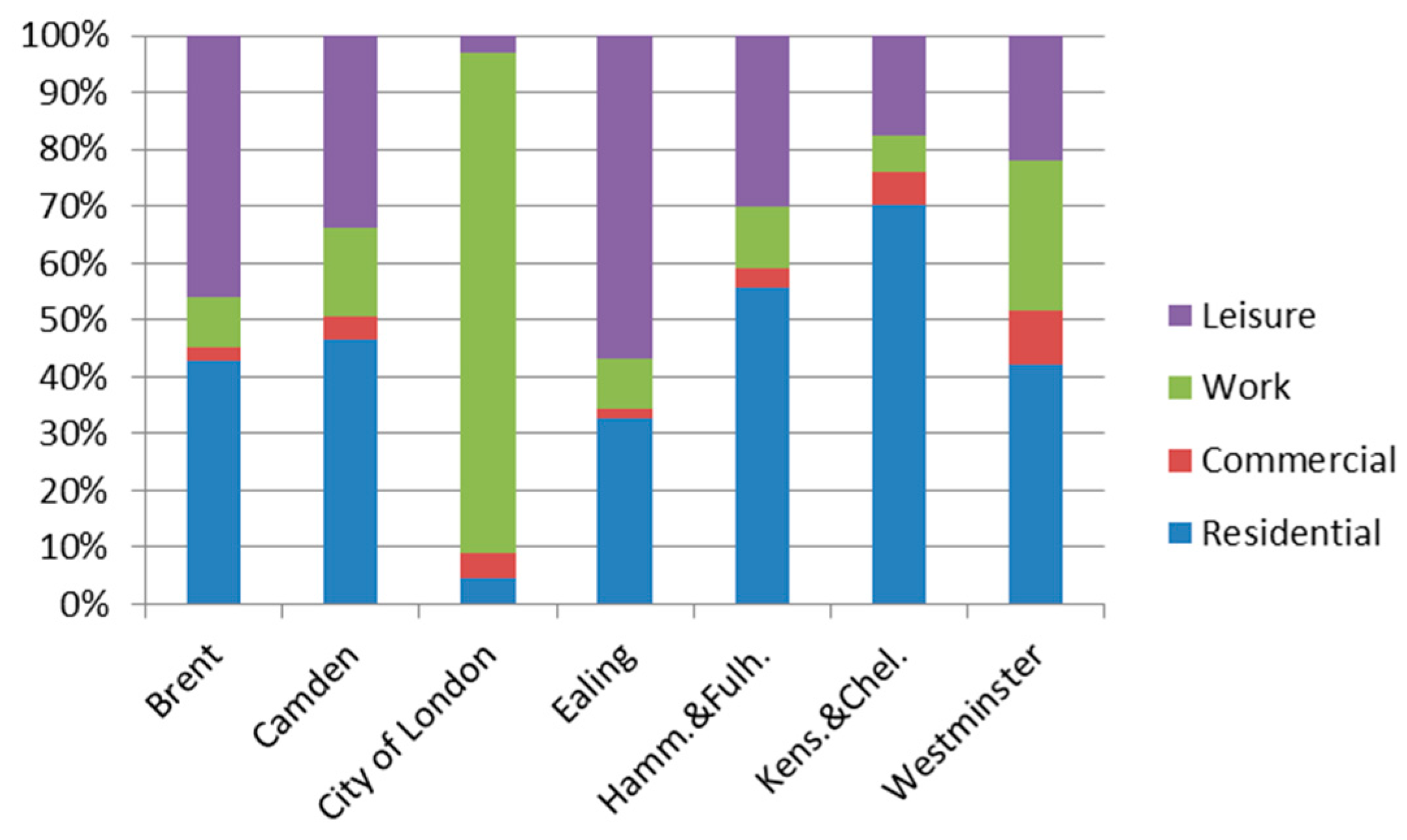
The framework presented in this work allows for the assessment of different scenarios related to transport and heat electrification in urban areas. The framework, therefore, supports the generation of a synthetic population for a given urban land use and demographics to simulate the daily activities of energy users. Finally, it estimates transport and energy demands together with several related key performance indicators. The decision support framework is built using the ABMS method [40,41], in which each agent represents an energy user, characterised by an internal state and a set of behavioural rules that define its interaction with the environment, generating energy service (electricity, heat and transport) demands.
As shown in Figure 1, the framework generates stationary and mobile energy demand profiles related to the residential sector and the (privately owned) electric vehicle fleet, respectively. These profiles are generated with a bottom-up approach in which the individual activities of energy users are the main drivers for transport demand and building occupancy patterns. These, in turn, generate the final PEV charging and building energy demands when combined with the physical and environmental properties of the system. In the process, different influencing factors such as the city layout, land use distribution, socio-demographic characteristics of users, weather conditions, technical parameters, and the charging and transport networks, are considered. More details of the sub-models are presented in the next sub-sections.
The framework is implemented using the free and open-source Java library Repast Simphony [42] and is built on top of the RepastCity model [43]. The code of this tool, under the name of SmartCityModel, is currently hosted in a private repository [44], but access to the source code can be granted upon request by contacting the corresponding author.
The general structure of the SmartCityModel is shown in Figure 2, where the main inputs (e.g., city layout, land use, vehicle technology, charging infrastructure) and outputs (e.g., travelled distance, state of charge (SOC), residential heat and electricity demand) are depicted. In the next sections, a more detailed description of each of the modules (namely synthetic population generator, transport and charging model, electric vehicle model, and residential energy model) is presented, together with the urban GIS-based representation as the main external input.

2.1. Urban GIS

To incorporate the spatial elements of the urban environment in which agents behave, a GIS-based representation is considered. The first vector layer, made of polygons, represents geographical areas (buildings, districts, boroughs, etc.), where synthetic agents carry out their different activities (being at home, working, shopping, leisure, etc.). The land use (residential, commercial, etc.), socio-demographic parameters (households, employment rate, vehicles), and building properties (heat loss parameter, height, etc.) can be defined for each spatial unit in this layer depending on the specific case study. A second vector layer is made of polylines to model the road network, which are defined by a set of links and nodes and represent streets and intersections, respectively. This allows agents to set routes and travel around the urban area between origins and destinations specified in the polygon layer. The distance travelled along this network is then used to estimate PEV energy consumption. When agents are not travelling, they occupy a specific spatial unit, generating the occupancy profiles that are then used in the static energy demand calculations. In this sense, the spatial resolution of the energy demand profiles will be determined by the scale of the spatial units.

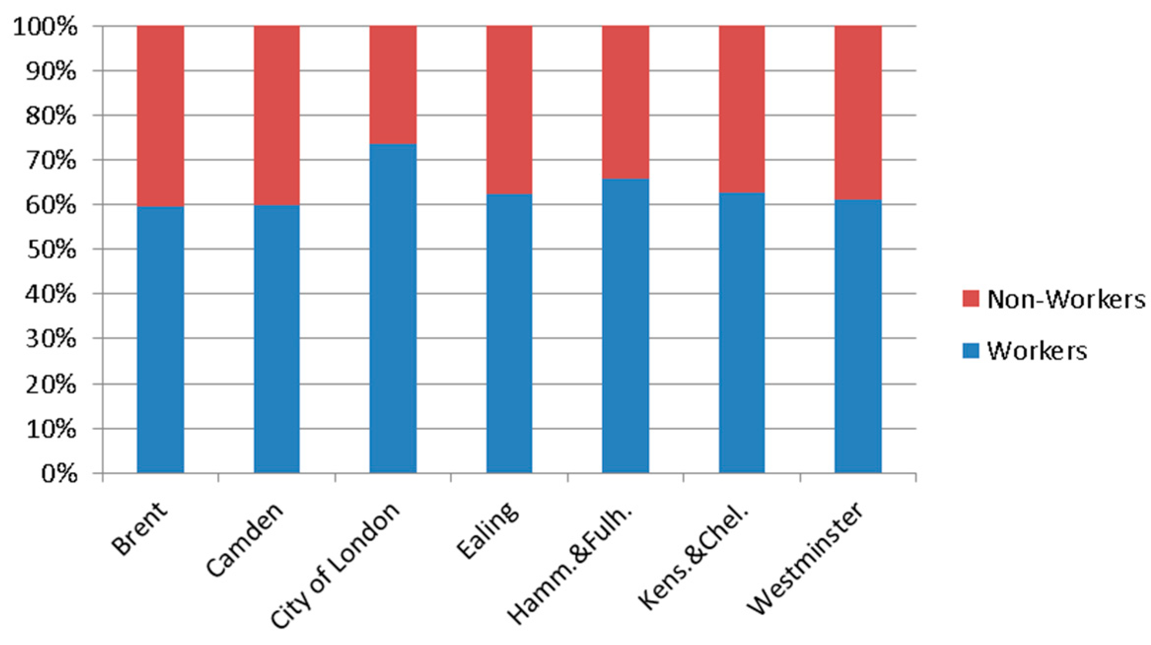
2.2. Synthetic Population Generator

The purpose of this module is to create a synthetic population of energy users living in the different zones of the urban area. This population, with their different activity schedules, will then generate energy demands that are spatially and temporally distributed throughout the city. Following the diagram shown in Figure 3, the first step is the creation of the environments based on the GIS model described previously, with each GIS layer representing a different aspect of the environment in which the agents behave (more information in [45]).
Once the environments are created, the next step is to generate a synthetic population of agents representing energy users. This process, implemented in the AgentFactory java class, creates the agents for each spatial unit, according to the attributes defined in the urban GIS model. Probability distributions are used extensively during the initialization of the model to define the agent’s properties, such as departure time, type of PEV (mini, small, medium), destination locations, etc., However, they are not used to inform the agent’s actions during the simulation, as these are driven by the agent’s decision rules. While the methodology was first introduced in [45], more details are incorporated in the current study. The steps to generate this synthetic population of energy users are the following. First, the number of agents p e v j in each spatial unit j is estimated based on the number of electric vehicles, which is dependent on the total number of vehicles v j and the general PEV adoption percentage α (see Equation (1)).
p e v j = v j × α ,
Then, the agent’s activity locations are defined by considering four different activities, each one related to a different land use (i.e., home with residential, workplace with work locations, shopping with commercial, and leisure activities with leisure areas). Then, for each agent, home and work locations are considered fixed and defined based on a probability proportional to the total floor space area (considering the height of buildings) linked with each activity (e.g., spatial units with higher proportions of residential/industrial floor space area will have higher numbers of agents living/working there).
Once an agent’s home and workplace are selected, its working status (worker, non-worker) is defined (note that a workplace is defined for all agents, including those with non-worker status, potentially accounting for agents looking for jobs or visiting offices). This definition uses the employment rates for each spatial unit, defined previously in the GIS model. Next, the PEV charging access level (defined as the probability for an agent to have a charging point of a specific type available) is set for each location. Then, each agent is associated with a PEV with a specific set of properties (more details are presented in Section 3.1.4), including an initial state of charge ( S O C i n i ), based on whether the agents have access to a charging point at home, and its activity schedule, defined according to its employment status. Based on the methodology presented in [45], the activity schedule A S i is created for each energy user (agent i ) according to its type (workers, non-workers) and it is defined with a list of 4-tuples, as shown in Equation (2).
A S i = A C T a , M D T a ,   S D a , P D a   ,
In Equation (2), A C T a denotes the specific agent’s activity, with a representing its category (work, home, shopping, leisure). In this equation, the departure time is defined as a normally distributed random variable, with M D T a as its mean departure time (in hours) and S D a as its standard deviation (in hours) to account for variability in the departure time among agents. Finally, a probability of departure P D a is included to account for the fact that not all agents will perform the same activities (e.g., irregular shifts, non-worker agents going to an office in the morning, workers going shopping in a retail area at lunchtime, etc.). After the initialisation of the environment and the population, these schedules are then used in the transport and charging model to generate trips; further details are presented in the next section.

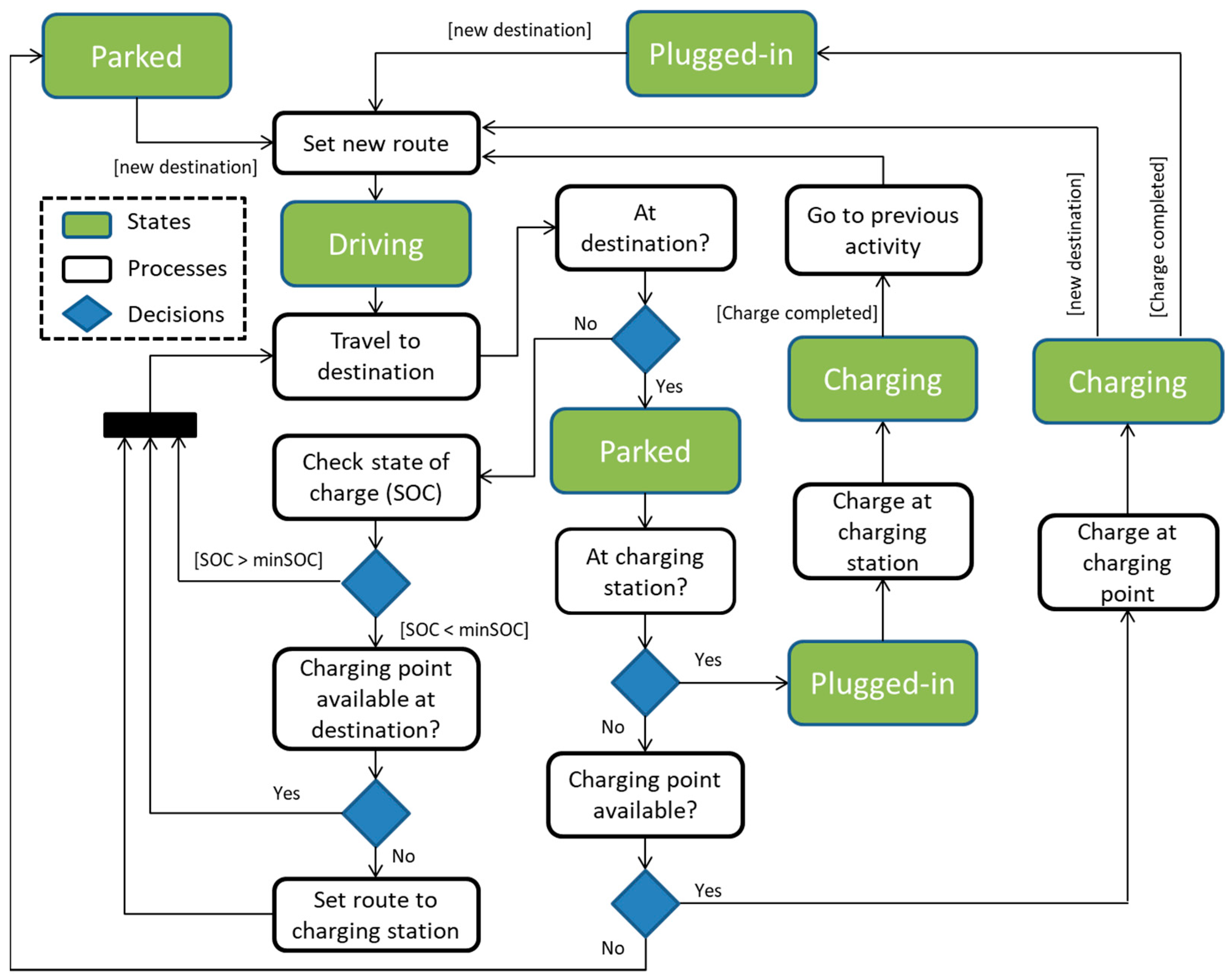
2.3. Transport and Charging Model

For the transport and charging model, trips are generated based on the agent’s activity schedules, defined previously in the synthetic population generation stage (see Equation (2)). Among other variables, each agent has a state variable that is used to keep track of the current state of the agent (parked, plugged, charging, or driving). During the time-driven simulation, agents will keep updating these variables as they perform their activities around the city, using the road network and occupying different buildings. Each agent will remain parked or plugged or charging (at a charging point) until a new activity is created (for simplification, it is assumed all agents are parked in their homes at the beginning of the simulation at 4 a.m.). When it is time for the next activity, the agent chooses their destination. For the case of home and work, the destination is fixed and defined previously in the synthetic population generation stage (see Section 2.2). In the case of shopping and leisure activities, their destinations are selected during the simulation before their starting time. The locations of these non-fixed destinations are set using the same allocation rule as in the case of home and work (i.e., based on a probability proportional to the specific floor space). Once the destination is defined, the route between the origin and destination is set based on the shortest path between the two sets of coordinates, and the agents start the new journey (changing their state variable to driving). Figure 4 shows the decision-making process considered for this first part of the simulation.
In this work, the charging decision model is formulated in terms of conditional logic rules. Although this proposed model generates realistic agent behaviour and is easy to implement, it is important to consider that there are many variations that could be implemented within the tool, depending on the specific case study. A review of different charging behaviours and location choice modelling is presented in [46]. Agents will keep travelling until their PEV’s state of charge (SOC) falls below a certain threshold (SOCmin), assuming the driver will have access to this information (the value of this parameter is scenario-specific). In this low battery condition, agents make the decision to charge (either at their destination or at a charging station) based on the availability of a charging point at their destination. If there is a charging point available at their destination, agents keep travelling and charge their PEV upon arrival (it is assumed the minimum state of charge would allow every agent to reach their destination). If there is no access to a charging point at their destination, agents set a new route to a public access charging station, changing their destinations temporally. It is worth noting here that there will be some cases where agents will need to travel more in order to find a public charging point. In this sense, there is an effect of the charging point location on the travelled distance, and, therefore, on the charging electricity demand. Upon arrival, agents will charge until the SOC reaches a maximum value SOCmax. After the charge is completed, agents continue to travel to their original destination before going to the charging station. Once they arrive at their destination, they check if there is a charging point available (independent of the SOC). If so, they will start charging their PEV until either the battery is fully charged (in which case it will remain plugged in), or the next activity starts. The previous process is then repeated for all agents for each time step until the end of the simulation. The travelling and charging behavioural model described previously is summarised in the activity diagram shown in Figure 5.

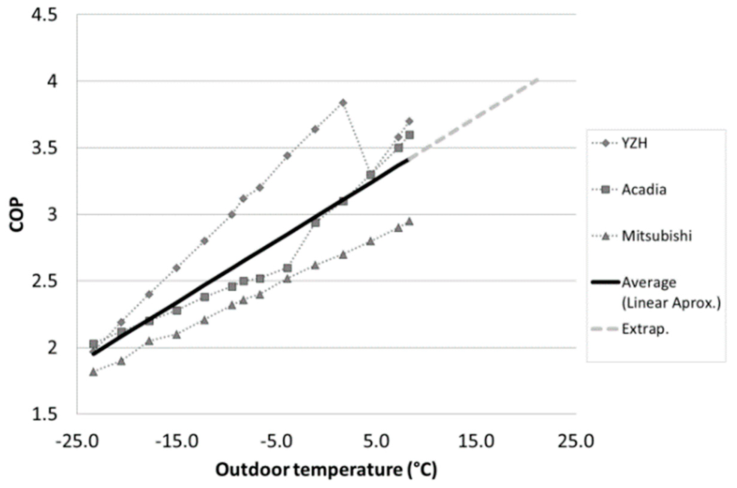
2.4. Plug-In Electric Vehicle Model

Plug-in electric vehicles are modelled as a generic energy storage device with the following properties: battery capacity, energy consumption rate, and round-trip efficiency. When PEVs are charging, power flows from the grid to the PEV battery, and the s o c i , t % (in terms of the percentage of battery capacity) is calculated at each time using Equation (3). For simplicity, the effect of the round-trip efficiency is considered only during the charging process.
s o c i , t + 1 % = 1 b a t t C a p i s o c i , t e + c h R a t e i × η 100 × t × 100 ,
In Equation (3), b a t t C a p i is the battery capacity (in kWh) of the PEV related to agent i , s o c i t e is the state of charge (in terms of absolute energy, in kWh) of agent i at time t , c h R a t e i is the charging power rate (in kW) of the charging point or charging station where agent i is currently charging, η is the round-trip efficiency that accounts for the losses in the charging and discharging processes, and t is the simulation time step.
For each time step, when the PEV is travelling to its destination, the PEV discharging process is characterised by Equation (4).
s o c i , t + 1 % = 1 b a t t C a p i s o c i , t e d i s t i , t × e R a t e i × 100 ,
where d i s t i t is the distance travelled by the agent (in km) during the time step and e R a t e i is the energy consumption rate (in kWh/km) of the vehicle related to agent i .

2.5. Residential Energy Model

The travel and charging behavioural rules previously described allow the simulation model to generate trips and charging events for the whole PEV fleet in the simulated urban area. These activities and trips create occupancy patterns for each of the spatial units defined in the city. These patterns are then used to generate electricity and heat demand profiles for residential areas using the following steps.
Residential occupancy r e s O c c j , t is calculated at each time step based on the number of awake residents r e s A w a k e j , t and the total inhabitants i n h a b j for each spatial unit j (see Equation (5)).
r e s O c c j , t = r e s A w a k e j , t i n h a b j ,
The residential electricity demand r e d j , t (in kW) for each spatial unit j and simulation time step t is generated using Equation (6) considering a base ( L b a s e j ) and a peak ( L p e a k j ) load (both in kW), the number of households per spatial unit ( H H j ) and the residential occupancy profile generated previously. This electricity demand does not consider the extra electricity demand from PEVs and HPs.
r e d j , t = H H j · L b a s e j + L p e a k j L b a s e j × r e s O c c j , t ,
The residential space heating demand r h d j , t (in kW) for each spatial unit j and simulation time step t is generated using Equation (7) considering the difference between indoor ( T i n j , t ) and outdoor ( T o u t t ) temperatures (both in K), the heat loss parameter H L P j (in W/m2K), the residential floor area R F A j (in m2), and the occupancy profile generated previously. This approach is similar to the traditional heating degree day method, but hourly data is used instead, and the occupancy of the whole zone is included in the calculation.
r h d j , t = T i n j , t T o u t t × H L P j × R F A j × r e s O c c j , t ,
The residential heat pump electricity demand r h p d j , t (in kW) is estimated for each spatial unit j and simulation time step t using Equation (8), where C O P t is the coefficient of performance (dimensionless), r h d j , t is the residential heat demand, and H P A L j is the adoption level (in %) of heat pumps for each spatial unit.
r h p d j , t = H P A L j × r h d j , t / C O P t ,
The C O P t is calculated for each time step depending on the external temperature. This effect is estimated based on the results presented by Caneta Research Inc. (North York, ON, Canada) [47] for a set of commercial air-source heat pumps, as shown in Figure 6.
The linear approximation shown in Figure 6 is used to characterise the effect of outdoor temperature T e x t t (in C) on the C O P t , according to Equation (9).
C O P t = 0.04627 · T e x t t + 3.03283 ,

3. Results

To demonstrate how the model can be used to provide decision support to key stakeholders, this section shows a detailed case study that applies this methodology to an urban area within London, UK. The model inputs and main assumptions are described with a general description of the results generated.

3.1. Model Inputs and Assumptions

In the next sub-sections, the main inputs and assumptions used in the SmartCityModel tool are described.

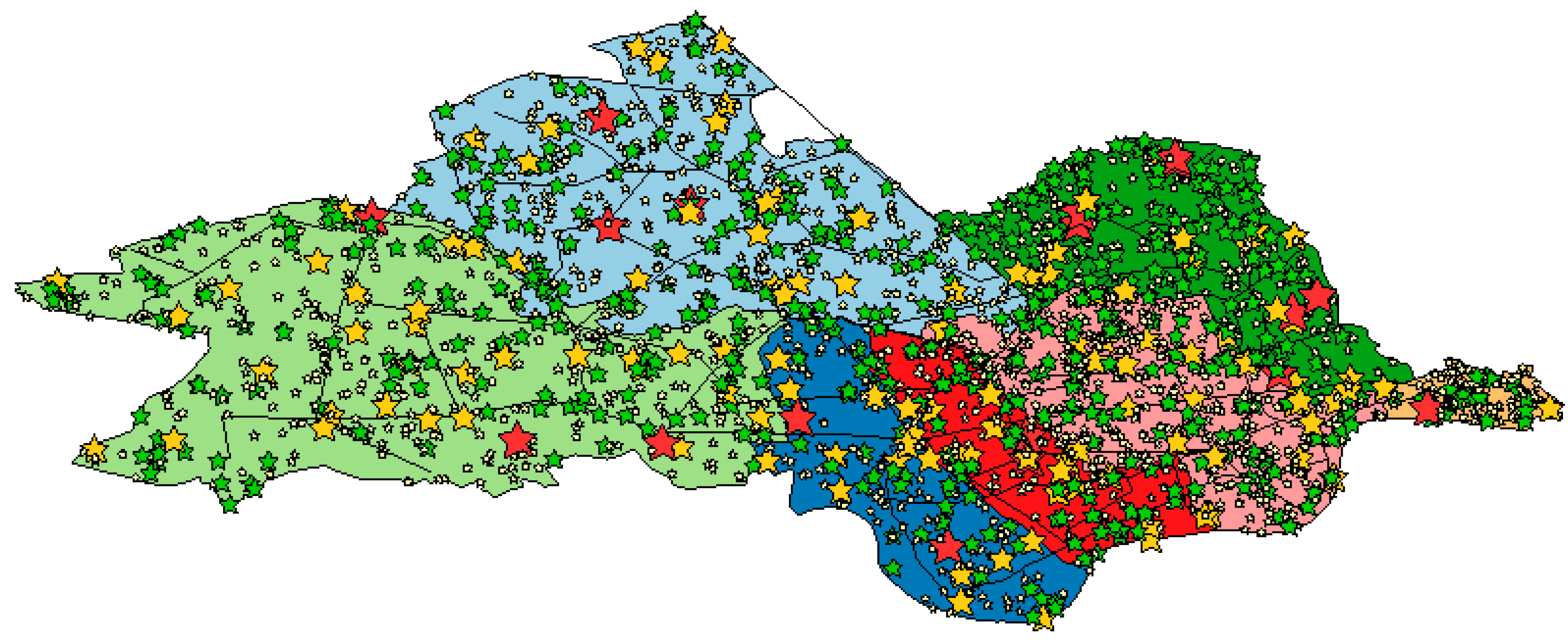
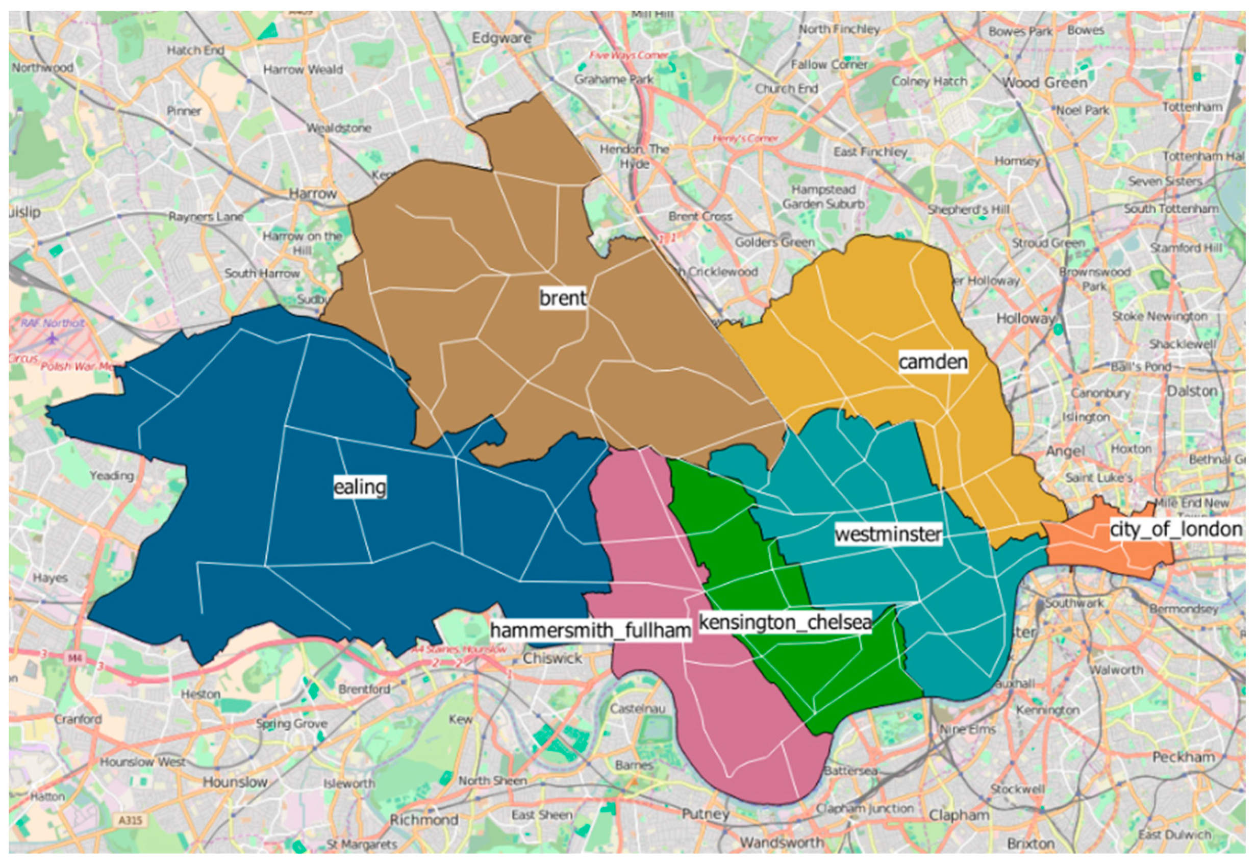
3.1.1. GIS City Model

The urban area under study is shown in Figure 7. It includes seven boroughs in central and west London, with a total area covering approximately 176 km2 and a total population of 1.4 million [49]. Geographic information system (GIS) data were used in the definition of the spatial units and the transport network. Data for the road network were extracted from the Ordnance Survey [50] and, for simplicity, they consider only the main roads. The urban area is considered closed; therefore, trips from/to external areas are not represented in this case study.
In this case study, each of the spatial units represents a borough with its specific socio-demographic information (number of households, vehicle ownership, employment rate, and land use) extracted from census data [49]. To estimate the employment rate, the population is classified into two groups: workers and non-workers. Based on the categories used in [49], the worker group is defined as including all the economically active employees and self-employed, while the non-workers group includes economically active unemployed, students, and other economically inactive populations (e.g., old age pensioners). The distribution of these groups is shown in Figure 8.
The land use distribution is simplified into four different types, namely residential, commercial, work, and leisure, which are linked to the agent activities according to the activity allocation criteria explained in Section 2.2. For each of these types, the floor area is estimated using the Land Use Statistics and Commercial and Industrial Floorspace information from the Office for National Statistics (ONS) [49], which is aggregated in Table 1.
In the case of the residential floor area, this information is not directly available (only land use is provided) and, therefore, it is estimated using the average floor area for all the properties in each borough, extracted from [51], and multiplying it by the number of households, extracted from census data. The final land use distribution is shown in Figure 9.

3.1.2. PEV Ownership and Technology

The estimation of the number of electric vehicles in the simulation is based on the level of PEV adoption (which is scenario-specific) and the car ownership for each borough [49], assuming PEVs will follow the current vehicle ownership distribution. In this work, the total number of PEVs is disaggregated among different PEV types (including plug-in hybrid electric vehicles, battery electric vehicles, and extended-range electric vehicles) to account for the heterogeneity in PEV technical parameters, such as battery capacity and energy consumption rate. Following the methodology presented in [52], the parameters and the market share used for this specific case study are presented in Table 2. The average speed is assumed to be constant and equal to 40 kmph based on a mobility survey [53], and the round-trip efficiency is assumed to be 90% (considering battery and charger).

3.1.3. PEV Charging Infrastructure

Access to charging infrastructure is determined depending on the location type (home, work, and public areas) and single probabilities. Using information from Zap-Map’s EV Charging Survey [54], it is assumed that 83% of EV users have access to a charging point at home, and 16% have access at work, in both cases with 7 kW as the most common charging power rating. For public charging points, using data from Zap-Map [55], it can be estimated that 13,378 connectors have been installed by 2021, with most of them being “fast”. It is also shown that most users prefer to use the 7 kW fast-charging option. Also, according to DfT and DVLA [56], London has a current fleet of 53,413 plug-in electric vehicles. With these figures, it can be estimated there is approximately one charger for every four PEVs; therefore, a 25% probability of access with a charging rate of 7 kW is assumed for the simulations. Finally, to account for the cases in which the PEV is running out of battery, a “Rapid” public charging station is considered in each borough, and for simplicity, it is located at the centroid of the spatial unit with a charging rate of 50 kW. In this case study, it is also assumed a total interoperability between different vehicles and chargers, so there are no additional access restrictions.

3.1.4. User Activities and PEV Charging Behaviour

The activity schedule for each agent is created based on the statistical definition given in Section 2.2. For this case study, an example of a general weekday schedule is considered, depending on the agent’s economic activity (i.e., worker or non-worker). The activity schedules are shown in Table 3 (see Equation (2) in Section 2.2. for details), and the parameters used for the PEV charging model, described in Section 2.3, are presented in Table 4. These are defined arbitrarily to include more heterogeneity in EV charging events. For example, an 80% battery charge is considered for public charging points, assuming users will prefer to reduce their charging time during their daily activities, preferring to fully charge when they are at home.

3.1.5. Residential Energy Demand Parameters

The parameters used in the residential electricity demand model (see Section 2.5) are estimated using the “Domestic Unrestricted” load profile from [57]. The values are presented in Table 5. For the heat loss parameter, the average for the UK (3.2 W/m2K) was considered [58]. An average temperature profile is used to represent different seasons (summer and winter) based on hourly data available in Met Office [59] for a weather station located in Heathrow, London, for 2014. Finally, an internal comfort temperature of 20 °C is used for all spatial units (boroughs) and the whole simulation (24 h). For this particular case study, a 10% adoption of residential heat pumps is considered.

3.2. Model Results

After the definition of the case study, the model is implemented and run to simulate a 24 h period with a time step of 5 min, starting at 4:00 a.m. on a weekday. A snapshot of the simulation is shown in Figure 10, where each star denotes an individual PEV, with its size and colour representing the SOC level (big and red for a low SOC, medium size and yellow for a medium SOC, and small and green for a high SOC). In the next sections, different results are shown to highlight the potential of the SmartCityModel tool to generate and evaluate different scenarios of transport and heat electrification in urban areas.

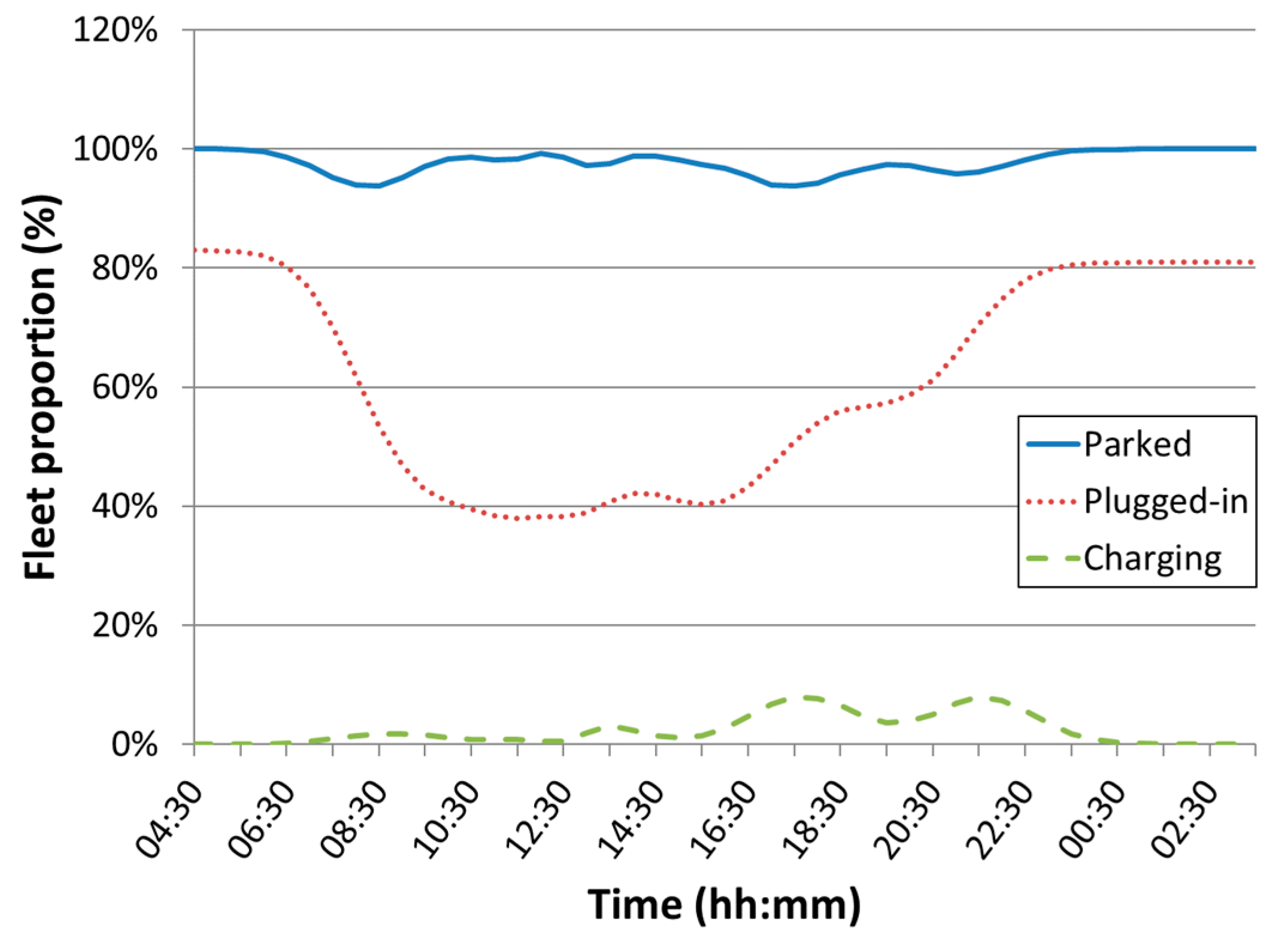
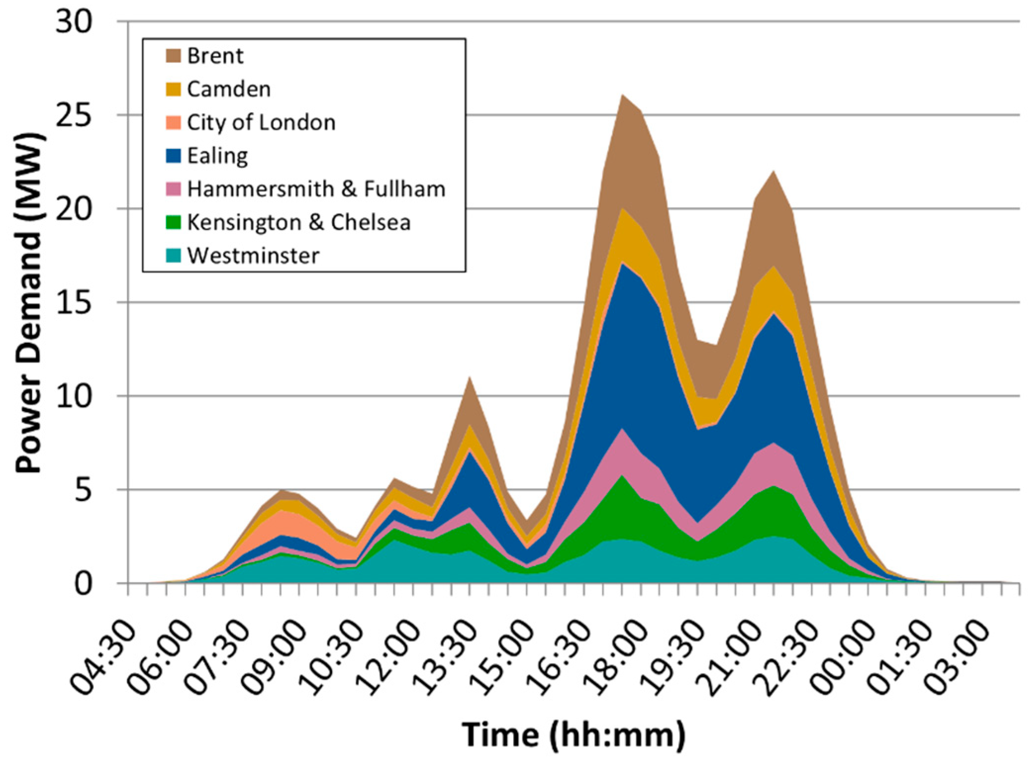
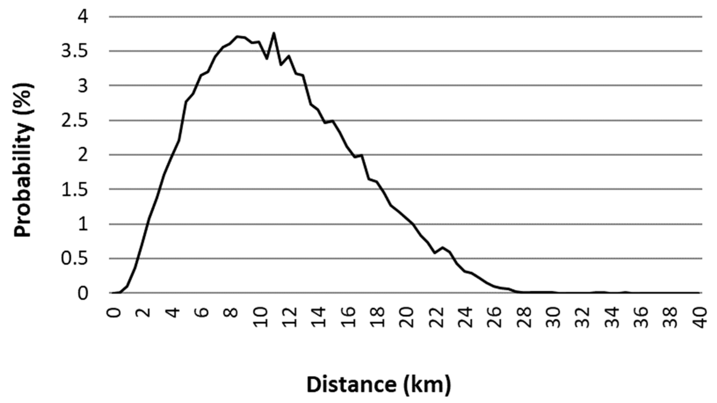
3.2.1. Travel and Charging Demand

For this part of the analysis, a scenario with 10% PEV adoption is considered, representing a fleet of 38,611 vehicles. Based on simulation results, the transport demand can be characterised by the probability density (Figure 11) and the cumulative distribution (Figure 12) functions to show the variation in trip distances for the whole PEV fleet during a day.
Figure 11 and Figure 12 show similar shapes compared to the results from trials and surveys found in the literature [60,61]. However, without specific data for London, a more comprehensive validation is hard to perform, as the results vary considerably from region to region. Nevertheless, Table 6 shows some relevant transport demand indicators that can be compared with statistics for England [62] and London [63], indicating that simulation results are within the range of realistic values. The difference observed in the average distance per trip, where simulation results show a higher value, especially when contrasted with London’s statistical data, can be explained by the distribution of land use across each borough and the delineation of the urban area. In the context of this case study, central London is located in the eastern periphery of the urban area (see Figure 7) and, as the borough with the highest proportion of work-related land use (see Figure 9), it attracts a higher proportion of trips related to work activities compared to what would be anticipated in a real-world scenario.
In terms of charging behaviour, Figure 13 shows the temporal variation in the proportion of the PEV fleet that is parked, plugged in, or charging (i.e., whenever the vehicle is not driving). In the case of parking proportion, the results of the simulation show that on average, 97.7% of the fleet is parked at any time of the day. This value is very similar to those found in the literature, in which it is suggested that an average vehicle is parked 96.5% of the time [64]. However, the proportion of plugged and charging vehicles is much lower. According to the simulation results, 60.7% of the fleet is plugged in and only 2.7% is charging on average during the day. These results are relevant to assess the level of flexibility PEV fleets can offer to charging management strategies that take advantage of the best time in the day (e.g., lower charging price, lower emissions) to charge the PEVs. In this sense, these strategies will be constrained by the number of PEVs that are plugged in and/or charging at different times and locations throughout the urban area.
The charging of PEVs generates an electricity demand in different zones (i.e., boroughs) of the urban area. Figure 14 shows the aggregated charging profiles of the whole PEV fleet for the different boroughs considered in the case study.
Results of the simulation show how the charging demand varies temporally and spatially depending on the land use, agents’ activity schedules, and level of access to charging infrastructure. For example, boroughs with high levels of workplace land use (e.g., the City of London, Westminster) present an important PEV charging demand during the peak hours in the mornings, which are associated with agents who can charge their PEV at work. A different result is obtained for boroughs with high residential and leisure areas (e.g., Ealing, Brent, Kensington, and Chelsea), where the charging demand is focused on the evenings when drivers charge their vehicles after arriving at home.

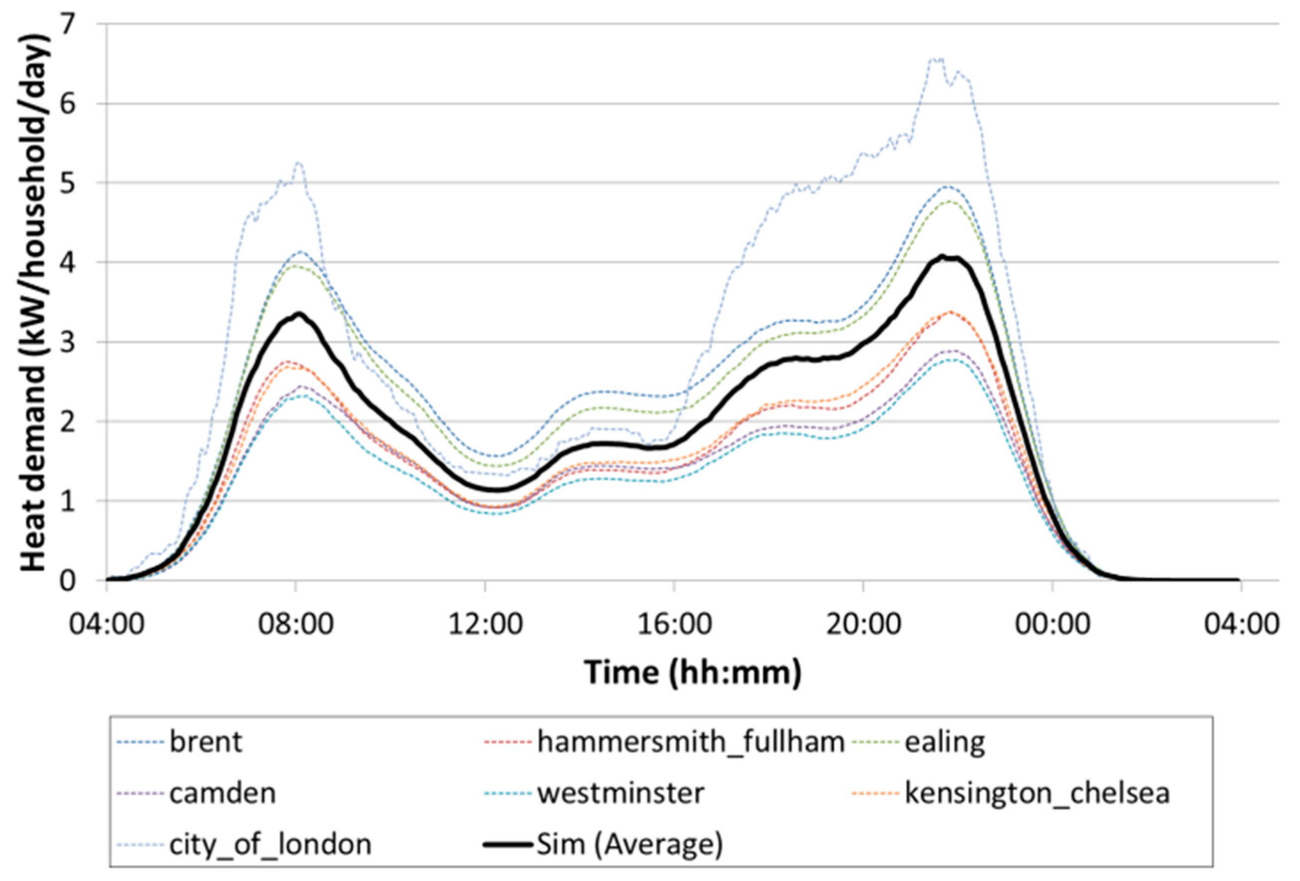
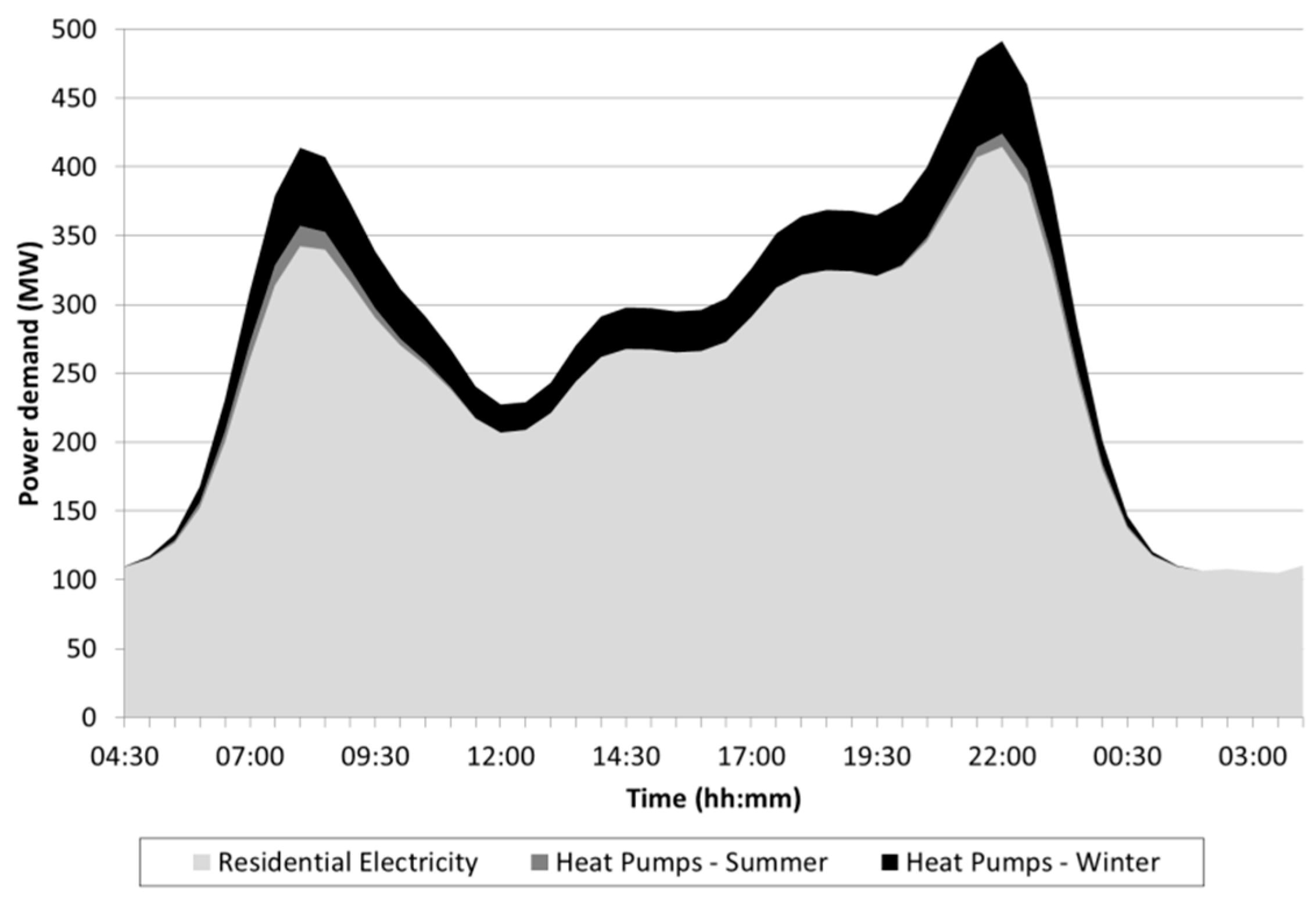
3.2.2. Residential Energy Demand

Some of the results shown in this section were first published in [62] and here they are shown, for completeness, as examples of outputs that can be generated by the tool. Figure 15 and Figure 16 show, for each borough, the residential daily electricity and heat demand profiles, respectively. The similitude in the shape of these curves is expected, as occupancy is one of the main influencing factors of energy demand in buildings. Depending on the specific situation, this assumption could be challenged. For example, in periods of partial occupancy, it can underestimate the real demand, as there could be cases where occupants use the heating system at full capacity or turn on the lights (or any other electrical appliance) without fully occupying the property, or even keep the heating system running (or the lights on) when nobody is at home.
The effect of the outdoor temperature on the heat demand can be seen in Figure 17, where heat profiles are compared for two different seasons (summer and winter). It is important to note these temperature profiles represent the three-month average for each season (winter and summer) and, therefore, the variability of the temperatures is smoothed.
In Figure 18, PEV charging demand is added on top of the residential demand for various levels of PEV adoption (from 10% to 50%). This figure represents the total residential electricity demand of the whole urban area, while similar graphs could also be generated for individual areas.
The results show that the additional electricity demand for PEV charging could represent an important proportion of the residential demand in certain periods. For example, for a 10% adoption level, the additional demand represents just 2% (on average) of the residential load, with a maximum of 6% around 18:00. For a 50% adoption, PEV demand represents 11% of residential demand (on average), with a peak of 29% at around the same time.
Finally, Figure 19 shows the electricity demand associated with the use of heat pumps when considering a 10% adoption of this technology in residential buildings.
The simulations show that the impacts will have a seasonal dependence, with winter being the most critical period of the year. Although, in summer, this demand can represent up to 5%, and during winter peak times it can represent up to 17% of the baseline residential electricity demand.

4. Discussion and Other Case Studies

The simulation framework presented in this work has been developed iteratively, sometimes in different directions, to increase its capability of supporting the evaluation of a diverse set of prospective scenarios, interventions, and strategies. More than 10 case studies (see Table 7) have been developed using the SmartCityModel tool alone or in combination with other models. For example, when evaluating different urban designs, the tool can be used to simulate the impact of different urban layouts and land uses on mobility patterns and their respective energy requirements. On the other hand, when looking at strategies to reduce the impact of electrification of transport and heat on the existing electricity infrastructure, the simulation tool, combined with optimization models, can help in the evaluation of different energy management mechanisms. Finally, behavioural aspects of energy users can be included in the analysis to evaluate the effectiveness of measures to incentivise changes in user habits such as flexible thermostat set points, PEV charge shifting, etc. Due to the variety of aspects to be covered by the proposed framework, the development of the simulation tool has been performed in a collaborative way, making use of open-source libraries and a shared platform to keep track of different versions of the main code. Table 7 summarises a selection of case studies that have been implemented during the last decade, using and extending the presented SmartCityModel tool. This table showcases the flexibility and modularity of the framework, as well as an indication of the size of the user base. By providing different (spatial) input data, new case studies were set up and extensions and modifications were made, where applicable, to include different sets of behaviours (e.g., taxi drivers rather than personal transport or non-residential buildings rather than domestic), which could then be utilised in future applications of the framework.
Table 7 shows all the applications where the proposed framework has been used/extended, supporting the notion of this framework being extensible and applicable to other geographies, user types, etc.
As mentioned in the literature review, the tool developed in this work aims to fill some important gaps related to the integrated planning of future urban energy systems. However, some challenges remain with respect to the integrated simulation of transport and building energy demands. In the current version, the tool is able to simulate only private vehicles with domestic users, with no consideration of public transport or commercial fleets (although taxis have been included in [67,70], and a simplified version of the commercial fleet in [66]). Similarly, most case studies consider only residential buildings. Commercial, industrial, and public buildings have only been considered in a simplified way in [68], as their energy demand characterization is more challenging. In these types of buildings, the electricity and thermal demands are not necessarily dependent on an hourly occupancy profile, and their energy intensity is strongly dependent on the specific purpose of the building. Finally, the current building thermal model accounts only for residential space heating, without considering hot water or any other process heat demand.
Another limitation of the tool is the fact it has been mainly tested in small and medium-size urban areas (except for the case studies presented in [67,72]). We expect that some of the behavioural rules of the agents might not be realistic when considering very large scenarios, especially those related to the choice of locations for different activities (work, shopping, leisure, etc.). However, the framework presented can easily be adapted to those scenarios by updating the initialization or behavioural rules implemented for the agents, or by providing new input data. The modular and extensible nature of the framework, as demonstrated by the varied use cases, shows that the approach can be modified when required, and different types of agents and activities could be added.
Finally, the proposed modelling framework has not gone through a rigorous and complete validation process. The complexity of the represented system and the lack of real-world data make it considerably hard to validate such a model. In order to assess if the results are sensible, we have attempted to partially validate the framework, comparing some of the results with aggregated (temporally and/or spatially) information. For example, the comparison shown in Table 6 (see Section 3.2.1) is used only to check if the simulation results were in the order of magnitude of real data (sanity check), as a full validation of travel demand would need a careful examination to make sure the real data represent a similar system to the simulated one (similar urban boundaries, user types, etc.). Another example of the partial validation of the modelling framework is presented in [48], where simulation results are compared to statistical data on residential annual electricity and heat demand for an urban area in London at the borough level.

5. Conclusions

The agent-based simulation model developed and presented in this work allows for a unified analysis of transport and building electrification. The modelling framework allows for the representation of a heterogeneous group of energy system users, each one with their own specific energy requirements as a result of their individual behaviour, interacting with the rest of the built environment and relevant energy systems for transport, heating, and power. Taking this generative and bottom-up modelling approach, spatiotemporal energy demand profiles can be produced and analysed for a spatially explicit urban area under various behaviour scenarios and linked directly to land-use distributions and urban planning settings.
A case study was presented to show the potential of the framework to analyse the impact of the additional electricity demand from both transport and building electrification in an integrated fashion. This case study was based on a future scenario where the private residential transport and heat demand is partially electrified. This study focused on understanding the energy requirements related to the charging of electric vehicles and the use of heat pumps in residential buildings. The results of this application showed that the model can generate realistic transport behaviour, which is necessary to estimate the charging and energy requirements as well as the utilization of the charging infrastructure. It was also shown that the simulation model is a useful tool to estimate daily energy profiles for charging, power, and heat demand in different zones of the city and explore the influence of land use and agents’ activities and preferences on these demands.
Although it is still in an early stage, the modelling framework presented in this work can be used to estimate the impact of transport and heat electrification on current system load under different prospective scenarios and energy system pathways. While this study has provided valuable insights, it is important to acknowledge its limitations, as discussed in the previous section. These limitations pave the way for avenues of future work. In the context of transport systems, other transport agents, such as public transport and commercial fleets, can be incorporated, while also considering multimodal transport in which agents can switch between transport networks. Regarding heating demand, future versions of the tool should incorporate residential hot water demand, and the rest of the building sector (commercial, industrial, public) could also be considered. The presented framework can also be used to explore energy management strategies for PEVs and HPs, especially in electricity networks that would otherwise need to be upgraded to cope with the additional demand. Also, through a rigorous sensitivity analysis, the influence of each factor affecting the additional electricity demand could be assessed. Additionally, uncertainty analyses could be performed in future work, running multiple simulations considering the value of some parameters from specified ranges or probability distributions (modifying random number generator seed values). We are especially keen to explore how the framework will be used and extended by new users independently from the core team and monitor how the urban planning and urban modelling community can utilise the presented tools in helping to solve real and urgent global challenges.
To conclude, the agent-based modelling framework presented in this paper can be applied in a wide range of urban planning, transport, and energy management scenarios at the planning and operational levels. The outputs generated by the model can provide insights for planners, engineers, policymakers, network operators, etc., who are interested in the design and implementation of low-carbon solutions in urban areas. The applicability, flexibility, and extensibility of the model were demonstrated through a range of case studies, showing how the model can be initialised from spatial input data and have some elements configured without having to modify the source code, while the open-source nature of the SmartCityModel enables modellers to extend and adapt the tool where required. The framework will thus continue to provide relevant insights into the future of cities as part of the urgent transition to more sustainable urban environments.

Author Contributions

Conceptualization, G.B.-T., K.H.v.D., S.A. and N.S.; methodology, G.B.-T., K.H.v.D., S.A. and N.S.; software, G.B.-T., K.H.v.D. and S.A.; validation, G.B.-T., K.H.v.D. and S.A.; formal analysis, G.B.-T., K.H.v.D., S.A. and N.S.; investigation, G.B.-T., K.H.v.D., S.A. and N.S.; resources, G.B.-T., K.H.v.D., S.A. and N.S.; data curation, G.B.-T., K.H.v.D. and S.A.; writing—original draft preparation, G.B.-T., K.H.v.D. and S.A.; writing—review and editing, G.B.-T., K.H.v.D., S.A. and N.S.; visualization, G.B.-T.; supervision, K.H.v.D., S.A. and N.S.; project administration, K.H.v.D., S.A. and N.S.; funding acquisition, G.B.-T., K.H.v.D., S.A. and N.S. All authors have read and agreed to the published version of the manuscript.

Funding

The authors acknowledge financial support from the Chilean ANID-Fondecyt Postdoctoral Grant (project No. 3210460) and the Research Councils UK’s Digital Economy Programme (EPSRC grant No. EP/I038837/1).

Data Availability Statement

For the main case study (Section 3), the input data is publicly available (refer to respective references). The output data the model can be generated using the source code, currently hosted in a private repository [44]. Access to the source code can be granted upon request by contacting the corresponding author. As for the remaining case studies presented in Section 4, information regarding data availability can be found in their references.

Conflicts of Interest

The authors declare no conflict of interest. The funders had no role in the design of the study; in the collection, analyses, or interpretation of data; in the writing of the manuscript; or in the decision to publish the results.

Abbreviations

The next table shows the list of acronyms used throughout the article, with their respective units (where applicable).
AcronymDefinition
ABMAgent-based modelling
ABMSAgent-based modelling and simulation
CO2-eqCarbon dioxide equivalent
COPCoefficient of performance
DSMDemand-side management
EVElectric vehicle
GISGeographic information system
HPHeat pump
ONSOffice for National Statistics
PEVPlug-in electric vehicle
PHEVPlug-in hybrid electric vehicle
SOCState of charge
ToUTime of use

References

  1. United Nations. World Urbanization Prospects 2018, Highlights; Department of Economic and Social Affairs, Population Division; United Nations: New York, NY, USA, 2019. [Google Scholar]
  2. International Energy Agency (IEA). Empowering Cities for a Net Zero Future: Unlocking Resilient, Smart, Sustainable Urban Energy Systems; International Energy Agency (IEA): Paris, France, 2021. [Google Scholar]
  3. Ripple, W.J.; Wolf, C.; Gregg, J.W.; Levin, K.; Rockström, J.; Newsome, T.M.; Betts, M.G.; Huq, S.; Law, B.E.; Kemp, L.; et al. World scientists’ warning of a climate emergency 2022. Bioscience 2022, 72, 894–898. [Google Scholar]
  4. Rising, J.; Tedesco, M.; Piontek, F.; Stainforth, D.A. The missing risks of climate change. Nature 2022, 610, 1149–1151. [Google Scholar]
  5. World Health Organization (WHO). Ambient (Outdoor) Air Pollution, Key Facts; World Health Organization (WHO): Geneva, Switzerland, 2018. Available online: https://www.who.int/news-room/fact-sheets/detail/ambient-(outdoor)-air-quality-and-health (accessed on 13 October 2021).
  6. World Health Organization (WHO). Ambient Air Pollution: A Global Assessment of Exposure and Burden of Disease; World Health Organization (WHO): Geneva, Switzerland, 2018.
  7. C40 & Arup. Climate Action in Megacities Version 2.0. 2014. Available online: https://www.arup.com/perspectives/publications/research/section/climate-action-in-megacities (accessed on 15 October 2021).
  8. International Energy Agency (IEA). Global Energy-Related CO2 Emissions by Sector; International Energy Agency (IEA): Paris, France, 2021; Available online: https://www.iea.org/data-and-statistics/charts/global-energy-related-co2-emissions-by-sector (accessed on 13 October 2021).
  9. Hawkins, T.R.; Gausen, O.M.; Strømman, A.H. Environmental impacts of hybrid and electric vehicles—A review. Int. J. Life Cycle Assess. 2012, 17, 997–1014. [Google Scholar]
  10. International Energy Agency (IEA). Global EV Outlook 2021; International Energy Agency (IEA): Paris, France, 2021. [Google Scholar]
  11. International Energy Agency (IEA). Tracking Clean Energy Progress 2017; International Energy Agency (IEA): Paris, France, 2017. [Google Scholar]
  12. Chaudry, M.; Abeysekera, M.; Hosseini, S.H.R.; Jenkins, N.; Wu, J. Uncertainties in decarbonising heat in the UK. Energy Policy 2015, 87, 623–640. [Google Scholar]
  13. Committee on Climate Change. Next Steps for UK Heat Policy; Committee on Climate Change: London, UK, 2016. [Google Scholar]
  14. Department of Energy and Climate Change. Heat Pumps in District Heating: Final Report; Department of Energy and Climate Change: London, UK, 2016. [Google Scholar]
  15. O’Dwyer, E.; Pan, I.; Acha, S.; Shah, N. Smart energy systems for sustainable smart cities: Current developments, trends and future directions. Appl. Energy 2019, 237, 581–597. [Google Scholar]
  16. Pohekar, S.D.; Ramachandran, M. Application of multi-criteria decision making to sustainable energy planning—A review. Renew. Sustain. Energy Rev. 2004, 8, 365–381. [Google Scholar]
  17. Wang, J.-J.; Jing, Y.-Y.; Zhang, C.-F.; Zhao, J.-H. Review on multi-criteria decision analysis aid in sustainable energy decision-making. Renew. Sustain. Energy Rev. 2009, 13, 2263–2278. [Google Scholar]
  18. García-Villalobos, J.; Zamora, I.; Knezović, K.; Marinelli, M. Multi-objective optimization control of plug-in electric vehicles in low voltage distribution networks. Appl. Energy 2016, 180, 155–168. [Google Scholar]
  19. Akmal, M.; Fox, B.; Morrow, J.D.; Littler, T. Impact of Heat Pump Load on Distribution Networks. IET Gener. Transm. Distrib. 2014, 8, 2065–2073. [Google Scholar]
  20. Siano, P. Demand response and smart grids—A survey. Renew. Sustain. Energy Rev. 2014, 30, 461–478. [Google Scholar]
  21. Strbac, G. Demand side management: Benefits and challenges. Energy Policy 2008, 36, 4419–4426. [Google Scholar]
  22. Lund, H.; Østergaard, P.A.; Connolly, D.; Mathiesen, B.V. Smart energy and smart energy systems. Energy 2017, 137, 556–565. [Google Scholar]
  23. Vayá, M.G.; Andersson, G. Centralized and decentralized approaches to smart charging of plug-in Vehicles. In Proceedings of the 2012 IEEE Power and Energy Society General Meeting, San Diego, CA, USA, 22–26 July 2012. [Google Scholar]
  24. García-Villalobos, J.; Zamora, I.; San Martín, J.; Asensio, F.; Aperribay, V. Plug-in electric vehicles in electric distribution networks: A review of smart charging approaches. Renew. Sustain. Energy Rev. 2014, 38, 717–731. [Google Scholar]
  25. Patteeuw, D.; Henze, G.P.; Helsen, L. Comparison of load shifting incentives for low-energy buildings with heat pumps to attain grid flexibility benefits. Appl. Energy 2016, 167, 80–92. [Google Scholar]
  26. Pfenninger, S.; Hawkes, A.; Keirstead, J. Energy systems modeling for twenty-first century energy challenges. Renew. Sustain. Energy Rev. 2014, 33, 74–86. [Google Scholar]
  27. Keirstead, J.; Jennings, M.; Sivakumar, A. A review of urban energy system models: Approaches, challenges and opportunities. Renew. Sustain. Energy Rev. 2012, 16, 3847–3866. [Google Scholar]
  28. Allegrini, J.; Orehounig, K.; Mavromatidis, G.; Ruesch, F.; Dorer, V.; Evins, R. A review of modelling approaches and tools for the simulation of district-scale energy systems. Renew. Sustain. Energy Rev. 2015, 52, 1391–1404. [Google Scholar]
  29. Wei, S.; Jones, R.; De Wilde, P. Driving factors for occupant-controlled space heating in residential buildings. Energy Build. 2014, 70, 36–44. [Google Scholar]
  30. Daina, N.; Sivakumar, A.; Polak, J.W. Modelling electric vehicles use: A survey on the methods. Renew. Sustain. Energy Rev. 2017, 68, 447–460. [Google Scholar]
  31. Azadfar, E.; Sreeram, V.; Harries, D. The investigation of the major factors influencing plug-in electric vehicle driving patterns and charging behaviour. Renew. Sustain. Energy Rev. 2015, 42, 1065–1076. [Google Scholar]
  32. Li, W.; Stanula, P.; Egede, P.; Kara, S.; Herrmann, C. Determining the main factors influencing the energy consumption of electric vehicles in the usage phase. Procedia CIRP 2016, 48, 352–357. [Google Scholar]
  33. Sola, A.; Corchero, C.; Salom, J.; Sanmarti, M. Multi-domain urban-scale energy modelling tools: A review. Sustain. Cities Soc. 2020, 54, 101872. [Google Scholar]
  34. Robinson, D.; Haldi, F.; Leroux, P.; Perez, D.; Rasheed, A.; Wilke, U. CitySim: Comprehensive micro-simulation of resource flows for sustainable urban planning. In Proceedings of the 11th International IBPSA Conference, Glasgow, Scotland, 27–30 July 2009; pp. 1083–1090. [Google Scholar]
  35. Bergerson, J.; Muehleisen, R.T.; Rodda, W.B.; Auld, J.A.; Guzowski, L.B.; Ozik, J.; Collier, N. Designing future cities: LakeSIM integrated design tool for assessing short and long term impacts of urban scale conceptual designs. ISOCARP Rev. 2015, 11. [Google Scholar]
  36. Chingcuanco, F.; Miller, E.J. A microsimulation model of urban energy use: Modelling residential space heating demand in ILUTE. Comput. Environ. Urban Syst. 2012, 36, 186–194. [Google Scholar] [CrossRef]
  37. Keirstead, J.; Samsatli, N.I.; Shah, N. SynCity: An Integrated Tool Kit for Urban Energy Systems Modeling. In Energy efficient cities: Assessment Tools and Benchmarking Practices; World Bank Publication: Washington, DC, USA, 2009. [Google Scholar]
  38. Ghauche, A. Integrated Transportation and Energy Activity-Based Model. Master’s Thesis, Massachusetts Institute of Technology, Cambridge, MA, USA, 2010. [Google Scholar]
  39. Bustos-Turu, G. Integrated modelling framework for the analysis of demand side management strategies in urban energy systems. Ph.D. Thesis, Imperial College London, London, UK, 2018. [Google Scholar]
  40. Macal, C.M. Everything you need to know about agent-based modelling and simulation. J. Simul. 2016, 10, 144–156. [Google Scholar]
  41. Van Dam, K.H.; Nikolic, I.; Lukszo, Z. Agent-Based Modelling of Socio-Technical Systems; Springer Science & Business Media: Dordrecth, The Netherlands, 2012. [Google Scholar]
  42. North, M.J.; Collier, N.T.; Ozik, J.; Tatara, E.R.; Macal, C.M.; Bragen, M.; Sydelko, P. Complex adaptive systems modeling with Repast Simphony. Complex Adapt. Syst. Model. 2013, 1, 1–26. [Google Scholar]
  43. Malleson, N. Repastcity. 2012. Available online: https://github.com/nickmalleson/repastcity (accessed on 1 April 2017).
  44. Van Dam, K.; Bustos-Turu, G. SmartCityModel, GitHub Repository [Online]. 2016. Available online: https://github.com/albertopolis/SmartCityModel (accessed on 1 May 2022).
  45. Van Dam, K.H.; Bustos-Turu, G.; Shah, N. A methodology for simulating synthetic populations for the analysis of socio-technical infrastructures. In Proceedings of the 11th Conference of the European Social Simulation Association (ESSA), Groningen, The Netherlands, 14–18 September 2015. [Google Scholar]
  46. Adenaw, L.; Lienkamp, M. Multi-Criteria, Co-Evolutionary Charging Behavior: An Agent-Based Simulation of Urban Electromobility. World Electr. Veh. J. 2021, 12, 18. [Google Scholar] [CrossRef]
  47. Caneta Research Inc. Heat Pump Characterization Study; Caneta Research Inc.: Mississauga, ON, Canada, 2010. [Google Scholar]
  48. Bustos-Turu, G.; van Dam, K.H.; Acha, S.; Markides, C.N.; and Shah, N. Simulating residential electricity and heat demand in urban areas using an agent-based modelling approach. In Proceedings of the 2016 IEEE International Energy Conference (ENERGYCON), Leuven, Belgium, 4–8 April 2016; pp. 1–6. [Google Scholar] [CrossRef]
  49. Office for National Statistics (ONS). 2016. Available online: https://www.ons.gov.uk/census (accessed on 1 February 2016).
  50. Ordnance Survey. 2016. Available online: https://www.ordnancesurvey.co.uk/ (accessed on 1 February 2016).
  51. Mayor of London. Average Floor Area by Borough. 2015. Available online: https://data.london.gov.uk/average-floor-area-by-borough/ (accessed on 1 February 2016).
  52. Bustos-Turu, G. Operational Impacts of the Charging Infrastructure in the Electric Vehicle Spatial and Temporal Energy Demand and Grid Services Provision: An Agent-Based Modelling and Simulation Approach. Master’s Thesis, Sustainable Energy Futures, Imperial College London, London, UK, 2013. [Google Scholar]
  53. Pasaoglu, G.; Fiorello, D.; Martino, A.; Scarcella, G.; Alemanno, A.; Zubaryeva, A.; Thiel, C. Driving and Parking Patterns of European Car Drivers—A Mobility Survey; European Commission, Joint Research Centre, Institute for Energy and Transport: European Union: Brussels, Belgium, 2012. [Google Scholar]
  54. Zap-Map 2020, Zap-Map EV Charging Survey, Key Findings 2020. Available online: https://www.zap-map.com/ev-charging-survey/ (accessed on 27 September 2021).
  55. Zap-Map 2021, EV Charging Stats 2021. Available online: https://www.zap-map.com/statistics/ (accessed on 17 September 2021).
  56. Department for Transport (DfT) and Driver and Vehicle Licensing Agency (DVLA). Vehicle Licensing Statistics. 2021. Available online: https://www.gov.uk/government/statistical-data-sets/all-vehicles-veh01 (accessed on 17 September 2021).
  57. Elexon. Profiling. 2015. Available online: https://www.elexon.co.uk/reference/technical-operations/profiling/ (accessed on 1 February 2016).
  58. Palmer, J.; Cooper, I. United Kingdom Housing Energy Fact File: 2013; Department of Energy & Climate Change (DECC): London, UK, 2014. [Google Scholar]
  59. Met Office. Met Office Integrated Data Archive System (MIDAS) Land and Marine Surface Stations Data (1853-current). 2016. Available online: http://catalogue.ceda.ac.uk/uuid/220a65615218d5c9cc9e4785a3234bd0 (accessed on 1 February 2016).
  60. Pearre, N.S.; Kempton, W.; Guensler, R.L.; Elango, V.V. Electric vehicles: How much range is required for a day’s driving? Transp. Res. Part C Emerg. Technol. 2011, 19, 1171–1184. [Google Scholar]
  61. Lin, Z.; Dong, J.; Liu, C.; Greene, D. Estimation of Energy Use by Plug-In Hybrid Electric Vehicles. Transp. Res. Rec. J. Transp. Res. Board 2012, 2287, 37–43. [Google Scholar]
  62. Department for Transport (DfT). National Travel Survey Statistics. 2020. Available online: https://www.gov.uk/government/collections/national-travel-survey-statistics (accessed on 20 September 2021).
  63. Transport for London (TfL). London Travel Demand Survey—Workbook 2019/2020. 2021. Available online: https://tfl.gov.uk/corporate/about-tfl/how-we-work/planning-for-the-future/consultations-and-surveys (accessed on 20 September 2021).
  64. Bates, J.; Leibling, D. Spaced Out: Perspectives on Parking Policy; RAC Foundation: London, UK, 2012. [Google Scholar]
  65. Yang, L.; Zhang, L.; Stettler, M.E.; Sukitpaneenit, M.; Xiao, D.; van Dam, K.H. Supporting an integrated transportation infrastructure and public space design: A coupled simulation method for evaluating traffic pollution and microclimate. Sustain. Cities Soc. 2020, 5, 101796. [Google Scholar]
  66. Chakrabarti, A.; Proeglhoef, R.; Bustos-Turu, G.; Lambert, R.; Mariaud, A.; Acha, S.; Markides, C.N.; Shah, N. Optimisation and analysis of system integration between electric vehicles and UK decentralised energy schemes. Energy 2019, 176, 805–815. [Google Scholar] [CrossRef]
  67. Lowans, C. Integrated Planning of Electric Taxi Charging Infrastructure. Master’s Thesis, Sustainable Energy Futures, Imperial College London, London, UK, 2017. [Google Scholar]
  68. Ladas, P. Simulating Heat and Electricity Demand in Urban Areas an Agent-Based Modelling Approach in Residential and Non-Residential Buildings. Master’s Thesis, Sustainable Energy Futures, Imperial College London, London, UK, 2016. [Google Scholar]
  69. Briola, M. Agent-Based Modelling of Residential Heat Demand in a District Heating Network: A Decision Support Tool for Queen Elizabeth Olympic Park Case Study. Master’s Thesis, Sustainable Energy Futures, Imperial College London, London, UK, 2016. [Google Scholar]
  70. Xin, W. Simulation and Characterisation of Charging Infrastructure of ULEV Taxis in London. Master’s Thesis, Sustainable Energy Futures, Imperial College London, London, UK, 2016. [Google Scholar]
  71. Clifford, M. Decision Support for the Evaluation of Sustainable Urban Masterplans. Master’s Thesis, Sustainable Energy Futures, Imperial College London, London, UK, 2015. [Google Scholar]
  72. Ferard, M. Sustainable Energy Systems in Islands and Cities: Potential for Mutual Learning. Master’s Thesis, Sustainable Energy Futures, Imperial College London, London, UK, 2015. [Google Scholar]
  73. Plessiez, P. Mitigating the Impacts of Electric Vehicles on the Electricity Network through the Use of Smart Charging Strategies. Master’s Thesis, Sustainable Energy Futures, Imperial College London, London, UK, 2015. [Google Scholar]
  74. Mallet, E. Attractiveness to Customers and Profitability of Smart Charging Schemes for Electric Vehicles. Master’s thesis, Sustainable Energy Futures, Imperial College London, London, UK, 2015. [Google Scholar]
  75. Bustos-Turu, G.; Van Dam, K.; Acha, S.; Shah, N. Estimating Plug-in Electric Vehicle Demand Flexibility through an Agent-Based Simulation Model. In Proceedings of the 5th IEEE PES Innovative Smart Grid Technologies (ISGT) European 2014 Conference, Istanbul, Turkey, 12–15 October 2014. [Google Scholar]
  76. Acha, S.; Van Dam, K.H.; Keirstead, J.; Shah, N. Integrated Modelling of Agent-Based Electric Vehicles into Optimal Power Flow Studies. In Proceedings of the 21st International Conference on Electricity Distribution, Frankfurt, Germany, 6–9 June 2011. [Google Scholar]
Figure 1. Agent-based modelling and simulation framework data flow.
Energies 16 06312 g001
Figure 2. Agent-based simulation model structure.
Energies 16 06312 g002
Figure 3. Synthetic population generation.
Energies 16 06312 g003
Figure 4. Activity diagram for the transport and charging model (Part a).
Energies 16 06312 g004
Figure 5. Activity diagram for the transport and charging model (Part b).
Energies 16 06312 g005
Figure 6. Effect of external temperature on the coefficient of performance (COP) of an air-source heat pump. © 2016 IEEE. Reprinted with permission from [48].
Energies 16 06312 g006
Figure 7. Urban area in West and Central London, UK. © 2016 IEEE. Reprinted with permission from [48].
Energies 16 06312 g007
Figure 8. Employment rate for each borough (Brent, Camden, City of London, Ealing, Hammersmith and Fulham, Kensington and Chelsea, and Westminster). Source: [49].
Energies 16 06312 g008
Figure 9. Land use distribution. On the x-axis, Hamm. and Fulh. refer to Hammersmith and Fulham, and Kens. and Chel. refer to Kensington and Chelsea.
Energies 16 06312 g009
Figure 10. Snapshot of the ABM simulation implemented in Repast Simphony (size and colour of stars represent the PEV’s SOC level. More details in the text).
Energies 16 06312 g010
Figure 11. Probability density function for trip distance.
Energies 16 06312 g011
Figure 12. Cumulative distribution function for trip distance.
Energies 16 06312 g012
Figure 13. Temporal variation in simulated transport and charging behaviour.
Energies 16 06312 g013
Figure 14. PEV charging demand profiles for different boroughs (with 10% PEV adoption).
Energies 16 06312 g014
Figure 15. Residential electricity demand for the different boroughs.
Energies 16 06312 g015
Figure 16. Heat demand profile for the winter scenario. © 2016 IEEE. Reprinted with permission from [48].
Energies 16 06312 g016
Figure 17. Seasonal heat demand and outdoor temperatures. © 2016 IEEE. Reprinted with permission from [48].
Energies 16 06312 g017
Figure 18. Electricity demand for different levels of PEV adoption.
Energies 16 06312 g018
Figure 19. Electricity demand profile for a 10% adoption of HPs.
Energies 16 06312 g019
Table 1. Land use category aggregation.
Land Use TypeONS Categories
ResidentialResidential
CommercialRetail Premises
WorkOffices, Commercial Offices, “Other” Offices, Factories, Warehouses
LeisureGreen Space *, Other Bulk Premises
* For green space, it is assumed floor area is equal to the footprint area.
Table 2. PEV technical parameters and market share.
SegmentBattery
Capacity
[kWh]
Battery
Consumption
[Wh/km]
Electrical Range
[km]
Market Share
[%]
A-Mini151351154
B-Small2314815547
C-Medium141698349
Table 3. Activity schedule parameters by agent type.
Activity   Schedule ,   A S i = A C T a , M D T a , S D a , P D a
WorkerNon-Worker
(wake-up, 7.0, 1.0, 1.0)(wake-up, 8.0, 1.0, 1.0)
(work, 8.0, 1.0, 1.0)(work, 9.0, 1.0, 0.1)
(shopping, 13.0, 0.5, 0.1)(shopping, 11.0, 0.5, 0.3)
(work, 15.0, 0.5, 1)(home, 13.0, 0.5, 0.7)
(home, 17.0, 1.0, 0.7)(work, 14.0, 1.0, 0.1)
(leisure, 18.0, 1.0, 0.3)(leisure, 17.0, 1.5, 0.5)
(home, 21.0, 1.0, 1.0)(home, 21.0, 1.5, 1.0)
(sleep, 23.0, 1.0, 1.0)(sleep, 24.0, 1.0, 1.0)
Table 4. Parameters for the PEV charging model.
ParameterValue
S O C m i n 30%
S O C m a x 80%
S O C i n i (with charging unit at home)100%
S O C i n i (without charging unit at home)60%
Table 5. Residential electricity demand parameters for the case study.
ParameterValueUnits
L b a s e j 0.2kW
L p e a k j 0.92kW
Table 6. Transport statistics comparison.
ParameterEngland
(All Modes, Source: [62])
London
(All Modes, Source: [63])
Simulation
Trips per vehicle per day2.612.212.32
Average distance per trip (km)10.985.9311.02
Distance travelled per day (km)28.6613.1125.62
Table 7. Example applications that used and/or extended the SmartCityModel tool (in reverse chronological order).
#ReferenceModel PurposeNumber of AgentsAgent TypesSpatial ScaleTemporal ScaleExtensions/Changes to Main Model
1Yang et al., 2020 [65] Assessment of transport infrastructure and public space scenarios80% of total motor vehiclesCar driversHaidian District, Beijing, China24 hNew quickest path algorithm for route choice model
2Chakrabarti et al., 2019 [66]Financial assessment of electric vehicle integration in decentralised energy schemes10% and 30% of vehicle fleetsResidential and commercial EV usersUrban area centred in Islington borough, London24 hNew commercial vehicle agent. Use of EV charging demand as part of the operation strategy of the District Heating Network.
3Lowans, 2017 [67] Performance assessment of the PHEV taxi charging network4200PHEV taxi driversGreater London24 hNew PHEV taxi agents. New network of charging points
4Ladas, 2016 [68] Simulate energy demand in urban areas9828ResidentsIsle of Dogs area, London, MSOA as spatial unit24 h,
5 min time step
More details on building energy demand model. New energy demand model for non-residential buildings
5Briola, 2016 [69] Analyse the operational performance of district heat networks647ResidentsQueen Elizabeth Olympic Park area, London24 h,
5 min time step
New heat exchange from/to the district heat network
6Xin, 2016 [70] Simulate the performance of EV taxi charging infrastructure1400EV taxi driversCentral London area + nearby airports24 hNew EV taxi agents, new charging network performance indicators
7Bustos-Turu et al., 2016 [48] Estimate electricity and heat demand in urban areas38,342PEV usersLondon area (Central West)24 hComparison between simulated and published annual energy consumption at the borough level
8Clifford, 2015 [71] Evaluate energy sustainability of urban masterplans2131
(5% pop.)
ResidentsOld Oak Common, London. Buildings as spatial units24 h,
5 min time step
Extensions to the residential heat demand model, a simplified district heat network model, and new sustainability indicators
9Ferard, 2015 [72] Evaluate DR mechanisms in different geographical areas100ResidentsReunion Island and London24 hNew shiftable electricity demand model, electricity supply model, and geographical constraints in the O-D model
10Plessiez, 2015 [73] Compare different smart charging algorithms in reducing the impacts on the LV network1% EV
adoption
Private PEV usersLondon district area24 h, 10 min stepOutput file processing tools for integration with the power flow model and smart charging strategies
11Mallet, 2015 [74] Economic analyses of different charging management strategies based on ToU tariffs500Private PEV usersLondon district area1 weekA new aggregator agent to control PEV charging
12Bustos-Turu, 2013 [52], Bustos-Turu et al., 2014 [75] Explore the impact of charging infrastructure on electricity demand and flexibility68Private PEV usersFictitious urban area, and London district area24 h, 3 min stepNew charging infrastructure model
13Acha et al., 2011 [76] Modelling the integration of ABM and optimal power flow for electric vehicle impact analysis14PEV usersUrban area (example)24 hInclude PEV agents in the original Repast City model (Malleson, 2012) and integrate them with smart charging strategies
Disclaimer/Publisher’s Note: The statements, opinions and data contained in all publications are solely those of the individual author(s) and contributor(s) and not of MDPI and/or the editor(s). MDPI and/or the editor(s) disclaim responsibility for any injury to people or property resulting from any ideas, methods, instructions or products referred to in the content.

