Abstract
This paper provides recommendations for improved analyses of the performance of ground-coupled heat pumps. Most research on ground-coupled heat pumps focuses on improving the performance of borehole heat exchangers (BHE) and reducing system costs. However, the potential improvements are mainly assessed at the BHE level rather than considering the entire system incorporating a heat pump, circulation pump, and building needs. This paper shows that such an approach can be misleading, and improvements in BHE are significantly overestimated if the operation of the entire system is not simulated. For instance, improvements in pipe thermal conductivity (from 0.4 to 3 W/(m K)) result in a 7.57% improvement in BHE performance when simulating only a BHE (constant inlet temperature assumed). However, a more realistic simulation of the entire system shows that improvements at a system level are only 0.15%. Other important simulation aspects are also investigated, focusing on different choices regarding the sensitivity analysis method, flow condition type, and optimization strategy. The results suggest that modifications to individual BHE parameters have a limited impact on the overall system performance, while modifying all parameters simultaneously can lead to more significant reductions in total system energy consumption (6% in this study). Furthermore, the research also shows that the potential savings in investment costs (by reducing the borehole depth) outweigh potential savings in operational costs.
1. Introduction
Shallow geothermal energy is useful for heating and cooling applications. Geothermal energy used in building applications usually comes from indirect geothermal systems, in which a fluid circulates through a ground heat exchanger, and exchanges heat with the ground. However, the temperatures achieved with this heat exchange are usually not sufficiently high (in the heating regime) or low (in the cooling regime) for direct use in buildings. Therefore, borehole heat exchangers (BHEs) are coupled with ground-source heat pumps (GSHPs). Ground-coupled heat pumps use the ground as a thermal sink or source and are a very effective solution for heating and cooling buildings [1]. More than 50% of all shallow geothermal energy utilizes ground-coupled heat pumps [2].
An essential component of this system is the ground heat exchanger, which consists of pipes placed either horizontally or vertically in the ground and then filled with grout. Horizontal configurations are generally more cost-effective due to a shallower drilling depth, but much of the available space is required for the installation [3]. Vertical heat exchangers, called borehole heat exchangers (BHEs), are less sensitive to external weather conditions because the deep ground temperature is higher and more stable than in shallow ground. Although vertical installations offer better system efficiency [4], BHEs require higher investment costs due to high drilling costs, hence the main disadvantage of vertical installations [5]. Lower investment costs for these systems lead to increased use of shallow geothermal energy [6].
The most frequently analyzed BHE performance indicator is the heat extraction rate. Although it is claimed [6] that only U-tube BHEs and coaxial BHEs are fit for utilization so far, as no other configuration has been properly tested, various kinds of heat exchangers are still being investigated to gain heat exchange rate improvements. Many parameters influence the efficiency of heat extraction from the ground. Sensitivity analysis was conducted [7], where the inlet temperature to the BHE was assumed to be a fixed value, while outlet temperature variations under different scenarios were used to measure the BHE performance. The conclusion is that the thermal conductivity of soil, predetermined and fixed, has an important effect on the heat extraction rate. Simulation results [8] show that the length of a BHE is the most important parameter in designing a GSHP, and a longer BHE gives a higher heat pump efficiency. However, by increasing the depth, the investment costs also increase [9]. The thermal conductivity of the grout also has an immense impact on system performance, as simulations show that greater outlet temperature is achieved in a heating regime with increased thermal conductivity [10]. A realistic simulation incorporating a BHE coupled with a GSHP [11] showed that thermally enhanced grout was more cost-effective compared with the standard grouting material in each case. Thermally enhanced grout is superior to common bentonite grouting and increases heat transfer [12] for low ground thermal conductivity. Simulations [13] show no real financial benefit in implementing enhanced grouting for average or above-average ground thermal properties.
Another parameter on which heat transfer efficiency greatly depends is pipe spacing [8], given that the thermal interference between two branch pipes is determined by this distance [14]. In real situations, spacing is not constant throughout the borehole depth, and its value cannot be fully assured, but thermally enhanced grout can compensate for the negative effect of insufficient pipe spacing [15].
Some attempts have been made to modify pipe material to increase the heat exchange rate. Although it has relatively low thermal conductivity, polyethylene is most often used due to its durability, flexibility, long lifespan, and low cost [16]. The possibility of improving the thermal conductivity of pipes by making composites of high-density polyethylene (HDPE) and aluminum by installing small rods in the pipe was investigated [17]. A 25% to 150% increase in the thermal conductivity of the pipe was observed, depending on the number of installed rods. Using steel as pipe material was also considered, and showed a 10% higher heat exchange rate than the conventional pipe in the thermal response test experiment [18]. Alternatively, it was found that using fillers to fabricate thermally enhanced HDPE pipes could more than double the thermal conductivity of conventional HDPE pipes, but the impact of adding filler on the mechanical properties of pipes needs further investigation [19]. On the other hand, it is claimed [16] that pipe material affects the heat exchange rate by less than 1%, which does not change system performance significantly, making it arguable whether the advances in heat exchange justify the increased investment costs of implementing various pipe materials.
Additionally, the impact of changes to pipe geometry and cross-section on system performance was investigated. In [20], the authors devised a numerical model of a U-tube with an elliptical cross-section, which has up to 17% lower thermal resistance than the classic U-tube when setting a constant inlet temperature. The numerical model of U-pipes with installed metal plates along the length of the pipe on the outer diameter side was introduced in [21], and the thermal response test showed that a pipe with plates had around 20% higher thermal conductivity than a pipe designed without these plates. This factor could lead to a reduction in the required number and depth of boreholes and, consequently, a reduction in investment costs. In [22], the authors observed the placement of HDPE fins over the length of the pipe on its inside. The heat transfer rate increased by 7% when the same inlet temperature was set.
The heat exchange rate also improves as the heat exchange area increases with increasing diameter. However, diameter modifications impact the pipe cross-section, affecting the flow conditions and the overall system efficiency. The impact of three different pipe diameters on heat transfer rate was simulated [23], and different diameters were compared for the same flow velocity. Under such conditions, it was shown that the pipe with the greatest diameter had the lowest outlet temperature in the heating regime. In contrast, the same mass flow rate was set as a criterion in the parametric study observing diameter influence [24], where a higher outlet temperature in the heating regime was observed when the pipe diameter increased. Although the impact of the same parameter (diameter) was analyzed in the mentioned studies, the conclusions concerning its impact differ, which may be due to the use of different flow condition criteria.
Based on the available literature, the conclusion is that the effect of various BHE parameters on the heat exchange rate is well documented. Still, some significant weaknesses in the methodologies have been noticed. The first scientific gap is that it remains unclear which flow condition (criterion) is best to set when comparing pipes with different cross-sections. Some studies assumed the same velocity [23], while others chose the same flow rate [24]. The possible existence and significance of differences in the conclusions about BHE effectiveness based on the comparison criteria are not evident. This paper addresses this issue by comparing three different flow conditions where the effect of pipe diameter size is analyzed. This comparison provides novel insights into possible differences and benefits of using certain flow conditions.
The second, very significant, scientific gap is that BHE modifications in the mentioned studies are predominantly compared based on the thermal performance of a borehole and observing either outlet fluid temperature, BHE thermal resistance, or the heat exchange rate between the fluid and the ground. Only a handful of studies have realistically simulated GSHP operation by coupling borehole models with building and heat pump models. As boreholes are ultimately coupled with heat pumps for heating and cooling applications in buildings, the effect of BHE modifications by analyzing the efficiency of the total system and the potential cost reduction resulting from the improved performance should be evaluated. If only the BHE operation is analyzed, more significant improvements can be suggested than those that occur during realistic BHE exploitation. This paper tackles this important issue by conducting a comprehensive analysis of various BHE configurations, including the observation of the heat exchange rate and energy consumption of the heat pump and circulation pump. In other words, a more accurate evaluation of different BHE modifications is carried out. The results indicate that conclusions regarding the analysis can substantially differ from the analysis of BHE performance only. In addition, the paper conducts an economic analysis to identify the optimal trade-off between savings in operational and investment costs for modified BHE configurations. This section suggests the best strategy for BHE optimization from an economic perspective. It also demonstrates the immense importance of performing techno-economic analysis of the entire GSHP system, even when considering improvements only in BHEs.
The third scientific gap is related to the fact that although the impact of various BHE parameters has been extensively investigated in the literature, they are mostly analyzed separately. Studies that analyze interactions between different influential parameters are lacking. Additionally, most studies have analyzed the influence of a specific parameter using only one type of soil thermal conductivity, ignoring the possible impact of soil thermal properties on the order of importance of influential parameters. To bridge this gap, we analyze the interaction level between influential parameters and rank them based on their importance. This was the approach for the four important pipe parameters: diameter, distance between pipes, pipe material, and pipe wall thickness. The impact of soil thermal conductivity was also investigated.
In conclusion, this paper offers important improvements for the simulation and analysis of ground-coupled heat pumps. These improvements can provide substantial benefits when implementing these systems in real-life scenarios. The paper is organized as follows: Section 2 outlines the methodology used for the research. It includes the description of the model used for simulating BHE operation, the model for heat pump operation simulation, a description of analyzed cases, as well as the assumptions for this study. Section 3 presents the calculation results and a comparison of different flow conditions, the impact of changes in BHE parameters on overall system energy consumption, and results of economic analysis and comparison of estimated savings in operational and investment costs. Section 4 summarizes the conclusions of the study and possible directions for improvements and further investigation.
2. Materials and Methods
This section gives a basic overview of the analyzed cases, calculation methods, and models used to simulate both the borehole heat exchanger and ground-coupled heat pump operation. The assumptions made for this study are also specified. All analyses were conducted based on a realistic full-year GSHP system operation. Figure 1 illustrates the basic flowchart of the analysis and the relationship between the models used. The green parameters indicate input data in each time step, while the red parameters represent observed outputs.
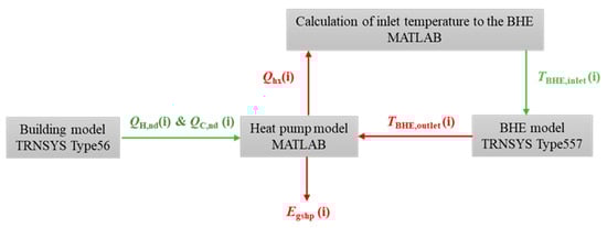
Figure 1.
Flowchart of conducted analysis.
2.1. Building Model
To simulate the realistic operation of a ground-coupled heat pump, the heating and cooling energy requirements for achieving thermal comfort of the observed building had to be determined and used in other models as input data. Data on heating and cooling energy were obtained from another study [25], which conducted hourly energy simulations of the reference nearly zero energy of a single family house in continental Croatia (Figure 2). The floor area of the observed house is 232 m2. The annual heating energy needs are 4477 kWh while cooling energy needs are 17,727 kWh. The heat pump system operates 4018 h/year in the heating regime and 4558 h/year in the cooling regime.
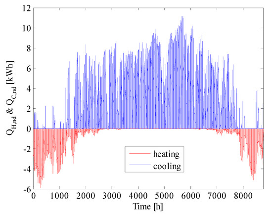
Figure 2.
Hourly heating and cooling needs of the reference nZEB single family house in continental Croatia.
2.2. Heat Pump Model
A ground-coupled heat pump model was developed to simulate heat pump operation and calculate energy consumption based on variable heating and cooling factors (COP and EER) of the pump. COP and EER are each a function of outlet fluid temperature from the borehole and the supply water temperature that needs to be provided to heating and cooling elements (e.g., radiators, fan coils), as shown in Figure 3.
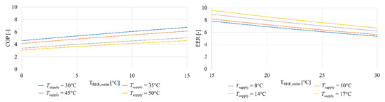
Figure 3.
COP and EER as a function of supply water temperature provided to heating and cooling elements and outlet fluid temperature from the borehole. The plotted values are provided from the manufacturer’s data sheet for the heat pump BlueBox Omega Sky Xi LGW.
The supply water temperature in the heating regime is set to vary based on external air temperature according to the heating regulation curve. Hourly weather data for a typical meteorological year in Zagreb were used. The supply water temperature in the cooling regime was assumed to be constant and set at 8 °C. The borehole outlet fluid temperature was determined from a BHE model, as described later. The energy that needs to be exchanged with the ground ( in heating and in cooling) was calculated according to (1) and (2), based on heating and cooling energy needs as well as hourly COP and EER values.
Repeating the outlined process for an entire simulated year requires calculating the new fluid inlet temperature to the borehole for every subsequent time step. To accomplish that, the TRNSYS model was connected to MATLAB R2015a code using the Type155 component to calculate the inlet temperature of the fluid entering the borehole at every time step. The fluid inlet temperature was calculated based on the outlet temperature of the previous step and the heating and cooling energy exchanged between the heat pump and BHE, according to (3). Energy consumption of the heat pump was calculated according to (4) as a function of building-side energy needs and simulated COP and EER. Additionally, the energy consumption of a circulation pump was also calculated, as it can significantly impact the overall system energy consumption. The energy consumption of the circulation pump was calculated using (5), in which the circulation pump efficiency () was set to 0.8:
2.3. Borehole Model
Simulation of borehole heat exchanger operation was conducted using the TRNSYS 17 software, specifically the Type557a subroutine, which models a vertical heat exchanger that exchanges heat with the surrounding ground. The subroutine uses Hellstrom’s duct heat storage model [26] to simulate the thermal behavior of boreholes. Heat transfer in a borehole is driven by convective heat transfer in fluid and conductive heat transfer to the ground. In the case of more than one borehole, the program assumes that all boreholes are placed uniformly within a cylindrical storage volume of ground. The ground is considered homogeneous across this volume. Also, the thermal capacitance of the borehole is neglected, which can slightly impact the results when transient events occur. In addition to BHE geometry, other inputs for Type557 include thermal properties of the ground, BHE depth, mass flow rate, and inlet temperature in the borehole. The main output from the borehole simulation is the fluid outlet temperature (fluid exiting the borehole). The ground-source heat pump model later uses this output to calculate heat pump efficiency and operational costs for heating and cooling. The simulation time step was set to 5 min to capture the system operation dynamics properly.
Model Validation
The borehole model was validated using the measured data from the borehole installed in Brezice, Slovenia. It consists of a 50 m deep single U-tube. The measured data were acquired from the thermal response test (TRT), during which the inlet and outlet temperature of fluid were measured. The measurement time step was 5 min with a total measurement time of 70 h. The same time step and simulation time were also applied for validation purposes in the TRNSYS simulation. The comparison results (Figure 4) show very good agreement between the simulated and measured data. Quantifying model accuracy required calculating the coefficient of the variation of the root mean square error (CVRMSE) according to (6), which turned out to be 9.20%, demonstrating good accuracy.

Figure 4.
Validation of the TRNSYS borehole heat exchanger model using measured thermal response test data for inlet and outlet temperatures.
2.4. Sensitivity Analysis
Sensitivity analysis identifies parameters that have the greatest influence on the observed output parameter, which allows a better understanding of improving an observed system. Local sensitivity analysis is performed by varying only one parameter while keeping the other parameters constant. Changing the selected input parameter causes a difference only in the output value. Quantifying the influence of a single input parameter requires introducing the influence coefficient (IC). The influence coefficient expresses the output percentage change in cases where the input parameter is adjusted by 1%. It is used to measure the influence of a certain parameter and how the observed parameter is rated compared with other influential parameters. The bigger the influence coefficient for a parameter, the greater its impact on the observed output. The most used expression for the influence coefficient is (7). This form of the influence coefficient is dimensionless, enabling mutual comparison of the influence of different input parameters. Referent values of parameters and the range of parameter values used in local sensitivity analysis are described in Section 2.5.
Global sensitivity analysis considers the simultaneous variation of all influential parameters, capturing their possible interaction. It is, therefore, more advanced and demanding than local sensitivity analysis, and results can easily differ between the local and global sensitivity analysis. The global analysis conducted in this study is known as the Morris method [27]. The method works by sampling a set of initial values of parameters within their defined ranges of possible values and calculating the associated output. In the next steps, the values of the input parameters are changed one by one, where for each change of parameter, the resulting change in output is captured and compared with the previously calculated output. This process continues until all parameters within the observed set of initial values are changed. The procedure is repeated r times, each time with a different set of initial values. That leads to a number of r (k + 1) runs, where k is the number of input parameters. The observed output parameter in this study is heat pump energy consumption. The defined range of possible parameter values is described in Section 2.5, from which the sample for Morris analysis was created. A measure of parameter importance is the mean absolute value of the elementary effect, and this was calculated for each parameter according to (8), while the elementary effect was calculated using (9). Sensitivity analysis of pipe parameters on heat pump energy consumption was investigated under three typical ground thermal conductivities in Croatia: 1.62 W/(m K), 1.819 W/(m K), and 2.7 W/(m K) [28].
2.5. Borehole Heat Exchanger Configurations
The impact of four different borehole heat exchanger parameters on overall system energy consumption was analyzed: pipe diameter, pipe wall thickness, pipe thermal conductivity, and distance between pipes (Figure 5). The mentioned parameters were varied to achieve a BHE with the best thermal properties. Achieved improvements were compared with the base case BHE using heat pump performance as a comparison criterion. Parameters of the base case BHE in this analysis were obtained from the manufacturer’s data, considered to have an outer diameter of 32 mm, pipe wall thickness of 3 mm, distance between pipes of 60 mm, and thermal conductivity of pipe of 0.4 W/(m K) (A. Rozic, personal communication, 28 June 2022) [29]. Thermophysical properties of the BHE, which were the same for all configurations, are listed in Table 1. The range of values of input parameters (Table 2) was defined so that BHE with any combination of input parameter values from the specified range still fits into the standard borehole diameter of 152 mm. The maximum value of the studied pipe thermal conductivity was set as 3 W/(m K), as shown in [19]. This further increase was not required, as the possible BHE depth reduction adopted an asymptotic value. All configurations were assumed to have the same BHE depth for this analysis, the one defined for the base case BHE (more details in Section 2.6). Referent values of parameters used in local sensitivity analysis correspond to the base case BHE parameters, and the range of parameter values used in local sensitivity analysis correspond to those in Table 2. The range of values from Table 2 was also used to create the sample for global (Morris) analysis.
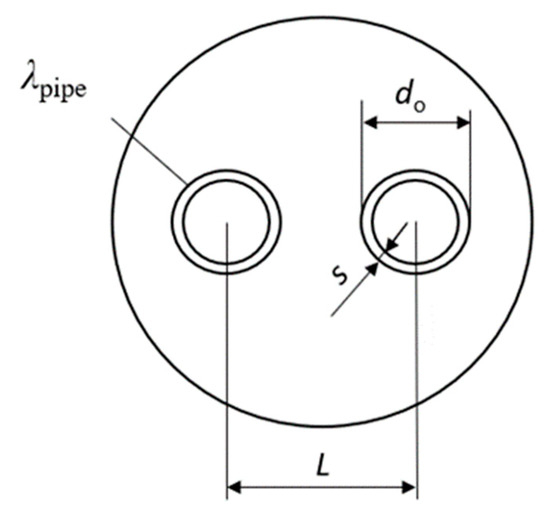
Figure 5.
Cross section of analyzed BHE configurations.

Table 1.
Mutual thermophysical properties of BHE.
Table 2.
Range of values of input parameters for creating various BHE configurations.
As mentioned in the introduction, it is unclear in the literature which flow condition (criterion) is best to set when comparing pipes with different cross sections (for example, when comparing a pipe with increased diameter to the base case). Moreover, different flow conditions were not mutually compared in cases where the impact of diameter was observed. These effects can be important for evaluating BHE effectiveness (in the form of heat exchange with the ground or heat pump energy consumption). To address this issue, the analysis compared three different flow conditions in cases where the influence of pipe diameter was analyzed. Analyzed flow conditions include constant fluid volume flow rate, constant Reynolds number, and constant velocity condition. For this analysis, two BHE configurations were compared: base case and modified (with increased diameter). The outer diameter of the modified pipe was 40 mm, while other parameters were assumed to be the same as for the base case pipe. Both configurations were assumed to have the same BHE depth, defined for the base case BHE (more details in Section 2.6). The fluid filling the probe was water, with a density equal to 998.207 kg/m3 and a dynamic viscosity of 0.001 Pas, both defined by a fluid temperature of 20 °C. The volume flow rate for the base case BHE (outer diameter of 32 mm and inner diameter of 26 mm) was set to 0.6 m3/h per borehole, resulting in a Reynolds number of 8161 and a velocity of 0.31 m/s. This flow rate and resulting velocity were chosen because of the study described in [7], where it is concluded that increasing the velocity over 0.3–0.4 m/s does not improve heat extraction from the ground, independently of the BHE depth. Heat exchanged with ground and total system energy consumption were simulated for each configuration and flow condition and compared in order to capture possible differences and conclusions.
2.6. Sizing of Borehole Heat Exchangers
The performance of a ground-coupled heat pump system depends on the depth of the installed BHE. To properly design a borehole field, the heating and cooling energy needs of the building for which the field is designed must be known. Cooling needs are much higher than heating needs, which can pose a challenge for the proper design of the BHE field. Accordingly, the BHE field is primarily designed to satisfy cooling needs, consisting of two boreholes of a certain depth. Furthermore, the thermal resistance of a borehole heat exchanger is a fundamental parameter for evaluating the borehole thermal performance as well as the design of the borehole field for a specific building and purpose. The thermal resistance of a base case BHE was calculated using the line-source formula for a single U-tube BHE developed by Hellstrom [26]. The calculated thermal resistance of the base case BHE is 0.1168 mK/W. Together with monthly heating and cooling needs and peak loads, this parameter was used to design the borehole field. Design of the borehole field was conducted using the Earth Energy Designer, and the desired borehole depth of the base case BHE for the mentioned conditions was set as 228 m. For practical reasons, the required depth was assumed to be divided into two boreholes, each 114 m deep. The calculated depth for the base case BHE was also used in other BHE configurations in cases where the impact of flow conditions was investigated and where the effect of a change of certain parameters on the overall system energy consumption was investigated.
Part of the study investigating the economic aspects, potential investment, and operational savings requires information about possible reductions in borehole depths for modified BHE configurations. Those depths are defined iteratively by attaining approximately the same heat exchanged with the ground for each BHE. To achieve such conditions, fluid temperature profiles through the borehole should be roughly the same for all boreholes for the same time step (as heat exchanged with the ground depends on those temperatures). Given that both heating and cooling regimes are considered and differ significantly in energy needs (Figure 2), only one of the regimes needed to be chosen as a criterion for achieving approximately the same outlet temperatures. Figure 6 and Figure 7 show examples of the effect of thermal conductivity improvement on the borehole fluid outlet temperature, in both the heating and cooling regimes.
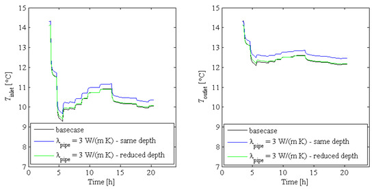
Figure 6.
Comparison of inlet and outlet temperatures between base case BHE and modified BHE with the same and reduced depth heating regime.
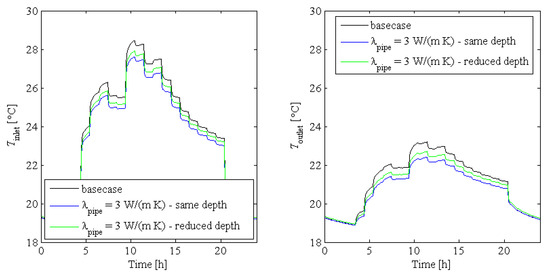
Figure 7.
Comparison of inlet and outlet temperatures between base case BHE and modified BHE with the same and reduced depth cooling regime.
When the thermal conductivity of a BHE pipe is modified, keeping the same depth as in the base case BHE, the fluid outlet temperature is higher in the heating regime and lower in the cooling regime, compared with the base case BHE. This results in higher COP and EER (from Figure 2) and, consequently, lower heat pump energy consumption. In defining reduced borehole depth, the goal was to achieve the same temperatures in one of the conditioning regimes. In this case, the heating regime was chosen, and Figure 6 shows that the BHE with modified thermal conductivity and reduced borehole depth has the same fluid outlet temperature as the base case BHE. What happens with cooling is that even with reduced depth, modified pipes still achieve more beneficial outlet temperatures, allowing lower heat pump energy consumption (Figure 7). If the cooling regime is observed as a criterion for defining borehole depth reduction, even higher depth reduction is achievable, but the efficiency in the heating regime would be compromised (the outlet fluid temperature is lower compared with the base case). Borehole depth reductions for other BHE modifications are defined in the same manner as in this example.
2.7. Financial Input Data
To conduct an economic analysis, costs obtained from manufacturer data (Table 3) were assumed (A. Rozic, personal communication, 1 December 2022). The price of electricity was obtained from the Croatian electricity distributor [30].
Table 3.
Financial input data.
3. Results and Discussion
This section presents a summary and discussion of all the analyzed cases. It highlights the significance of conducting an overall system analysis as opposed to just focusing on the simplified BHE analysis. The discussion also describes the effect of different BHE parameters and flow conditions on the heat pump system performance. Furthermore, the potential savings and trade-offs between investment and operational costs for the analyzed BHE configurations are outlined. Finally, the importance of conducting a global sensitivity analysis instead of a local one is demonstrated.
3.1. The Importance of the Overall System Analysis
As mentioned earlier, most studies investigating the improvement of BHE have focused solely on the BHE component rather than simulating the entire system operation. However, such an approach can lead to unrealistic assumptions about certain parameters. For example, many studies have assumed a constant fluid inlet temperature, which does not reflect actual system operation. Here, we demonstrate the potential drawbacks of such an approach. Figure 8 illustrates inlet and outlet temperatures for one day of the heating regime for two BHE types, the base case (with pipe thermal conductivity equal to 0.4 W/(m K)) and the BHE with modified pipe thermal conductivity (with pipe thermal conductivity equal to 3 W/(m K)). The left plot represents the case where the constant fluid inlet temperature of 6 °C is assumed in both BHE configurations (as typically assumed in other studies) and the resulting outlet temperatures. In contrast, the right plot shows inlet and outlet temperatures in the case of realistic system operation, where the initial inlet temperature was set at 6 °C, and inlet temperatures in other time steps were calculated using (3). When constant inlet temperature was assumed, the increase in pipe thermal conductivity resulted in a 7.57% increase in heat exchanged with the ground (112.85 kWh/day for the base case BHE, compared with 121.39 kWh/day for the modified BHE). However, when a more realistic system simulation was performed, heat exchange was influenced by the heating requirements of the building. In this case, the increase in pipe thermal conductivity results in negligible improvement (0.15%) of heat exchanged with the ground (32.34 kWh/day for base case BHE, compared with 32.39 kWh/day for the modified BHE). The results indicate that the effects of certain BHE improvements can be significantly overestimated if the overall system operation is not simulated. This highlights the importance of analyzing the overall system operation for a realistic evaluation of BHE improvements.
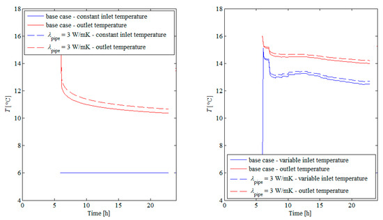
Figure 8.
Comparison of inlet and outlet fluid temperatures for two BHE configurations for presumed constant inlet temperature (left plot) and realistic operation of the system where inlet temperature is calculated from (3) (right plot).
3.2. The Importance and Influence of BHE Parameters on Total System Performance
The study further investigated the impact of various BHE modifications on a whole ground-coupled heat pump system. The realistic performance of the system over a year in both heating and cooling regimes was simulated, where the condition to deliver the same amount of heating/cooling energy was set, irrespective of the BHE configuration. The study went beyond the current literature and evaluated the effectiveness of different BHE configurations more accurately. This part of the study assumed the same volume flow rate (as in the base case) in cases where the BHE pipe cross-section was modified.
The results presented in Figure 9 and Figure 10 show heat exchanged with the ground in heating and cooling regimes, assuming the same depth of 228 m for all configurations. Heat exchange with the ground is shown on the y axis as a function of four influential parameters: thermal conductivity of pipe, pipe diameter, pipe wall thickness, and distance between pipes. The results suggest that changes in certain BHE parameters have a minimal impact on heat exchange with the ground. Once again, the base case was used as the benchmark for comparison in all cases. For instance, when increasing the thermal conductivity of pipe from 0.4 to 3 W/(m K), heat exchange with the ground in the heating regime was improved by 0.12% (rising from 3534.8 kWh/a to 3539.1 kWh/a). The greatest improvement of 0.30% in heat exchanged with the ground was noticed when all parameters were changed simultaneously. Concerning cooling mode, with the increase of pipe thermal conductivity, heat exchange with ground dropped by 0.25% (from 20,555.7 kWh/a to 20,504.7 kWh/a). Reduced borehole thermal resistance led to a smaller temperature difference between the surrounding ground and the fluid flowing inside the borehole heat exchanger. This means that the EER value increased, and smaller amounts of heat were exchanged with the underground for the same cooling output. The greatest improvement of 0.63% in heat exchanged with the ground was also noticed when all parameters were changed simultaneously.
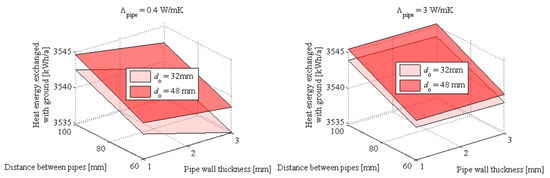
Figure 9.
Heat exchange with the ground as a function of analyzed parameters heating regime. The left plot presents results for the thermal conductivity of the pipe equal to 0.4 W/(m K), and the right for the thermal conductivity of the pipe equal to 3 W/(m K).
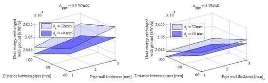
Figure 10.
Heat exchange with the ground as a function of analyzed parameters cooling regime. The left plot presents results for the thermal conductivity of the pipe equal to 0.4 W/(m K), and the right for the thermal conductivity of the pipe equal to 3 W/(m K).
The results presented in Figure 11 show total energy consumption summed for the heating and cooling regimes, assuming the same depth of 228 m for all configurations. Total energy consumption is shown on the y axis as a function of four influential parameters: thermal conductivity of pipe, pipe diameter, pipe wall thickness, and distance between pipes. The results suggest that changes in certain BHE parameters have a minimal impact on total energy consumption. For instance, when increasing the thermal conductivity of pipe from 0.4 to 3 W/(m K), total energy consumption dropped by 1.44% (from 3867.5 kWh/a to 3811.7 kWh/a). The greatest improvement of 5.99% in total energy consumption was noticed when all parameters were changed simultaneously, where 3.65% improvement was due to the heat pump and the rest was due to the circulation pump.
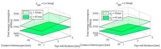
Figure 11.
Total energy consumption as a function of analyzed parameters—summed for heating and cooling regime. The left plot presents results for the thermal conductivity of the pipe equal to 0.4 W/(m K), and the right for the thermal conductivity of the pipe equal to 3 W/(m K).
The results suggest that savings in energy consumption and consequent savings in operational costs are not significant for improved BHE configurations. Hence, potential savings in investment costs related to BHE depth are additionally analyzed here. For this analysis, the BHE depths were reduced in the case of modified BHEs, to attain the same heat exchanged with the ground for all BHE configurations. As a result, the energy consumption and corresponding operational costs of the system were the same for all configurations. The aim was to identify the optimal trade-off between savings in operational (same depth) and investment costs (reduced depth). Estimated costs were calculated considering 10-year system operation. Figure 12 shows the example of 10-year costs (both for heating and cooling) for a BHE with a 32 mm pipe diameter and 0.4 W/(m K) pipe thermal conductivity. Changes in 10-year costs shown in this figure are affected by changes in two parameters: pipe wall thickness and distance between pipes. The results suggest that the most effective strategy for all configurations is to reduce BHE depth to save on the initial investment costs. In particular, if influential parameters from Figure 12 are simultaneously improved, achieved savings in total energy consumption are relatively low (2.83%) if borehole depth is held constant. In contrast, more significant cost savings (9.63%) could be achieved by reducing the borehole depth. Corresponding depth reductions affected by changes in all analyzed parameters are shown in Figure 13.
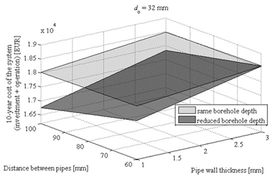
Figure 12.
Estimated 10-year costs for BHE configurations. Results are shown for BHE thermal conductivity of 0.4 W/(m K) and BHE pipe diameter equal to 32 mm.
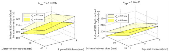
Figure 13.
Iteratively defined depths for BHE configurations—the condition was to achieve approximately the same heat exchange with the ground in the heating regime.
3.3. The Importance of Flow Condition Criteria
The aim of this analysis was to identify the potential differences and benefits of using a certain flow condition when comparing BHE with different pipe cross-sections. Analyzing this factor in the study required comparing the heat transfer rate and energy consumption of a ground-coupled heat pump system using different BHE pipe diameters. Specifically, the base case was 32 mm in diameter, while the modified BHE was 40 mm in diameter. Three flow conditions were analyzed when the pipe diameter was increased: the flow rate, velocity, and Reynolds number. The flow conditions for the base case were predefined and used as a comparison criterion for the modified BHE. The study simulated the system performance over a year in both heating and cooling regimes, with the condition being to deliver the same amount of heating/cooling energy, regardless of the BHE configuration used. The results in Table 4 and Table 5 indicate that heat exchanged with the ground remained nearly constant, regardless of the pipe diameter and flow condition criteria used. The improvements in heat exchange with the ground were below 1% between the base case and all cases with modified diameters. The same conclusion applies to the energy consumption of the heat pump. However, when the energy consumption of the circulation pump is included, some differences can be noticed (Figure 14). The energy consumption of a circulation pump, among other things, depends on the pressure drop that occurs in the BHE. Therefore, it is part of the system where the biggest changes are noticed when pipe diameter and flow conditions are modified. Therefore, considering the total system energy consumption, including the circulation pump, is crucial, especially when changes in the pipe cross-section are investigated. The lowest energy consumption was achieved with the modified BHE that had the same volume flow rate as the base case. On a yearly basis, the modified BHE with a constant flow rate had approximately 2.51% lower energy consumption than the base case BHE (summed for heating and cooling). In contrast, the modified BHE with constant velocity had slightly higher (around 0.49%) energy consumption than the base case BHE. Calculated pressure drops for each configuration are as follows: 63 Pa/m for the base case, 18 Pa/m for qv = const. condition, 45 Pa/m for v = const. condition, and 28 Pa/m for Re = const. condition. The circulation pump operated 4018 h/year in the heating regime and 4558 h/year in the cooling regime.
Table 4.
Numerical values of performance indicators for BHEs with two different diameters and flow conditions—heating regime.
Table 5.
Numerical values of performance indicators for BHEs with two different diameters and flow conditions—cooling regime.
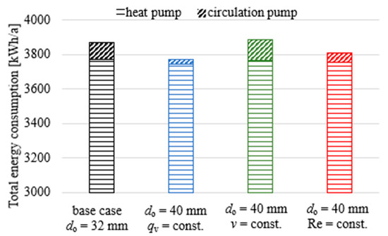
Figure 14.
Differences in total energy consumption for both heating and cooling modes, for base case BHE and BHE with an increased diameter and three different flow conditions.
3.4. The Importance of Global Sensitivity Analysis
This section shows the differences in conclusions regarding the influence of certain parameters depending on the type of sensitivity analysis (local versus global). The order of importance of analysis parameters was investigated for three different thermal properties of the ground to investigate the impact of ground properties on the importance of particular parameters. Analyzed parameters are ranked based on their importance for both sensitivity analyses (Table 6). Conclusions are the same for all ground thermal conductivities, indicating that the ground does not impact the ranking of parameters. However, it can be noticed that the order differs depending on the sensitivity analysis type used. In the case of local sensitivity analysis, the pipe diameter was shown to be the most important parameter, meaning it had the strongest impact on the BHE performance. In contrast, the global sensitivity analysis suggests that the pipe diameter was the second most important parameter, while the distance between pipes had the strongest impact. Such results indicate that input parameters have a strong interaction, which the local sensitivity analysis cannot capture.
Table 6.
Differences between local and global sensitivity analyses regarding the importance of different influential parameters in BHE analyses.
4. Conclusions
The aim of this study was to investigate the performance of ground-coupled heat pump systems subject to four borehole heat exchanger parameters (pipe diameter, pipe wall thickness, distance between pipes, and thermal conductivity) by considering the overall system energy consumption rather than focusing solely on BHE performance. Three different flow conditions (same velocity, same Reynolds, and same flow rate) were also investigated when comparing different pipe cross-sections. The study findings are as follows:
- (1)
- Misleading conclusions are possible if the BHE model and simulations are overtly simplified and decoupled from the rest of the system (heat pump and building). For instance, if a constant inlet temperature was assumed, improvements in pipe thermal conductivity from 0.4 to 3 W/(m K) resulted in a 7.57% increase in the heat exchange rate in BHE, while improvements at a system level were only 0.15%.
- (2)
- The modifications to the analyzed BHE parameters (pipe diameter, wall thickness, thermal conductivity, and distance between pipes) showed a limited impact on overall system performance. The greatest improvement was achieved when all parameters were modified simultaneously, resulting in a 6% reduction in total system energy consumption. These findings indicate that optimizing BHE parameters alone may not necessarily lead to significant improvements in the overall system performance.
- (3)
- The results suggest that flow condition criteria had little impact on heat exchange with the ground or the energy consumption of the heat pump. However, changes in the pipe cross-section and flow condition directly impacted the energy consumption of the circulation pump. When the same flow velocity criteria were used to compare the base case BHE and modified BHE, the total energy consumption of the system was higher for the modified BHE despite better heat exchange with the ground.
- (4)
- An analysis of optimization strategies suggests that potential savings in investment costs outweigh potential savings in operational costs. In particular, savings in total energy consumption are 2.83% for modified BHE compared to the base case if the borehole depth remains constant for the two cases. In contrast, if the borehole depth is reduced for the modified BHE case (maintaining the same heat rate exchanged with the ground as in the base case scenario), cost savings of 9.63% are achieved.
- (5)
- The order of importance of the observed parameters might not be the same, depending on the type of sensitivity analysis used (local versus global). For example, in the case of local sensitivity analysis, the pipe diameter was shown to be the most important parameter, whereas global sensitivity analysis suggests that the distance between pipes had the greatest impact. These results suggest that a notable interaction between influential parameters and the use of local sensitivity analysis may lead to misleading conclusions.
This study offers valuable insights for improving the simulation and evaluation of ground-coupled heat pump performance. The findings can assist in the decision-making process when considering these modifications and related economic benefits.
Author Contributions
Conceptualization, L.M. and T.Z.; Formal analysis, L.M.; Funding acquisition, T.Z.; Investigation, L.M.; Methodology, L.M. and T.Z.; Project administration, T.Z.; Resources, T.Z. and L.B.; Software, L.M.; Supervision, T.Z. and L.B.; Validation, L.M.; Visualization, L.M.; Writing—original draft, L.M.; Writing—review & editing, T.Z. and L.B. All authors have read and agreed to the published version of the manuscript.
Funding
The paper was written as part of the project Development of Innovative Systems for the Use of Geothermal Energy Sources and Energy from Biological Waste−RazInoGeoBio (Project code: KK.01.2.1.02.0314) financed by the Operational Program “Competitiveness and Cohesion 2014–2020” from the European Fund for Regional Development as part of the call KK.01.2.1.02—Increasing the development of new products and services resulting from research and development activities (IRI)—phase II. The authors would like to thank the European Union for funding this project.
Data Availability Statement
The data presented in this study are available on request from the corresponding author.
Conflicts of Interest
The authors declare no conflict of interest.
Nomenclature
| heat energy exchanged with the ground in heating mode [kWh] | |
| heat energy exchanged with the ground in cooling mode [kWh] | |
| heating needs [kWh] | |
| cooling needs [kWh] | |
| heating factor [-] | |
| cooling factor [-] | |
| fluid inlet temperature to the borehole [°C] | |
| fluid outlet temperature to the borehole [°C] | |
| supply temperature to the heating and cooling elements [°C] | |
| fluid mass flow rate [kg/h] | |
| fluid volume flow rate [m3/h] | |
| specific heat capacity [kJ/(kg K)] | |
| ground-source heat pump energy consumption [kWh] | |
| circulation pump energy consumption [kWh] | |
| pressure drop [Pa] | |
| circulation pump efficiency [-] | |
| system operation time [h] | |
| coefficient of the variation of the root mean square error [%] | |
| total number of time steps [-] | |
| measured fluid outlet temperature at i-th time step [°C] | |
| simulated fluid outlet temperature at i-th time step [°C] | |
| mean value of the measured outlet temperature in the observed interval [°C] | |
| impact coefficient [-] | |
| change in output variables | |
| referent value of output variable | |
| change in input variables | |
| referent value of input variable | |
| mean absolute value of elementary effect [-] | |
| number of input variables [-] | |
| elementary effect [-] |
References
- Lucia, U.; Simonetti, M.; Chiesa, G.; Grisolia, G. Ground-source pump system for heating and cooling: Review and thermodynamic approach. Renew. Sustain. Energy Rev. 2017, 70, 867–874. [Google Scholar] [CrossRef]
- Lund, J.W.; Boyd, T.L. Direct utilization of geothermal energy 2015 worldwide review. Geothermics 2016, 60, 66–93. [Google Scholar] [CrossRef]
- Boban, L.; Miše, D.; Herceg, S.; Soldo, V. Application and design aspects of ground heat exchangers. Energies 2021, 14, 2134. [Google Scholar] [CrossRef]
- Yang, H.; Cui, P.; Fang, Z. Vertical-borehole ground-coupled heat pumps: A review of models and systems. Appl. Energy 2010, 87, 16–27. [Google Scholar] [CrossRef]
- Habibi, M.; Hakkaki-Fard, A. Evaluation and improvement of the thermal performance of different types of horizontal ground heat exchangers based on techno-economic analysis. Energy Convers. Manag. 2018, 171, 1177–1192. [Google Scholar] [CrossRef]
- Soltani, M.; Kashkooli, F.M.; Dehghani-Sanij, A.R.; Kazemi, A.R.; Bordbar, N.; Farshchi, M.J.; Elmi, M.; Gharali, K.; Dusseault, M.B. A comprehensive study of geothermal heating and cooling systems. Sustain. Cities Soc. 2019, 44, 793–818. [Google Scholar] [CrossRef]
- Han, C.; Yu, X. Sensitivity analysis of a vertical geothermal heat pump system. Appl. Energy 2016, 170, 148–160. [Google Scholar] [CrossRef]
- Casasso, A.; Sethi, R. Efficiency of closed loop geothermal heat pumps: A sensitivity analysis. Renew. Energy 2014, 62, 737–746. [Google Scholar] [CrossRef]
- Nam, Y.; Chae, H.B. Numerical simulation for the optimum design of ground source heat pump system using building foundation as horizontal heat exchanger. Energy 2014, 73, 933–942. [Google Scholar] [CrossRef]
- Noorollahi, Y.; Saeidi, R.; Mohammadi, M.; Amiri, A.; Hosseinzadeh, M. The effects of ground heat exchanger parameters changes on geothermal heat pump performance—A review. Appl. Therm. Eng. 2018, 129, 1645–1658. [Google Scholar] [CrossRef]
- Hein, P.; Kolditz, O.; Görke, U.J.; Bucher, A.; Shao, H. A numerical study on the sustainability and efficiency of borehole heat exchanger coupled ground source heat pump systems. Appl. Therm. Eng. 2016, 100, 421–433. [Google Scholar] [CrossRef]
- Boban, L.; Soldo, V.; Fujii, H. Investigation of heat pump performance in heterogeneous ground. Energy Convers. Manag. 2020, 211, 112736. [Google Scholar] [CrossRef]
- Kurevija, T.; Macenić, M.; Borović, S. Impact of grout thermal conductivity on the long-term efficiency of the ground-source heat pump system. Sustain. Cities Soc. 2017, 31, 1–11. [Google Scholar] [CrossRef]
- Zhang, W.; Yang, H.; Lu, L.; Fang, Z. Investigation on influential factors of engineering design of geothermal heat exchangers. Appl. Therm. Eng. 2015, 84, 310–319. [Google Scholar] [CrossRef]
- Makasis, N.; Narsilio, G.A.; Bidarmaghz, A.; Johnston, I.W. Ground-source heat pump systems: The effect of variable pipe separation in ground heat exchangers. Comput. Geotech. 2018, 100, 97–109. [Google Scholar] [CrossRef]
- Javadi, H.; Ajarostaghi, S.S.M.; Rosen, M.A.; Pourfallah, M. Performance of ground heat exchangers: A comprehensive review of recent advances. Energy 2019, 178, 207–233. [Google Scholar] [CrossRef]
- Bassiouny, R.; Ali, M.R.O.; Hassan, M.K. An idea to enhance the thermal performance of HDPE pipes used for ground-source applications. Appl. Therm. Eng. 2016, 109, 15–21. [Google Scholar] [CrossRef]
- Yoon, S.; Lee, S.R.; Kim, M.J.; Kim, W.J.; Kim, G.Y.; Kim, K. Evaluation of stainless steel pipe performance as a ground heat exchanger in ground-source heat-pump system. Energy 2016, 113, 328–337. [Google Scholar] [CrossRef]
- Narei, H.; Fatehifar, M.; Ghasempour, R.; Noorollahi, Y. In pursuit of a replacement for conventional high-density polyethylene tubes in ground source heat pumps from their composites—A comparative study. Geothermics 2020, 87, 101819. [Google Scholar] [CrossRef]
- Jahanbin, A. Thermal performance of the vertical ground heat exchanger with a novel elliptical single U-tube. Geothermics 2020, 86, 101804. [Google Scholar] [CrossRef]
- Eswiasi, A. Novel Pipe Configuration for Enhanced Efficiency of Vertical Ground Heat Exchanger (VGHE). Ph.D. Thesis, University of Victoria, Victoria, BC, Canada, 2021. [Google Scholar]
- Bouhacina, B.; Saim, R.; Oztop, H.F. Numerical investigation of a novel tube design for the geothermal borehole heat exchanger. Appl. Therm. Eng. 2015, 79, 153–162. [Google Scholar] [CrossRef]
- Zhou, H.; Lv, J.; Li, T. Applicability of the pipe structure and flow velocity of vertical ground heat exchanger for ground source heat pump. Energy Build. 2016, 117, 109–119. [Google Scholar] [CrossRef]
- Kim, M.J.; Lee, S.R.; Yoon, S.; Go, G.H. Thermal performance evaluation and parametric study of a horizontal ground heat exchanger. Geothermics 2016, 60, 134–143. [Google Scholar] [CrossRef]
- Zakula, T.; Bagaric, M.; Ferdelji, N.; Milovanovic, B.; Mudrinic, S.; Ritosa, K. Comparison of dynamic simulations and the ISO 52016 standard for the assessment of building energy performance. Appl. Energy 2019, 254, 113553. [Google Scholar] [CrossRef]
- Hellström, G. Ground Heat Storage: Thermal Analyses of Duct Storage Systems. Ph.D. Thesis, Lund University, Lund, Sweden, 1991; p. 310. Available online: https://lucris.lub.lu.se/ws/portalfiles/portal/6178678/8161230.pdf (accessed on 2 September 2021).
- Campolongo, F.; Cariboni, J.; Saltelli, A.; Schoutens, W. Enhancing the Morris Method. Sensit. Anal. Model Output 2005, 369–379. [Google Scholar]
- Soldo, V.; Boban, L.; Borović, S. Vertical distribution of shallow ground thermal properties in different geological settings in Croatia. Renew. Energy 2016, 99, 1202–1212. [Google Scholar] [CrossRef]
- Rozic, A.; Telur Ltd., Zagreb, Croatia. Personal communication, 2022.
- HEP ELEKTRA d.o.o.—Tarifne Stavke (Cijene). Available online: https://www.hep.hr/elektra/kucanstvo/tarifne-stavke-cijene/1547 (accessed on 19 January 2023).
Disclaimer/Publisher’s Note: The statements, opinions and data contained in all publications are solely those of the individual author(s) and contributor(s) and not of MDPI and/or the editor(s). MDPI and/or the editor(s) disclaim responsibility for any injury to people or property resulting from any ideas, methods, instructions or products referred to in the content. |
© 2023 by the authors. Licensee MDPI, Basel, Switzerland. This article is an open access article distributed under the terms and conditions of the Creative Commons Attribution (CC BY) license (https://creativecommons.org/licenses/by/4.0/).