Fatigue Strength Analysis of a Prototype Francis Turbine in a Multilevel Lifetime Assessment Procedure Part III: Instrumentation and Prototype Site Measurement

Abstract

Part I of this series of publications addressed the background and fundamentals of the lifetime assessment of prototype Francis turbines. Part II concentrated on the developed methods of numerical calculation and assessment procedures. The present contribution (Part III) deals with the instrumentation and the metrological range of the assessment procedure. The most important sensors, measurement tools, and data acquisition units are presented (background). The instrumentation of the prototype Francis turbine is used, on the one hand, for machine unit monitoring and plant operating and, on the other hand, for generating measurement data to validate and adjust/correct the numerical simulations. Measurement data form the basis for further evaluations at various levels. A wide variety of measured variables are required to carry out the remaining lifetime of a component using fatigue analysis. Those variables include pressure and acceleration signals, vibration monitoring, and strain gauge applications for mechanical stress analysis. The available measurement signals are divided into groups based on the developed method. Thus, already-available data from the control room are compared with machine monitoring and temporarily measured data. The correlation of all available data is essential today to determine an exact idea of the occurring flow phenomena and their effects on the mechanical stresses on the component. This interaction of the different data sources and, subsequently, the use of selected quantities for the numerical calculation are part of the newly developed concept for fatigue strength analysis of mechanical components of a turbine unit (methods). The results of this journal article are divided into the discussion of the necessary instrumentation and mounting of the sensors and into the evaluation, presentation, and interpretation of the measurement data. In addition, a fatigue strength assessment is made at the position of the strain gauges. These results serve as a basis for validating the numerical stress calculation. It is worth mentioning that the validation of the numerical results and the discussion of the deviations and error consideration is carried out in Part IV of this publication series (results). This journal article of the series on condition assessment of prototype Francis turbines ends with a discussion of the results and conclusions for further data processing (conclusion).

1. Introduction

The present paper is part of a series of several publications on the subject of fatigue strength analysis of prototype Francis turbines in a multilevel lifetime assessment procedure. PART I [1] contains the chosen approach’s developed method and primary considerations, while PART II [2] is dedicated to the numerical approach. PART III presents the required sensor installation in the hydropower plant and the analysis based on measured data. References between the individual parts are repeatedly used to remain focused on the essential core of the respective paper. The explanations and results in this paper refer to hydropower plant 2, described in detail in SECTION 2.2. of PART II [2].

This introduction aims to provide a concise historical overview of metrological investigations conducted in detecting flow phenomena relevant to damage in hydraulic machines, explicitly focusing on the lifetime analysis of Francis impellers.

With the advent of the liberalization of the European electricity market and the rise of new renewable energy sources (such as wind and photovoltaic), hydropower faces the challenge of operating its machines in off-design operating points. Francis and pump turbines are particularly susceptible to this mode of operation, as their runner blades cannot be adjusted to accommodate the altered flow regime. Consequently, early investigations were carried out to understand the flow phenomena occurring in these unconventional operating points. Detailed studies have been and continue to be conducted on flow separation, residual swirl leading to vortices and cavitation phenomena. As early as 2007, Ref. [3] demonstrated how blade trailing edge separation and the classical Von Karman vortex shedding frequency associated with it could lead to resonance problems and crack formation. Ref. [4] also reported on crack initiation in a Francis runner after in situ repair. At that time, the phenomenon of the draft tube vortex was known, but not its effects on crack initiation and, thus, on the component’s lifetime. Metallurgical investigations were, therefore, carried out in addition to calculations. Blade failure was attributed to part-load operation and unfavorable flow conditions. A key issue in determining blade cracks in the fatigue strength simulation are the frequencies and amplitudes of the dynamic loads that occur, as shown by [5]. The first approaches to consider those effects already at the design phase were reported by [6] in 2012. Recent investigations on the laboratory test rig model [7] show that for this flow phenomenon, not only does the already known rotational frequency of approximately $(0.2-0.4)·n$ occur, where n represents the rotational speed of the Francis turbine, but also higher proportions resulting from the self-rotation and the shape of the vortex. These considerations of unique flow phenomena allow the identification of individual frequencies from an overall frequency spectrum of the machine.

The first metrological and numerical investigations of the various operating points also began during this period [8]. In the beginning, these studies focused on the challenges at the transient operating points, such as speed-no-load or start and stop of the machine, since this was assumed to have the most damaging influence on the remaining lifetime of a Francis turbine [9]. In order to study these influences better, laboratory tests on model turbines were conducted. In particular, the shutdown of a turbine with a short-term increase in speed and the associated dynamic stresses on the runner represents a wide range of investigation possibilities. Ref. [10] is dedicated to the associated pressure fluctuations and mechanical stresses in this context and presented initial results in 2014. In parallel, the investigations of dynamic stresses continued and focused on a wide variety of load points [11,12]. According to current theories, this is important, since dynamic stresses are responsible for determining the remaining lifetime. However, the first studies were conducted on laboratory test rigs, which again have a scaling problem. A general study on this is presented in [13].

The quintessence of these investigations results in predicting the lifetime of Francis turbines under the previously mentioned conditions. For more than ten years, the influence of various parameters on the residual lifetime has been investigated. Suppose a deviation is made from the classical design of water turbines according to the medium stress concept in the direction of fatigue strength. In that case, entirely new challenges arise in determining dynamic stresses. As already shown in Part I of this paper series, different flow phenomena occur in the individual load steps and cause those pressure fluctuations, which in turn lead to dynamic mechanical stresses responsible for the lifetime reduction. This is shown in the study [14] from 2012 and subsequently from 2014, presented in [15]. Mechanical stresses depend on the size of the structure, since the mass, damping, and stiffness matrix cannot be easily scaled. Many examinations have been conducted on prototype machines [16,17]. There is still a distinction between whether strain gauge measurements exist directly on the runner [18] or not.

The subject of several review papers is the influence of singularly damaging flow phenomena and their combinations on the operation of a Francis turbine at different operating points. For example, the transient effects, such as start–stop or load rejection of a machine, are addressed in [19]. How these effects can be transferred from the fluid domain to the component structure and which procedures or methods have been applied to date are described in [20]. These mathematical procedures and methods require solid validation, which can only occur in prototype hydropower plants to avoid scaling effects between the model and prototype runner. Experimental tests and measurement procedures in real plants are described in [21]. The literature shows that the distinguished influence of the draft tube vortex on the lifetime of Francis turbines has recently become a topic of interest. This flow phenomenon plays a significant role, especially in Francis turbines with a higher specific speed $n_q$. The possibilities of detection in hydraulic machines are described in a review paper [22]. The publications cited give a comprehensive overview of the methods and procedures used in the field of flow patterns and possible effects on the element structure.

In recent years, the need for stress–strain measurements on the runner under actual operating conditions has been acknowledged in order to validate the calculation methods and to determine the associated vibration modes and natural frequencies in the frequency domain. The possibilities of such measurements are, of course, limited and not feasible for every runner. A suitable hub design is needed to accommodate the data logger and power supply and to protect them from the flow. In addition, the boundary conditions for the strain gauges are extremely harsh, so they can only be in use for a short time period. Examples of such plant measurements with strain gauges and their evaluations are presented in refs. [23,24]. In this context, of course, the issues of “oscillating water masses”, stiffness effects of the labyrinth seals, and system damping due to the lubricant film thickness in the bearings must also be taken into account. While these factors are automatically included in the prototype measurements, they represent an enormous challenge in the development of computational models.

This short literature review shows that there is still room for further method development and research work about the lifetime assessment of Francis turbines. Especially in the area of turbine measurement technology, data acquisition and storage, on-site processing, and integration into the operating SCADA system, many questions are still unanswered. The sampling rate and automated detection of damage mechanisms will still need to be investigated for longer. It can already be seen that only a combined approach of calculation and measurement will lead to the goal. Accordingly, further plant measurements on selected machine units are of utmost importance.

This paper series is dedicated to this comprehensive question, but it is so voluminous that it has to be divided into several parts. This articles content includes the plants metrological equipment for the validation measurement, the measurement procedure, and the presentation and evaluation of the results. The structure is as follows.

Section 1 provides a literature review of the latest publications on the experimental validation of a Francis turbine lifetime assessment. An emphasis on the proposed evaluation method going beyond the State-of-the-Art shows the heuristic approach focusing on the metrological part (see Figure 1).

Section 2 describes the metrological process in the selected hydropower plant, consisting of the measurement site identification, sensor selection and application, and measurement procedure to obtain the necessary data to validate the calculations. In addition, sensors are placed in those areas and cross-sectional planes, which will be needed as boundary conditions for the numerical simulation later.

In Section 3, the measurement results at several operating points and different aspects are presented. Correlations of distinct sensor data illustrate a singular flow phenomenon from different points of view and under the influence of air injection. Furthermore, the lifetime at strain gauge spots is evaluated. Extrapolation in the direction of the hotspot is omitted because the concept of stress-intensity factors is too imprecise. The conventional approach is considered critical in this case and will be explained in more detail in Section 3.3.2.

Section 4 discusses the topic of sensor selection and a possible extension of the diagnostic system. Based on the predefined sensor groups and the subsequential data time series as well as frequency spectra, a correlation matrix can optimize the selection of measurement signals for a diagnostic system. A substantive discussion on the stress-intensity factor rounds out the chapter.

Section 5 deals with the conclusions of the findings and gives recommendations for further procedure.

In Appendix A, the sensor installations at the hydropower plant are shown. Additionally, application notes and sensor characteristics are presented. In order not to distract the paper content too much, it was decided to add this information at the end within the Appendix A.

Beyond the State-of-the-Art Investigations—The Transient Assessment Model

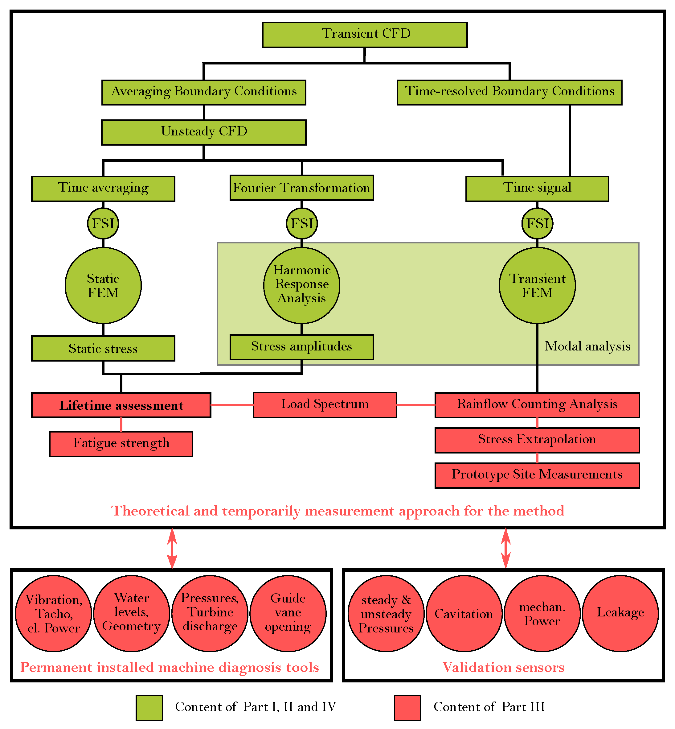
Figure 1 shows the content of this paper quite clearly. The upper green area represents the simulation level, while the red area in the figure’s lower half represents the process’s metro logical part. It is clear from this figure that both numerical simulation and metrological validation are necessary for determining the service life of the component (Francis turbine). This necessity and interplay between simulation and measurements will be described and discussed in more detail later on.

Figure 1. Measurement path of assessment method.

Figure 1. Measurement path of assessment method.

As already presented in PART I [1] and PART II [2], the transient mechanical stress calculation is a new approach to the determination of the lifetime of a Francis turbine. Especially the time-resolved boundary conditions need reliable metrological validation. Therefore, boundary conditions, monitoring points and simulation results must be validated with measurement data in the best possible way. Since measurement and simulation always diverge, performing an accurate error analysis with subsequent uncertainty evaluation is essential.

Diverse data sources can be used, e.g., operational data processed in a SCADA system or additionally installed monitoring sensors providing mechanical protection for the machine. In some cases, however, additional sensors are needed to provide the necessary time series data for the validation. These additionally required sensors can be subdivided again into those that can only be used temporarily. Moreover, those sensors can be mounted permanently on the outside of the machine set. This group of sensors also has the potential to be included in the list of operational data if it proves helpful.

The selection of the required sensors and measuring devices, as well as the further processing of the obtained data, is described in this article. Due to the large number of different flow phenomena which can influence the operation of the machine and are responsible for the decrease in service life, adapted measurement variables and sampling rates are used. In the context of the method development for determining the residual lifetime of a component, it primarily concerns the collection of the necessary signals and their temporal resolution. In many cases, the existing operating data is too coarse in its granularity to be used meaningfully in method development. Therefore, some operating signals are recorded additionally in higher resolution to ensure proper processing. In the first step, a load increase method is applied to investigate the behavior at different operating points in more detail. Subsequently, monitoring systems for continuous operation could be developed from this.

2. Measurement Process

The focus of the underlying research project is to establish the correlation between machine operation and lifetime for all operational points. As shown previously and as documented by the cited publications, the behavior of the machine unit relates to different flow patterns and resulting loads. The question arising at this stage is the proper instrumentation to cover all different instabilities and loads to get an overall impression of the condition of the machine or its components. One has to take into account that various flow phenomena would require different measurement techniques to examine their influence. Moreover, the question whether important investigation parameters can be measured directly or indirectly has to be answered. Another important point is the occurrence of more than one different flow phenomenon at one operation point, as shown in TABLE 2 in PART I [1], thus making the prototype measurement and data interpretation much more difficult during post-processing.

Based on the already-performed prototype measurements, the selected sensor installation and measurement procedure is discussed to show the complex task of attempting to collect the correct data at the proper position. A well-prepared instrumentation and workflow plan is essential for the acquisition of useful data.

2.1. Instrumentation Overview and Sensor Application

As mentioned in the introduction, all figures, interpretations, and results refer to hydropower plant 2, which has already been described in detail in SECTION 2.2 of PART II [2] of this paper series. This plant can be used as a representative for all other hydropower plants, as the installation of the measurement equipment can only be limited by the accessibility of the machine unit. However, all stress analyses and evaluations remain unaffected, and thus, retain their validity.

Figure 2 shows the different positions with their measurement signals at the machine unit and turbine cross section.

To organize the multitude of signals, a suitable classification system based on the considerations above was developed.

• Permanent installed sensors to acquire operational data.
  Usually, those sensors measure operating variables, such as water levels, flow rates, drop heights, angle of the guide vanes, or electrical power. Mostly, they lack appropriate data granularity for the methodology as the sampling rate is rather low. However, they are still usable as CFD boundary conditions or to validate the global CFD-simulated parameters. The list of used sensors and their quantity is visible in the first block of Table 1. The data storage source is usually the server storage media within the SCADA system.
• Permanent machine diagnosis sensors.
  Permanent machine diagnosis consists of a set of various sensors which are attached to different components to measure the behavior directly or indirectly. The time series of the sensor signals are processed (for example, transfer into frequency domain) to gain more insight into the component condition to avoid unexpected breakdowns. These signals are also the base for any further developed maintenance strategy. The following positions on hydraulic machines or their operating parameters are already frequently considered for permanent machine diagnostics:

  –

  Detecting the position and vibration of the Runner [25,26].

  The method detects some sources of error in the shaft line, such as off-design regions, imbalances caused by mass displacement or shaft misalignment, shear pin malfunctions, or vibrations at the guide vane apparatus and radial bearing problems.

  –

  Detecting vibrations and dynamic pressures at the head cover and/or the draft tube cone [25,26].

  Erosion and abrasion phenomena, such as cavitation, sand particles, etc., damage the water-carrying components of a hydraulic machine and, thus, of course, the runner itself. They lead to material loss at particularly exposed locations or sealing gaps, and thus, reduce the efficiency of the machine unit. Progressive erosion even forces a shutdown and repair of the unit. Altered gap dimensions or clearances can lead to vibrations in housing parts. Acceleration sensors monitor vibrations at the head cover and the draft tube cone. Changes in the frequency or amplitude of those signals are used for monitoring and operating the machine unit.

  –

  Checking the seal ring gap.

  Labyrinth seals are used in Francis turbines to limit gap water flow and increase turbine efficiency. Sensors that monitor the sealing gap assist in machine monitoring in terms of efficiency.

  –

  Measuring Temperatures at Thrust and Guide Bearings.

  Failure sources, such as insufficient lubricant film thickness, mechanical overload, or bearing material fatigue, lead to difficulties in keeping the bearing oil film stable, and therefore, cause a temperature increase in hydraulic oil and the bearing itself.

  –

  Detecting the oil film thickness at thrust bearings.

  A collapsing oil film thickness damages the thrust pads in axial bearings, and thus, inevitably stops the machine unit. If this is not detected and corrected in time, bearing or even damage to the rotor is unavoidable. Appropriate installed vibration displacement sensors prevent this by measuring the axial bearing distance or the oil film thickness.

  –

  Detecting vibrations in the stator frame of a generator [25,26].

  The generator of a hydraulic machine set is subject to many magnetic and thermal cycles during its lifetime, which can lead to the loosening of parts and vibrations. These occurring vibrations as indicators of approaching damage to the generator stator can be detected using accelerometers and implemented in the unit’s machine diagnostics.

  –

  Detecting vibrations in stator bars and end windings [25,26].

  Stator bars and subsequential end windings are subject to electromagnetic, mechanical, and gravitational forces during the regular operation of a hydroelectric generator, which can cause the stator bar splice to become detached. The consequences are vibrations and insulation losses, which in turn cause the unit to shut down and result in a longer repair time.

  –

  Checking the air gap between the generator rotor and stator.

  The air gap between the generator rotor and stator is an essential measure of the efficiency of a hydroelectric generator. The smaller the air gap is, the lower the losses in this component. Therefore, measuring the air gap is an important indicator for the quality assessment of a hydropower generator. Depending on the design, between one and sixteen sensors are used around the circumference of the generator stator. They measure instantaneous values, subsequently treated as statistical values, such as min, max, and average values. Furthermore, the roundness of the rotor, as well as the stator, can be verified.

  –

  Monitoring partial discharge behavior at the generator.

  Partial discharge measurements are used to determine the quality of the insulation of a hydropower generator. These are based on the corona effect and represent local electrical discharges. They can occur in cavities within the insulation system or at microcracks in the insulation itself. The number of detected partial discharges between the rotor and stator measures the insulation quality and can, therefore, be integrated into a modern maintenance management system. However, no standard for comparative values exists, so company or operator know-how is needed.

  –

  Monitoring operational parameters.

  In the SCADA system of modern hydropower plants, necessary operating variables are recorded and stored. These are parameters such as level heights of reservoirs or river stretches, rotational speed, power output, various generator voltages, bearing temperature, pressures, and positions at the valves. These measured variables are sampled at a higher sampling rate, but are then usually only stored at 1 Hz or less in the long-term storage systems of the power plant operators.

  Today, these measurement techniques and related sensors are correlated in terms of condition monitoring. Additional information on the powerhouse control system and market information leads to developing enhanced maintenance strategies such as predictive maintenance. In the present research study, the used permanent monitoring sensors are listed in block 2 of Table 1. The data storage source is mostly a separate server structure media and some processed data are sometimes exported to the SCADA system. However, usually, these signals are separately processed as their main purpose is the machine protection against mechanical disrupture.
• Temporary measurements for component assessment.
  Temporarily direct attached sensors for component assessment determine the mechanical stresses utilizing strain gauges or runner properties, such as the natural frequency by using accelerometers. So-called direct measurement methods are used here. This form of measurement data determination should be considered first, as far as possible, because they provide the most original values. However, the application of such sensors is limited in hydraulic machines, as the parts in contact with water do not provide an ideal environment for using this direct measurement method. The dwell time of such sensors is limited to a few hours and can only be provided for initial measurements. The data storage is usually a data logger, as telemetry systems are most likely to be used in the presence of a hollow shaft. Very rarely, the signal from the telemetry system is transmitted via the waterway, as this is very complex and costly. Moreover, it only makes sense to use it with larger turbine units. In the present research project, strain gauges and acceleration sensors were installed on the impeller and data sampling was carried out using a data logger. The storage medium was a conventional SD card.
• Temporary validation sensors.
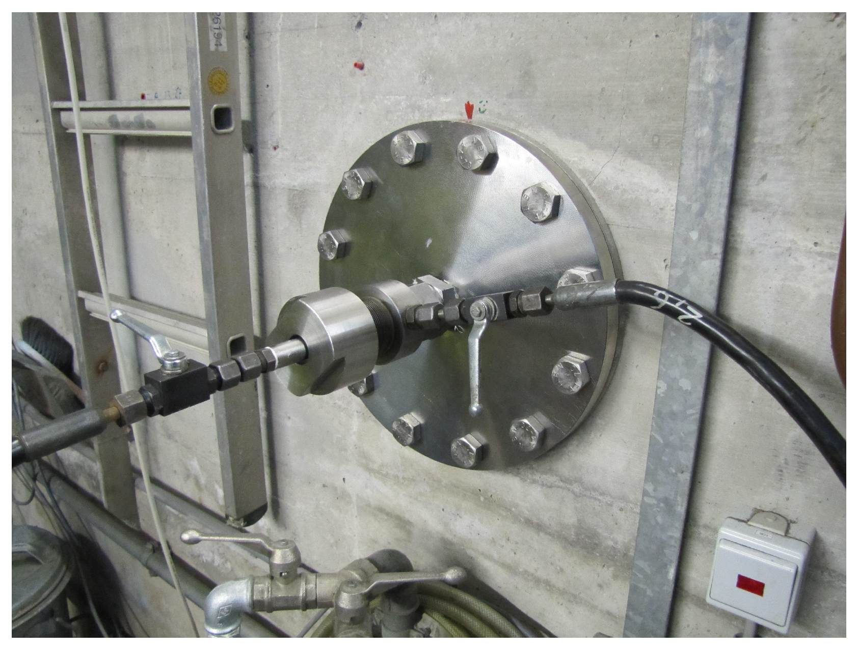
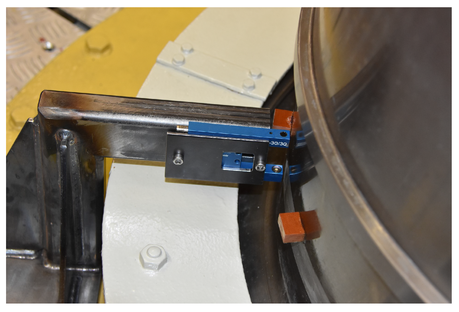
  This group uses sensors that can be externally attached to the machine unit. They serve as boundary conditions for the CFD simulations and validation values for the integral calculation parameters or as a direct comparison with monitoring points. The number and mounting options on the machine depend very much on accessibility. In addition, these sensors can be included in the list of operating data if this proves helpful. A unique feature of this research project was the non-contact measurement of the mechanical torque on the shaft. This was possible because there was a sufficiently long, exposed turbine shaft between the lower generator and turbine bearing. The background to this measurement is splitting the outputs ($P_{hydraulic}$, $P_{mechanic}$, $P_{electric}$), and thus, the possibility of separate efficiency consideration. This means the hydraulic efficiency can be determined separately for the first time. Furthermore, it is interesting to see to what extent existing flow phenomena are responsible for power fluctuations at the generator. Group 4 of Table 1 shows the number of sensors.

In total, a list of 29 parameters (see Table 1) comprising a quantity ($Qty$) of 53 sensor signals with different sampling rates should give the possibility to evaluate the behavior of the runner and guide vanes of the unit.

Table 1. List of measurement signals and usage.

No.	Signal	Qty	Position	Signal Type	Usage
Permanent Operational data
1	$z_{HW}$	1	head-water level	geodetic height in $\mathrm{m}$	operating point
2	$z_{TW}$	1	tail-water level	geodetic height in $\mathrm{m}$	operating point
3	$a_0$	1	wicket gate	choke length in %	operating point
4	Q	1	in the spiral case	discharge in ${\mathrm{m}}^3/\mathrm{s}$	operating point
3	$p_{TCV}$	1	before turbine closing valve	pressure in $\mathrm{bar}$	operating point
4	$p_{SC}$	1	at the spiral case	pressure in $\mathrm{bar}$	operating point
7	$p_{RN}$	1	runner entry	pressure in $\mathrm{bar}$	pressure distribution in side chamber
8	$p_{CO}$	1	turbine cover	pressure in $\mathrm{bar}$	pressure distribution in side chamber
9	$p_{con.2}$	1	draft tube cone	pressure pos. 2 in $\mathrm{bar}$	DTV, FSO, SPP
10	n	1	turbine shaft	speed in ${\min }^{-1}$	operating point, mechanical power
11	$P_{el}$	1	generator	electrical power in $\mathrm{MW}$	electrical power, efficiency
Permanent machine diagnosis sensors
12	$r_{TH{B}_{x,y}}$	2	turbine bearing	displacement in x,y in $\mathsf{\mu }\mathrm{m}$	relative shaft vibration
13	$a_{TH{B}_{x,y}}$	2	turbine bearing	velocity in x,y in $\mathrm{mm}/\mathrm{s}$	absolute bearing vibration
14	$r_{LG{B}_{x,y}}$	2	lower gen. bearing	displacement in x,y in $\mathsf{\mu }\mathrm{m}$	relative shaft vibration
15	$a_{LG{B}_{x,y}}$	2	lower gen. bearing	velocity in x,y in $\mathrm{mm}/\mathrm{s}$	absolute bearing vibration
16	$r_{UG{B}_{x,y,z}}$	3	upper gen. bearing	displacement in x,y,z in $\mathsf{\mu }\mathrm{m}$	relative shaft vibration
17	$a_{UG{B}_{x,y}}$	2	upper gen. bearing	velocity in x,y in $\mathrm{mm}/\mathrm{s}$	absolute bearing vibration
Temporary measurements for assessment
18	$strain$$gauges$	15	runner	strain in $\mathsf{\mu }\mathrm{m}/\mathrm{m}$	local stress in runner
19	$a_{Hub}$	1	runner hub	acceleration in $\mathrm{m}/{\mathrm{s}}^2$	DTV, SPP, ICV, shaft vibration
Temporary validation sensors
20	$p_{DT}$	2	draft tube end	pressure in $\mathrm{bar}$	cavitation number
21	$p_{con.1}$	1	draft tube cone	pressure pos. 1 in $\mathrm{bar}$	DTV, FSO, SPP
22	$p_{con.3}$	1	draft tube cone	pressure pos. 3 in $\mathrm{bar}$	DTV, FSO, SPP
23	$q^{\prime }$	1	collection pipe	discharge in $\mathrm{l}/\mathrm{s}$	leakage in side chamber
24	$a_{con}$	1	draft tube cone	acceleration in $\mathrm{m}/{\mathrm{s}}^2$	DTV, FSO, SPP
25	$a_{GV}$	2	guide vane	acceleration in $\mathrm{m}/{\mathrm{s}}^2$	leading edge cavitation (SPP)
26	$a_{TH{B}_{x,y}}$	2	turbine bearing	acceleration in $\mathrm{m}/{\mathrm{s}}^2$	validation, absolute bearing vibration
27	T	1	turbine shaft	torque in $\mathrm{Nm}$	mechanical power, efficiency
28	n	1	turbine shaft	speed in ${\min }^{-1}$	validation, mechanical power
29	$P_{mech}$	1	turbine shaft	mechanical power in $\mathrm{MW}$	mechanical power, efficiency

Table 1. List of measurement signals and usage.

No.	Signal	Qty	Position	Signal Type	Usage
Permanent Operational data
1	$z_{HW}$	1	head-water level	geodetic height in $\mathrm{m}$	operating point
2	$z_{TW}$	1	tail-water level	geodetic height in $\mathrm{m}$	operating point
3	$a_0$	1	wicket gate	choke length in %	operating point
4	Q	1	in the spiral case	discharge in ${\mathrm{m}}^3/\mathrm{s}$	operating point
3	$p_{TCV}$	1	before turbine closing valve	pressure in $\mathrm{bar}$	operating point
4	$p_{SC}$	1	at the spiral case	pressure in $\mathrm{bar}$	operating point
7	$p_{RN}$	1	runner entry	pressure in $\mathrm{bar}$	pressure distribution in side chamber
8	$p_{CO}$	1	turbine cover	pressure in $\mathrm{bar}$	pressure distribution in side chamber
9	$p_{con.2}$	1	draft tube cone	pressure pos. 2 in $\mathrm{bar}$	DTV, FSO, SPP
10	n	1	turbine shaft	speed in ${\min }^{-1}$	operating point, mechanical power
11	$P_{el}$	1	generator	electrical power in $\mathrm{MW}$	electrical power, efficiency
Permanent machine diagnosis sensors
12	$r_{TH{B}_{x,y}}$	2	turbine bearing	displacement in x,y in $\mathsf{\mu }\mathrm{m}$	relative shaft vibration
13	$a_{TH{B}_{x,y}}$	2	turbine bearing	velocity in x,y in $\mathrm{mm}/\mathrm{s}$	absolute bearing vibration
14	$r_{LG{B}_{x,y}}$	2	lower gen. bearing	displacement in x,y in $\mathsf{\mu }\mathrm{m}$	relative shaft vibration
15	$a_{LG{B}_{x,y}}$	2	lower gen. bearing	velocity in x,y in $\mathrm{mm}/\mathrm{s}$	absolute bearing vibration
16	$r_{UG{B}_{x,y,z}}$	3	upper gen. bearing	displacement in x,y,z in $\mathsf{\mu }\mathrm{m}$	relative shaft vibration
17	$a_{UG{B}_{x,y}}$	2	upper gen. bearing	velocity in x,y in $\mathrm{mm}/\mathrm{s}$	absolute bearing vibration
Temporary measurements for assessment
18	$strain$$gauges$	15	runner	strain in $\mathsf{\mu }\mathrm{m}/\mathrm{m}$	local stress in runner
19	$a_{Hub}$	1	runner hub	acceleration in $\mathrm{m}/{\mathrm{s}}^2$	DTV, SPP, ICV, shaft vibration
Temporary validation sensors
20	$p_{DT}$	2	draft tube end	pressure in $\mathrm{bar}$	cavitation number
21	$p_{con.1}$	1	draft tube cone	pressure pos. 1 in $\mathrm{bar}$	DTV, FSO, SPP
22	$p_{con.3}$	1	draft tube cone	pressure pos. 3 in $\mathrm{bar}$	DTV, FSO, SPP
23	$q^{\prime }$	1	collection pipe	discharge in $\mathrm{l}/\mathrm{s}$	leakage in side chamber
24	$a_{con}$	1	draft tube cone	acceleration in $\mathrm{m}/{\mathrm{s}}^2$	DTV, FSO, SPP
25	$a_{GV}$	2	guide vane	acceleration in $\mathrm{m}/{\mathrm{s}}^2$	leading edge cavitation (SPP)
26	$a_{TH{B}_{x,y}}$	2	turbine bearing	acceleration in $\mathrm{m}/{\mathrm{s}}^2$	validation, absolute bearing vibration
27	T	1	turbine shaft	torque in $\mathrm{Nm}$	mechanical power, efficiency
28	n	1	turbine shaft	speed in ${\min }^{-1}$	validation, mechanical power
29	$P_{mech}$	1	turbine shaft	mechanical power in $\mathrm{MW}$	mechanical power, efficiency

While the interpretation of the data gets complex by using the parameter list and its combinations, it is very interesting. Results will show if the research goals could be reached. The next step in line is the definition of a proper measurement procedure to guarantee that all points of the operating range are covered. For the fatigue evaluation of the runner, every load step, including the start–stop of the machine, is needed to calculate the proper load spectrum. The focus of the underlying research project was to determine the influence of the load shift and start–stop burden on the runner.

The application and main characteristics of the individual sensors are described in the appendix.

2.2. Measurement Procedure

Besides installing the sensors, the definition of an adequate measurement procedure is essential. As the focus is the evaluation of the dynamic loads during load shifting and start–stop of the machine unit, the procedure contains two different ways to start the machine. Figure 3 shows three separate peaks at the beginning of the procedure. The first start-up procedure (Test Start-Up) was a test to check the manual operation of the machine unit; the project team modified the second one (1. Start-Up) to lower dynamic loads. The third start-up (2. Start-Up) procedure corresponds to the regularly implemented one, which is optimized to reach fast synchronization times. Further load steps have been selected based on the hill chart and the experience of previous research projects. At lower part load regions the load steps were performed in steps of 3 MW, while around the BEP, steps were about 6 MW. In total, 13 load steps upwards and downwards have been part of the measurement procedure. The measurement time within one load step was between 5 and 10 min to ensure sufficient data were acquired. The single ramps covered all operation regions, as shown in Figure 2 at [27], up to overload and down to minimum load again. Compressed air was injected during the measurements from overload to minimum operational point to stabilize the machine’s behaviour. Towards the end of the measurement process, the machine was de-watered and operated at condenser mode to investigate the draft tube wave. Afterwards, the turbine was watered again, and a load rejection case was performed. Figure 3 shows the measurement procedure lasting about 4 h. Besides power output (P), discharge (Q), and guide vane opening ($a_0$), one can see that the measurement was performed at a constant head. This was to ensure that possible waterway oscillations would not influence the measurement. Therefore, the secondary unit was running at a constant load.

Time-synchronous recordings were made of all sensors used during the measurement procedure. This is essential as it enables the exact correlation of the data afterwards. Marking the points at the hill chart of the turbine, one can recognise the line of operation along a constant head curve.

2.3. Data Processing

Data acquisition at such projects has to deal with different data sources looking at the four measurement signal groups from Table 1. The group of permanent operational data were taken from the existing operation management servers and provided by the operator as an ASCII file. The time interval, that is, the sampling rate of these time series data, was 10 Hz. Several data acquisition devices were used to obtain the remaining measurement signals.

Since some operational data had an inadequate time granularity, they were separately sampled with a digital data acquisition unit (DDAU III) at a higher sampling rate (6.4 kHz) to be accessible for later evaluation.

Due to the many analog and digital inputs of this unit, the shaft and bearing vibration signals of the permanent monitoring system could also be acquired at a sampling rate of 6.4 kHz.

The temporary signals from the strain gauges and the additional accelerometer were stored with a data logger mounted on the hub. The sampling rate for these sensors was 2 kHz.

The remaining temporary signals from Table 1 were recorded using a second digital data acquisition unit (DDAU III) with sampling rates ranging from 2 to 204.8 kHz.

For post-processing, all data were processed and pre-analyzed using MATLAB software (https://de.mathworks.com/). They were stored in a database using TSM technology to correlate multiple time series, then harmonized and subjected to Pearson correlation using VISPLORE software (https://visplore.com/). Thus, all signals in a correlation matrix could be examined for similar or opposite behavior.

3. Results

Due to the vast number of sensors and the long measurement time of approximately four hours, not all measurement data can be presented at once. In this paper, the authors focus on the following essential aspects of the hydraulic machine and time series data evaluation:

• Only different load steps of the grid-synchronised machine unit are investigated.
• The transient operating conditions, such as start–stop or load rejection of the machine, are not addressed, as these operating modes have already been published in the paper [28].
• In the load intensity tests, operating points with and without air injection were analyzed. The effects of these different operating modes on the lifetime of the Francis turbine are investigated in this part.
• An attempt is made to build up an exemplary sensor correlation matrix from the different sensor groups described above concerning the extension of the existing diagnostic system.
• Based on this, conformal data time series for detecting damage-causing flow phenomena within the machine unit is derived from the various sensor groups.
• The site measurement is conducted along a constant headline in the Hill Chart diagram and used for the subsequent lifetime prediction of the Francis runner. Other operational points are not considered at the moment. This will be part of the coming issues.

Considering the above list, focusing on two experimental aspects seems reasonable. The data time series, frequency analysis, underlying flow phenomena, and damage conditions are presented and interpreted based on these.

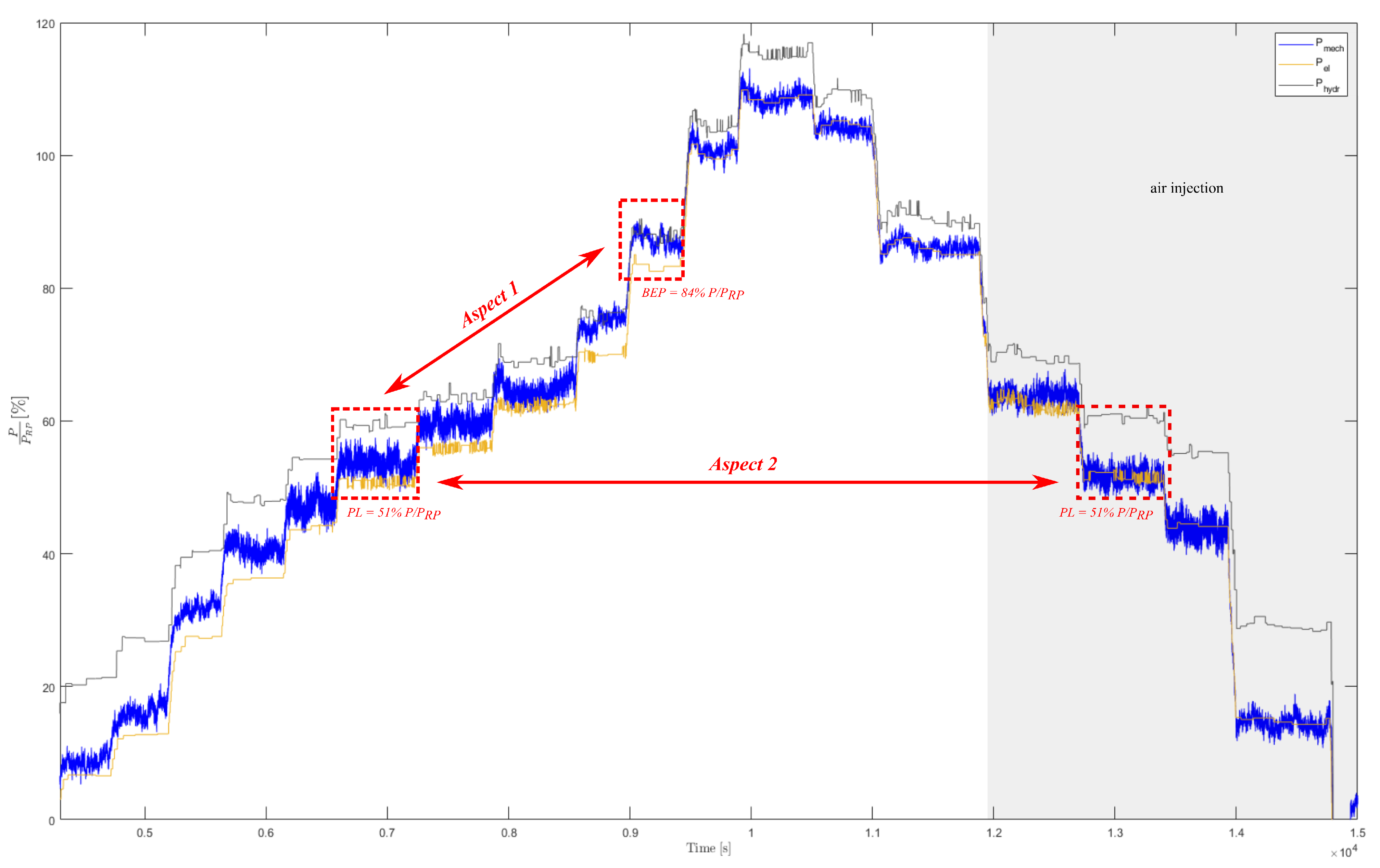
• The first aspect being compared here is the different signal behavior in the part-load range and the best efficiency point. The selection was made due to power signal behavior in Figure 4. For more detailed information, see the description.
• The second aspect apparent in this system is the injection of compressed air in the part-load range. Part-load points were measured with and without air injection during the measurement procedure. Figure 4 clearly shows this aspect. An attempt is made to quantify the effects of this air injection on the operation of the machine unit.

Figure 4 shows the measurement signals of the hydraulic, mechanical, and electrical power. The hydraulic power cannot be measured directly but is calculated and averaged from measured discharge Q and head H, the mechanical power has been determined according to Appendix A.4.6, and the electrical power has been taken from the operational data acquisition. The figure gives an impression about the time signal behavior at different load steps of the measurement procedure (see Figure 3 and description in Section 2.2). It shows that at very low loads, the hydraulic power correlates very weakly with the mechanical and electrical power. This is due to inaccuracies of the implemented Winter–Kennedy measurement for determining turbine discharge Q. Furthermore, a torque fluctuation can also be detected at this load range, which, however, does not seem to have a significant effect on the electrical power. This circumstance changes in the part load range of approximately 50–60%, where larger torque fluctuations become visible and power swinging of the generated electrical power occurs. As expected, the fluctuations are reduced again at the best efficiency and design point.

Figure 4. Time signals of hydraulic, mechanical, and electrical power.

Figure 4. Time signals of hydraulic, mechanical, and electrical power.

In the context of aspect one, the load points of ($PL=51\%P/P_{RP}$) and ($BEP=84\%P/P_{RP}$) were defined and used for further evaluations. The second aspect to be discussed within the scope of this evaluation can be observed in Figure 4 on the right-hand side of the measurement procedure, where compressed air was injected into the turbine at an operating point of approximately 60% downwards in the area of the vaneless space. Some effects of this operation mode have already been presented in [29]. This paper attempts to illustrate and discuss the changes in operating conditions caused by the injection of compressed air within the measurement signals. Therefore, a distinction is made between UP and DOWN at the operating point ($PL=51\%P/P_{RP}$). UP is operated without compressed air and DOWN with.

3.1. Examination of Measurements (Aspect 1)

Since this part deals with determining the lifetime of a Francis turbine from prototype measurement data, the consideration of the component metrological data is of primary importance. In this case, the essential information can be obtained from the temporary sensors (strain gauges and accelerometer in the hub) since those sensors were installed directly on the runner. The behavior of the strain gauges during the load tests is shown in Figure 5. Furthermore, clearly visible is that the dynamic parts of the strain signals in the part-load regions are greater than those in the best efficiency point. Figure 5 shows the raw data obtained by the strain gauges located at the pressure side of the runner blade. More about the preliminary calculations and the positioning can be found in Appendix A.3.1 and in [30].

Looking at the starting point of the strain signals in Figure 5, the refilling of the Francis turbine with cold water can be recognized. The strain gauges contract due to the temperature difference and obtain negative values, which are then used as a base for the starting sequence of the machine unit. The influence of start-ups is visible as high peaks in strains. Those transients will be investigated separately. After the SNL section, where the strain gauges at the shroud show a rising and those on the hub a more negative value, the strains change over the load steps. Hub strain gauges increase in value, whereas shroud ones decrease up to the maximum load. The strain values show the same behavior on the way down before load raising. The influence of air injection is not markable. From this point of view, it is challenging to justify air injection.

At the end of the measurement procedure, one can recognize that the strain values cannot fully recover. This means that during the measurement time, the strain gauges drift in their absolute values, having many different reasons. Those will be discussed in PART IV of this paper series. At the moment, this drift has to be considered and corrected at the conversion from strain to stress values.

Considering the theory from PART I, where individual flow phenomena were correlated in (PL and BEP) load-steps, it makes sense to identify the known frequencies within the measured data signals. For this purpose, specific signals were investigated in both the time and frequency domains. Those sensors that were temporarily mounted to the existing equipment are of particular interest. Since this group of sensors is available for inclusion as permanent sensors, they are used and evaluated here as reference sensors. Thus, the reasonableness of the sensor application is verified, and the data quality is checked. This is done by using sensor numbers 22 ($p_{con.3}$) and 26 ($a_{TH{B}_y}$) from Table 1. Sensor number 29 ($P_{mech}$) has already been used as argumentation support in Figure 5.

When studying the signal fluctuations in the PL range, one will consider the presence of a DTV. The known DTV frequency is below the rotational frequency and is expected in the following signals.

The pressure signal of the second piezoresistive transducer $p_{con.3}$ is shown in Figure 6. On the left side, the machine is operating at the best efficiency point. One can see the signal in the time domain for 30 s. The pressure fluctuations are approximately ten times lower compared to the right side, where the machine operates in the part-load region.

Similar behavior can be observed in the frequency spectrum. The amplitudes at PL are also much higher than in the BEP. In addition, frequencies below the Francis runner rotational frequency of 7.14 $\mathrm{Hz}$ become visible. A DTV frequency of around 1.4 $\mathrm{Hz}$ is expected and detectable. Furthermore, some partial frequencies of 1.4 $\mathrm{Hz}$ can be identified, which are indicative of a split DTV and not a single one.

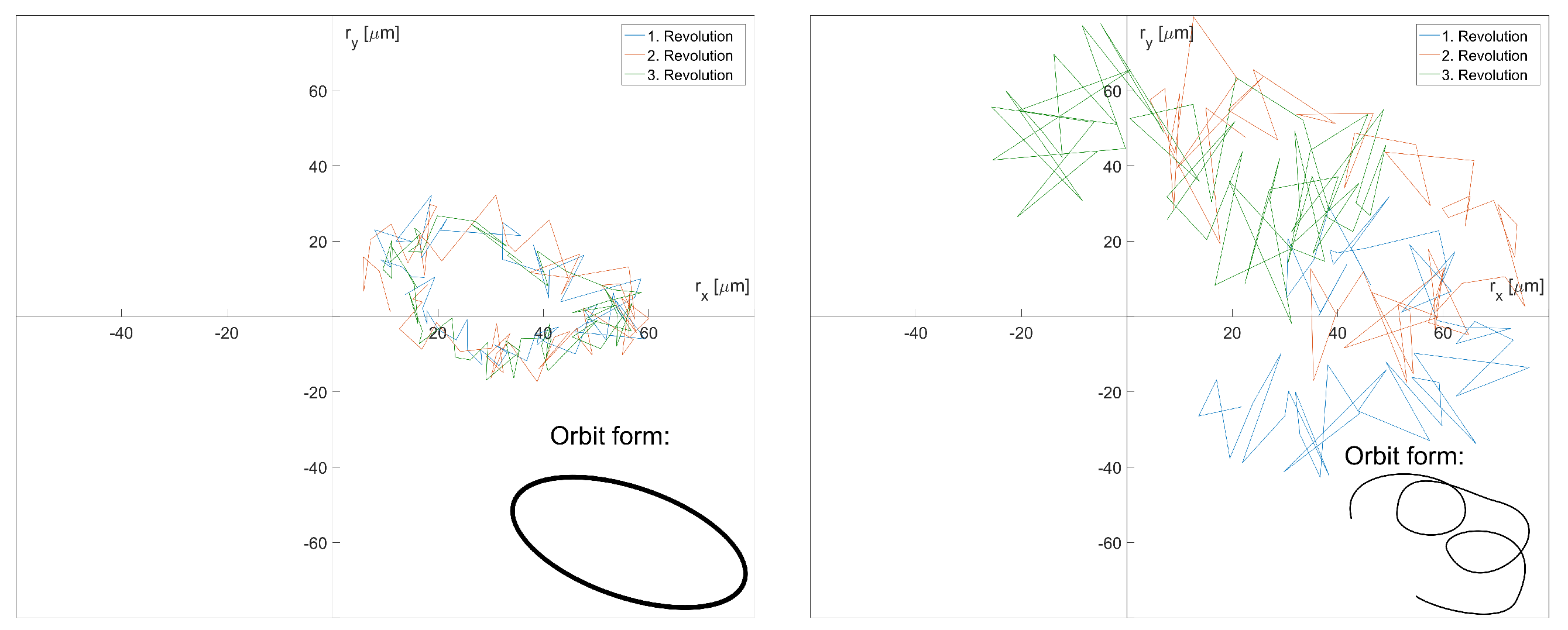
Another exciting aspect of the data analysis is the question of the effect of the DTV. As shown in Figure 4, the torque also fluctuates at this part-load point (PL), not just the hydraulic power. Accordingly, the influence on the orbit of the turbine shaft has to be discussed. The orbit represents the behaviour of the turbine shaft in the bearing quite well and is, therefore, important for determining proper concentricity.

Figure 7 shows the behavior of the turbine shaft in the area of the turbine bearing in both BEP (left) and PL (right). The orbit shape is shown for three revolutions. The BEP shows a conformal behavior of the turbine shaft and an oval orbit shape. This shape corresponds to the expectations at this load point. In the PL area, a different orbit behavior can be seen. Here, the turbine shaft is subject to specific radial forces in the bearing, which prevent an oval orbit shape. It is also subject to more significant deflection fluctuations, as seen from the $r_x$ in $\left[\mathsf{\mu }\mathrm{m}\right]$ and $r_y$ in $\left[\mathsf{\mu }\mathrm{m}\right]$ measurement signals.

Figure 6 shows the time and frequency domain of a pressure transducer measuring the flow and according phenomena with their pressure pulsations acting on the rotating and stationary part of the machine unit. Figure 7 shows the resulting behavior of the turbine shaft at the rotating reference system. The next signal to consider is the turbine casing, as this sensor is applied at the absolute reference system and showcases the machine supporting system.

Figure 7. Turbine shaft orbits at best-efficiency point (BEP) (left) and part-load (PL) point (right).

Figure 7. Turbine shaft orbits at best-efficiency point (BEP) (left) and part-load (PL) point (right).

The absolute turbine bearing vibration $a_{TH{B}_y}$ shows a significant difference depending on the operating point. For example, in the part-load (PL) point, the vibration is more than three times higher compared to the best efficiency point, as shown in Figure 8.

Additionally, one can see the appearance of higher frequencies, whereas the expected lower DTV frequencies are missing. This leads to the conclusion that the DTV and resulting pressure fluctuations are detectable at those sensors directly attached to the fluid or rotating machine unit domain. Accordingly, the DTV does not affect the turbine bearing and subsequential attachment. At PL, we see frequencies in the 230–250 $\mathrm{Hz}$ range, which could originate from the VOS. Nevertheless, that has to be proofed separately and possibly detected by correlating other sensor signals.

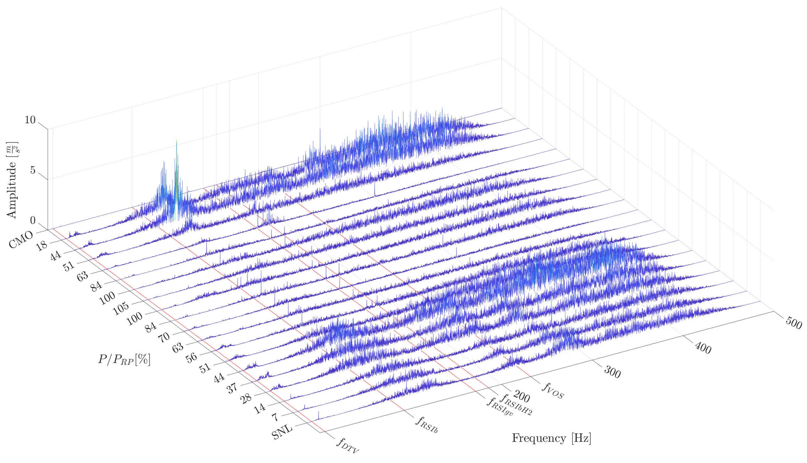
Another interesting sensor that links the flow domain with the rotating part of the machine unit is the acceleration sensor $a_{Hub}$ in $[\mathrm{m}/{\mathrm{s}}^2]$. That one is installed in the runner hub. This sensor provides acceleration values in the longitudinal axis of the turbine shaft and helps determine RSI, DTV, and VOS frequencies. Figure 9 shows a waterfall diagram of this sensor at all load levels and a frequency range of 0–500 $\mathrm{Hz}$.

The waterfall diagram shows some RSI frequencies, including harmonics. In addition, other frequency bands in the upper-frequency range are visible. The diagram also shows the load points where compressed air was injected into the machine. The PL points 63%, 51%, 44%, and 18% before the CMO are those operating points which, according to Figure 4, are in the range of compressed air injection. The injection is intended to stabilize the machine’s behaviour and to prevent undesirable flow phenomena. However, one can see that in the range of approximately $125\mathrm{Hz}$ in the PL load points 44% and 18%, a flow phenomenon must be amplified because, at the same PL load points without compressed air injection, the amplitudes of this frequency band are much lower.

Table 2. List of known frequencies and their harmonics, adapted from [31].

Phenomena	Frequency and Harmonics
Draft Tube Vortex (DTV)	1.4 Hz, 2.8 Hz, 3.2 Hz, 4.6 Hz, 6 Hz
Rotating Frequency	7.14 Hz, 14.28 Hz, 21.42 Hz, 28.56 Hz, 35.7 Hz, 42.84 Hz
Grid Frequency	50 Hz, 100 Hz, 150 Hz, 200 Hz, 250 Hz, 300 Hz, 600 Hz
Blade Passing Frequency (RSIb)	92 Hz, 185 Hz, 277 Hz
Guide Vane Passing Frequency (RSIgv)	171 Hz, 342 Hz, 513 Hz
Vortex Shedding (VOS)	232 Hz, 464 Hz, 696 Hz, 928 Hz

summarizes the frequencies, according to FIGURE 8 of PART I [1], which have been detected from the prototype measurements.

3.2. Correlation of Signals (Aspect 2)

As already mentioned in Section 2.2 and the description of Figure 9, compressed air was injected during the measurement from the overload range to the minimum load point. Looking at the part load range of 50–60% of the machine where stabilizing air was injected, the same performance fluctuations can be observed without compressed air (see Table 3, where $P_{hydr}$, $P_{mech}$, and $P_{el}$ are correlated at different load steps and with/without air injection). This leads to the assumption that the injected air through the turbine cover does not sufficiently suppress the part load draft tube vortex rope in this particular case of machine design. This assumption is also confirmed by considering the Fast-Fourier-Transformations (FFT) in Table 3. A DTV frequency of 1.4–1.5 $\mathrm{Hz}$ was detected in both directions, the PL-up and PL-down load points. This frequency indicates the presence of a DTV in this load region. 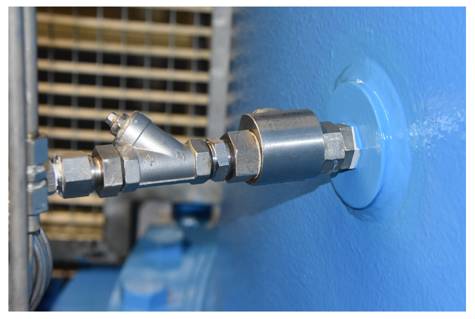This frequency was also observed in Figure 6. However, this frequency does not appear in the BEP, which is consistent with the theory. Surprisingly, the amplitude in the PL-down (with stabilizing air) is higher than in the PL-up (without stabilizing air), just as if injecting air would intensify this effect. Designs of other machine setups where the air injection is, for example, realized through the hub could lead to a different behavior. Thus, the position of air admission plays an important role in the calculation of the fatigue strength and the subsequent determination of the remaining lifetime of the runner. If the damaging loads do not decrease due to the admission of air, the runner will remain fatigued, which has far-reaching consequences in the assessment process.

Since the air is injected through the turbine cover, a dynamic pressure sensor at this point would be an advantage. A time signal with higher resolution at this point of the machine would help to calibrate the numerical flow simulation more precisely in order to better understand the underlying two-phase flow phenomenon. In the future, an application of a dynamic pressure sensor at this point should be planned for new machine sets. The problem with existing machine sets is the difficulty of instrumentation due to space restrictions.

Table 3. Time and frequency domain of PL and BEP load steps, Up–without air injection, Down–with air injection.

Sensor	PL Up (51% $\mathit{P}/{\mathit{P}}_{\mathbf{RP}}$)	BEP (84% $\mathit{P}/{\mathit{P}}_{\mathbf{RP}}$)	PL Down (51% $\mathit{P}/{\mathit{P}}_{\mathbf{RP}}$)
Power signals
$P_{hydr},$$P_{mech},$$P_{el}$
$P_{mech}$

Table 3. Time and frequency domain of PL and BEP load steps, Up–without air injection, Down–with air injection.

Sensor	PL Up (51% $\mathit{P}/{\mathit{P}}_{\mathbf{RP}}$)	BEP (84% $\mathit{P}/{\mathit{P}}_{\mathbf{RP}}$)	PL Down (51% $\mathit{P}/{\mathit{P}}_{\mathbf{RP}}$)
Power signals
$P_{hydr},$$P_{mech},$$P_{el}$
$P_{mech}$

Based on the above findings,

Table 4. Correlation of selected parameters.

Sensor	PL Up (51% $\mathit{P}/{\mathit{P}}_{\mathbf{RP}}$)	BEP (84% $\mathit{P}/{\mathit{P}}_{\mathbf{RP}}$)	PL Down (51% $\mathit{P}/{\mathit{P}}_{\mathbf{RP}}$)
$p_{TCV}$
$r_{TH{B}_x}$
Temporary data
$a_{TH{B}_{x,acc}}$
$a_{Hub}$
$S_2$

compares representative measurement signals in order to understand the machine behavior at different operating points. The time signals of the PL points ($51\%P/P_{RP}$) are compared with those at the BEP ($84\%P/P_{RP}$), where the dynamic loads on the machine should be the lowest. The interpretation of the entire machine set can be conducted from two different points of view, namely the perspective of the absolute and relative system. In the absolute system, all components are subsumed that are stationary and not rotating, e.g., the bearing, the turbine cover or generator stator, while in the relative system, the rotating components, e.g., the runner, the shaft or the generator rotor are conducted. When correlating measurement signals, it will be important to distinguish whether the used sensors contribute to one or the other system. According to Table 4, the sensors for the signals $r_{TH{B}_x}$, $a_{Hub}$, and $S_2$ are assigned to the relative system, while the remaining sensors for the signals $p_{TCV}$ and $a_{TH{B}_{x,acc}}$ contribute to the absolute system.

Correlating now the time signals of Table 4, one can see on a first shoot that the part load operation ($51\%P/P_{RP}$) is much more harmful than the operation at the best efficiency point ($84\%P/P_{RP}$). This obvious fact gets best visible when looking at the accelerometers either at the hub $a_{Hub}$ or at the bearing $a_{TH{B}_{x,acc}}$. Both show higher amplitudes at the PL area than at the BEP point. The strain gauge $S_2$ shows the same tendency as well. The future question of evaluation is the degree of damage of all operational points to the overall lifetime assessment. Furthermore, the second step is to interpret the damage by investigating monitoring sensors that are permanently applied instead of temporary measurements. Therefore, this table was divided into measures for an absolute and relative system and permanently and temporarily installed sensors. At the temporary data, one can see tendencies, which indicate the effects of the rough part load operation compared to the best efficiency point. The same tendency shows the permanently installed sensor and both signals will be correlated in further publications to obtain the proper assessment model for the investigated part.

A brief example of such an investigation would be the question of air admission affecting the energy conversion and machine behavior. As already mentioned above, the injection position plays a big issue at the machine unit investigation. Comparing the time signals of $51\%P/P_{RP}$ (PL up—without air) and $51\%P/P_{RP}$ (PL down—with air), one could detect the following: in the absolute reference system, the signal amplitude is reduced significantly, which can be observed at sensor $a_{TH{B}_{x,acc}}$, whereas in the relative reference system, the attached sensors show the same behavior. A global interpretation of this correlation would lead to the resulting formulation—at the investigated machine setup, the injected air reduces the casing vibration of the turbine bearing, resulting in a longer lifetime, whereas the rotating parts see the same load and last shorter.

Suppose we correlate the number of recorded signals with the flow phenomena one wants to detect. In that case, we obtain a first matrix (see

Table 5. Frequencies of DTV, speed, grid frequency, RSI and VOS, adapted from [31].

Phenomena	${\mathit{a}}_{{\mathbf{THB}}_{\mathit{x}}}$	${\mathit{a}}_{{\mathbf{THB}}_{\mathit{y}}}$	${\mathit{a}}_{\mathbf{GV},1}$	${\mathit{p}}_{\mathbf{con}.1}$	${\mathit{p}}_{\mathbf{con}.3}$	${\mathit{a}}_{\mathbf{con}}$	$\mathbf{DMS}-\mathit{D}2$	$\mathbf{DMS}-\mathit{S}2$	${\mathit{a}}_{\mathbf{Hub}}$
Draft Tube Vortex (DTV)				X	X		X	X	X
Rotating Frequency	X	X		X	X		X	X	X
Grid Frequency	X	X		X	X				X
Blade Passing Frequency (RSIb)	X	X	X	X	X	X			X
Guide Vane Passing Frequency (RSIgv)	X	X	X	X	X	X	X	X	X
Vortex Shedding (VOS)	X	X	X	X	X	X			X
Sensor group	Perm. MD		Temporary Validation				Temporary Assessment
MD syst. upgrade	o	o	+ +	+	+	+ +	- -	- -	- -

o = neutral, as already installed, + = positive, + + = extremly positive, - - = not suitable.

) that can be used for further considerations in machine diagnosis.

Table 5 contains sensors of the different groups from Table 1 and indicates which sensor can be used to detect flow phenomena. In addition, a classification has been made as to which sensor seems most suitable for a machine diagnostics upgrade. $a_{TH{B}_x}$ and $a_{TH{B}_y}$ are already installed in this hydropower plant and serve, therefore, as a base. Acceleration sensors $a_{GV,1}$ and $a_{con}$ mounted outside of the machine have the highest potential to be included in a machine diagnosis setup. The installation is rather easy and the sensor lifetime is according to industrial standard. Pressure transducers such as $p_{con.1}$ and $p_{con.3}$ have a good potential from the data quality but lower opportunities to be included in a machine diagnosis system due to the sensor lifetime. Sensors such as $DMS-D2$, $DMS-S2$, or $a_{Hub}$ deliver the most accurate data, but have a limited lifetime and are, therefore, not suitable to be included in a permanent machine diagnosis system.

3.3. Lifetime Determination by Using Strain Gauges

During the measurement, the stresses occurring at the strain gauge positions over the entire operating range of the system were recorded. Similar to what was already shown in PART II [2], the static and dynamic stress components, as well as the damage factors and the resulting values of the lifetime at the strain gauge positions, were evaluated using the measured stress signal. The methodology used for this has already been explained in detail in PART II [2]. Results for selected strain gauges and operating points can be seen in [30]. A description of the stress evaluation and corresponding procedure is already published in [30,32].

3.3.1. Stress Evaluationat the Position of Strain Gauges

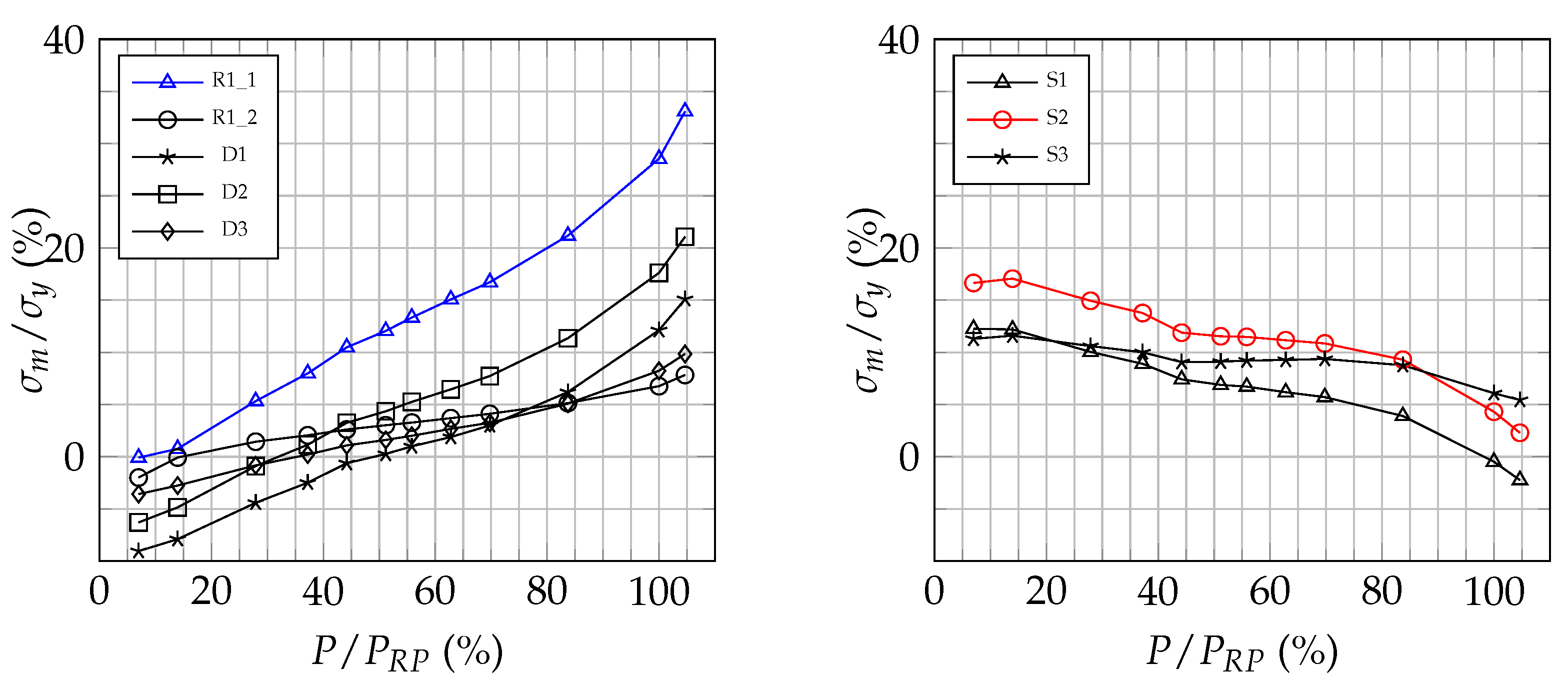
Static Stress Results

Figure 10 and Figure 11 show the static mean stress ${\sigma }_m$, defined as the arithmetic mean value of the measured signal at the suction and pressure side transitions from blade to hub and shroud on the trailing edge. The results are normalized by the yield strength ${\sigma }_y$ of the runner material X5CrNi14-3 received from a test report of the Fraunhofer Institute [33].

At the transition of the runner blade to the runner hub, significantly higher mean stresses occur on both the pressure and suction sides than at the shroud. This behavior is consistent with the numerical results from PART II [2] and has also been shown in earlier investigations of an impeller with similar specific speed $n_q$ (see [1] for the definition of $n_q$). The absolute maximum results for the first principal stress of the rosette R1-1 at overload ($105\%P/P_{RP}$), whereby even this value is still clearly below the failure-critical material parameters. Furthermore, it can be seen that with increasing power, the position of the highest measured static stress changes from the suction-side strain gauge S2 to the pressure-side placed rosette R1 in the range from (37–44% $P/P_{RP}$).

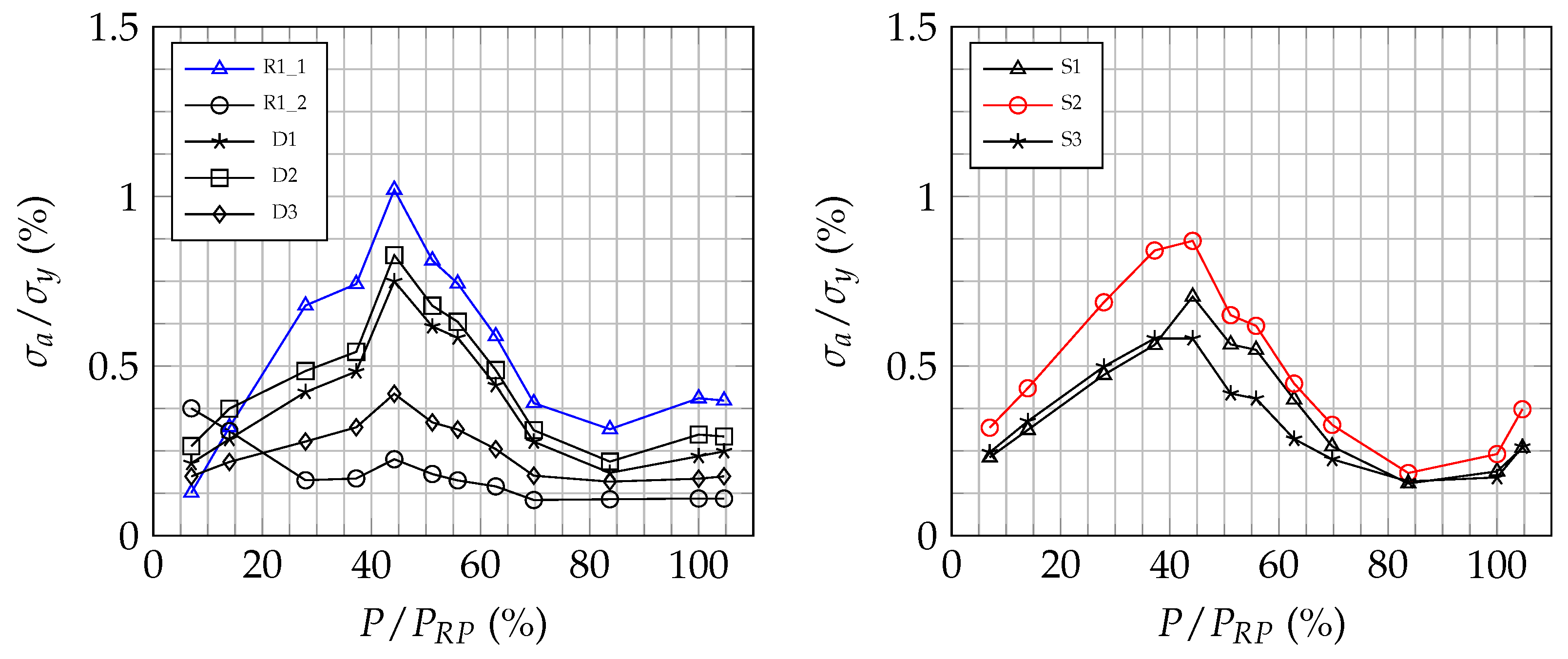
Dynamic Stress Results

To compare the dynamic stresses at different strain gauge positions throughout the whole operating range of the plant, the normalized dynamic stress values (${\sigma }_a/{\sigma }_y$) of the measured time signals are shown in Figure 12 and Figure 13.

As with the static stresses, the dynamic stress components are also significantly higher at the transition to the hub than at the shroud. The highest values are again found at the strain gauge positions R1 and S2 with the absolute maximum for R1 at ($44\%P/P_{RP}$). In general, it is easy to see that the amplitudes near the RP and BEP are lower than at the remaining operating points. Towards lower power, there is a significant increase in dynamic stresses for all strain gauges with the maxima between (37–44% $P/P_{RP}$). At the deep part load, these effects then decrease again. This behavior indicates that partial load vortexes occur in the range of (37–44% $P/P_{RP}$), which mainly attach themselves to the runner hub and cause increased dynamic stresses.

3.3.2. Stress Concentration Factor (k-Factor Concept)

Stress concentration factors are used to evaluate the maximum stress intensity points (hotspots) from a nominal stress point. The entire concept has already been discussed in SECTION 3.3.1 in PART I [1] and should not be repeated here. In summary, there are two challenges to cover: the shifting hotspot at each load step of the turbine and the unknown multiplication factor for the notch influence, as a Francis runner is no simple construction part. The consequence is that the k-factor concept is not applicable on this kind of construction.

3.3.3. Analytical Strength Assessment

According to [34], the analytical strength assessment can calculate the fatigue strength of simple or welded steel components. This analysis can either be performed with nominal stresses using k-factors or local stresses. The problem of stress intensity factors has already been discussed above and in detail in SECTION 3.3.1 in PART I [1]. The present design of a Francis runner and the variability of the hotspot at different load steps make using k-factors "de facto" impossible. Therefore, it is necessary to use the method of local stresses in an analytical strength assessment according to [34]. However, a closer look at this alternative also shows that design factors are required to evaluate form factors and notches. The authors also believe this analysis is not target-oriented and can only be conducted with further stress calculations using FE methods.

Therefore, according to Figure 1, the new method was developed, and an analytical strength assessment according to [34] was omitted. The prototype measurements and evaluations of the signals serve to validate the simulation. Stress analyzes are only carried out at those points that can be unambiguously assigned and correspond precisely to the numerical simulation. They give a first impression of the existing mechanical stresses in the runner and serve as a basis for further correction factors derived from the difference between computation and experiment.

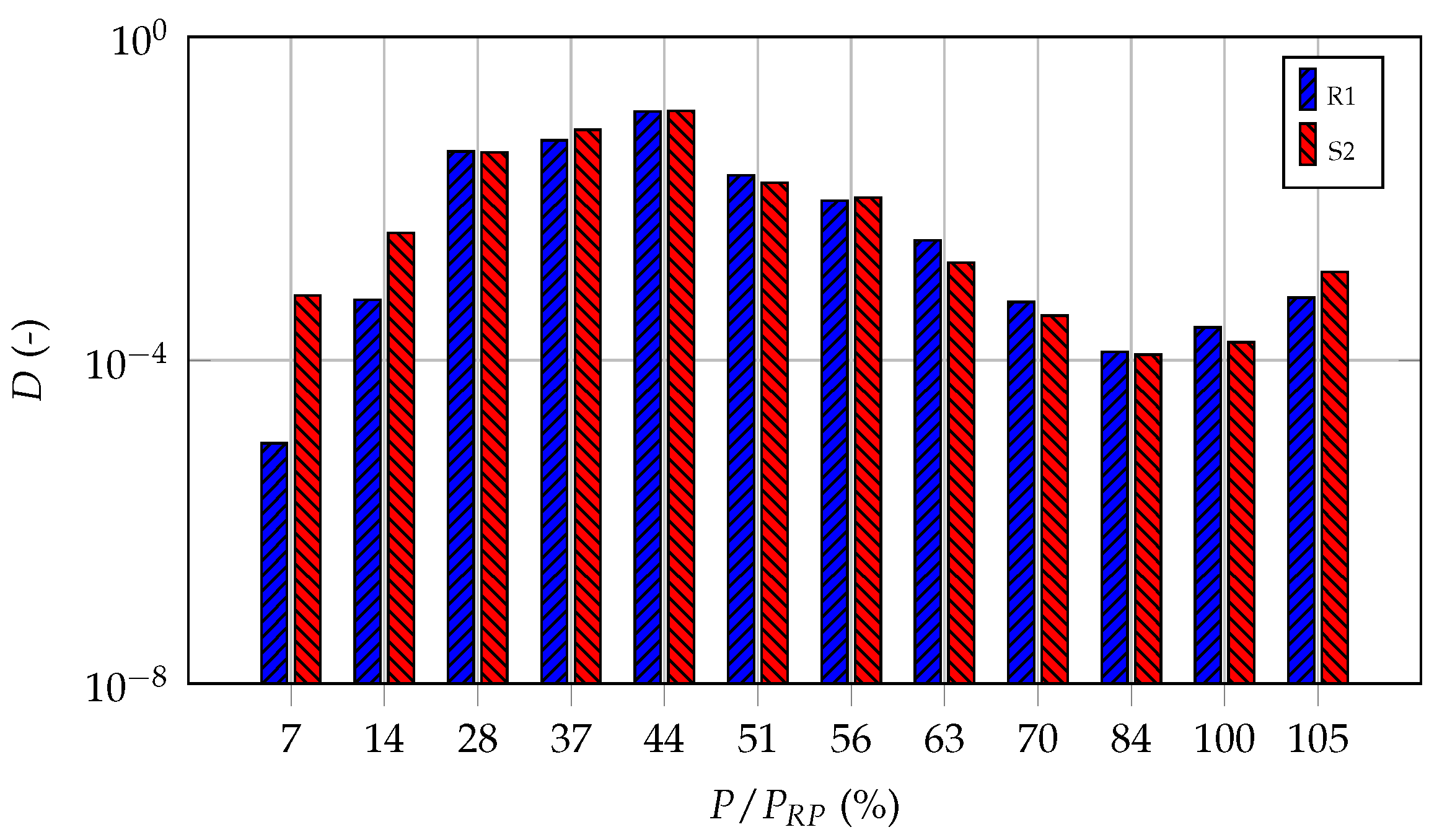
3.3.4. Damage Factors

The load spectrum obtained from the measured data by means of RFC is compared with the SN-curve of the runner material to determine the damage. As already described in PART II and applied in [30,32,35] and other publications, the modified damage hypothesis “Miner Elementar” according to Palmgren and Miner [36] is used. As can be seen from the static and dynamic stress evaluations, R1 and S2 are the failure-critical strain gauge positions. For this reason, the associated damage factors were determined only for these two strain gauges.

As Figure 14 shows, the damage level is decreasing towards the BEP and RP for both strain gauges. Except for ($7\%P/P_{RP}$), the rosette R1 shows a lower damage factor. These results correspond to the behavior of the dynamic stresses shown in Figure 12 and Figure 13, where the values are smallest at the same operating points. Going down further in part load, a continuous increase of the damage can be observed with the maximum value at ($44\%P/P_{RP}$) for R1 and S2, where also the highest stress amplitudes occur. In deep part-load, the values are decreasing again.

3.3.5. Lifetime Prediction at the Position of Strain Gauges

However, in order to be able to make actual statements about the fatigue and further the lifetime of the Francis runner, the damage factors shown are not sufficient. The knowledge of a corresponding load spectrum of the plant is necessary. For this purpose, as already in PART II, the fictitious operating times of the two load scenarios base load and grid stabilization published in PART I [1] (see FIGURE 5, p. 7) were used. The values of the service life determined from the measured stresses with the aid of the two load scenarios are shown in

Table 6. Expected lifetime for R1 and S2 in years for base load and grid stabilization.

Position	Base Load [Years]	Grid Stabilization [Years]
R1	2386.2	45
S2	2082.5	43.2

.

Although the damage factors in the partial load are slightly higher for R1, the position of the S2 strain gauge turns out to be critical for failure, as can be seen in Table 6, due to the weighting with the associated operating times for both scenarios. However, it should be noted that, especially for grid stabilization, there is only a small difference between the expected lifetime.

4. Discussion

Based on the above illustrations and results, the following points of discussion are of interest:

• Looking at the individual flow phenomena and measurement signals, one can see the different applicability of individual sensors. There is a specific correlation between flow phenomena and sensor application. This point was illustrated in Section 3.1 for different load points. Accordingly, it should be taken into account when correlating sensors and data. The resulting frequencies have been summarized in Table 3.
• An important result is Table 5. Within this table, one can see the possibility to detect a specific flow phenomena with different kinds of sensors. Furthermore, this table is just an excerpt of all possible sensors. The sampling rate and the sensor application location make this table so specific. This table has two particular advantages: on the one hand, the chance to add some additional sensors to the machine diagnosis system and, on the other hand, the availability to build a virtual/soft sensor detecting flow phenomena from a multi-sensor level.
• The mechanical stresses to assess the lifetime of a Francis runner can only be determined at predefined points. Depending on the selection of the points to be examined on the runner and the number of available sampling channels on the data acquisition system, either linear strain gauges or strain gauge rosettes are used. Linear strain gauges have the advantage of occupying only one recording channel but must be attached at points where a uni-axial stress gradient is expected. This usually leads to measuring points further away from the hotspot, the point with the maximum mechanical stresses. However, several linear strain gauges are often applied at these points for redundancy reasons. Suppose the hotspots are already known from previous investigations. In that case, a strain gauge rosette consisting of three linear strain gauges at different angles to each other can be applied in this area. The informative value of the stress measurement increases considerably as long as the hotspot does not change under different load influences. A suitable selection of strain gauge measuring points requires a specific experience with the fatigue assessment of Francis runners.
  This inevitably leads to the discussion of extrapolation in the direction of those points with the highest mechanical stresses, which are decisive for the fatigue strength calculation. In many technical applications, the influence of possible geometric changes, such as notches, curves, and cross-section changes, is considered in this context by introducing stress concentration factors, so-called k-factors. Since the dynamic loads are used as the design basis for the fatigue strength calculation, and these can change locally from load case to load case, the k-factors would also have to be adjusted in each calculation step to make statements that are true to reality. This is not feasible with a purely metrological approach. As a solution, either static k-factors are chosen, which can significantly distort the result, or a combination with strength calculations is carried out.

Since the locations with the maximum mechanical stresses depend on different load cases and the underlying flow phenomena, a combination of experiment and simulation is the best possible solution. Only in this way can moving hotspots be assessed more accurately and the fatigue strength calculation improved. The result is a validation system that supports measurement and numerical calculation.

5. Conclusions

The following conclusions could be drawn:

+

Additional sensors:

In the section at the vaneless space, an unsteady pressure measurement sensor would be very useful to detect pressure fluctuations, but the instrumentation is very difficult in this region and requires in existing machines a major effort if a monitoring point does not already exist. A time signal with a higher resolution at this point of the machine would help to calibrate the numerical flow simulation more precisely in order to better understand the underlying two-phase flow phenomenon.

The main part of the installed pressure gauges are chiefly used for steady static pressure measurements. For many applications, it is very important to know the pressure distribution from the inlet to the outlet of the machine. Afterward, all steady static pressure monitoring points are listed and described, starting from the turbine closing valve and then in flow direction through the machine, ending at the draft tube outlet, as shown in Figure 2.

In the future, an application of a dynamic pressure sensor at this point should be planned for new machine sets. The problem regarding existing machine sets is the difficulty of instrumentation due to space restrictions.

+

K-factor concept versus local mechanical stresses:

The main point is that one cannot investigate the hotspots with measurements. Significantly, if the hotspots vary, meaningful measurements are not possible. Such investigations are performed because stresses are measured at the points where known conditions are expected; moreover, an extrapolation takes part.

+

Need for numerical calculation with validation through measurements:

Taking previous conclusions into account, the way to perform better and newer fatigue evaluations is a combination between numerical simulations and measurements. Numerical simulations can give us a better insight according to the maximum stresses but should be validated by precise measurements.

+

Virtual/soft sensor:

The current results conclude the possibility of developing a virtual/soft sensor. This combines several physical sensors to detect certain flow phenomena better and limit them in the characteristic operating field. This topic will be displayed in Part IV of this paper series.