Abstract
This paper presents an alternative methodology to obtain the precise amount of shunt reactive power compensation in order to simultaneously reduce the total reactive power losses, improve the voltage profile and increase the loading margin of power systems. The amount of shunt reactive power compensation to be allocated is determined based on the curve of the total reactive power losses versus the voltage magnitude of a chosen bus. The best places for shunt reactive compensation are defined by the load bus participation factors of the critical mode provided by the static modal analysis. Simulation results employing shunt capacitors obtained with the new approach for the IEEE test systems (14, 57 and 300 buses) show that the procedure leads to a reduction in total reactive and active power losses and simultaneously improves the voltage profile and loading margin.
1. Introduction
The steady-state voltage stability analysis aims to identify how close the power system is to its operational limit, the critical buses and areas prone to voltage collapse. It also seeks to define the necessary reinforcement actions to improve the voltage stability margin. In these analyses, it is common for the joint use of static methods such as P-V and V-Q analyses associated with the steady-state modal analysis applied to the reduced Jacobian matrix [1,2,3,4,5,6,7,8,9,10,11,12,13].
The P-V analysis is used to obtain a power system’s maximum loading point (MLP), i.e., the maximum additional load that the system can supply starting from a base case [8,9]. Next, it must be verified if the power system margin meets the values recommended by the electric sector. According to the Western System Coordinating Council (WSCC), its member utilities must have at least a 5% P-V margin under any single-element contingency [6,7]. If the recommendation is not met, the type, location and size of appropriate reinforcement must be identified to prevent voltage instability. In such cases, the steady-state modal analysis has been used since it allows us to infer whether the electric power system is operating near the voltage collapse point and identify which areas are more prone to voltage instability so that corrective measures are taken [14,15]. Setting the best placement and amount of the reactive power source is very important in today’s electricity market. The steady-state modal analysis has been applied to assist in solving the problem of the allocation of reactive power sources in the electric power network. In contrast, the Q-V analysis determines the reactive power margin and the amount of the shunt reactive power compensation source on specific buses. The most common and less expensive kind of shunt reactive power compensation is the shunt capacitive compensation. Its use has several benefits, such as an increased loading margin and decreased active and reactive transmission losses. The transmission losses involve high capital costs since they represent 5 to 10% of the total generation [16]. These losses can significantly increase with the load increase, usually accompanied by a deterioration in the voltage profile [17]. The reactive power loss reduction involves direct economic gain due to the reduction in the active power losses and, thus, a lower production cost. Moreover, with the increased availability of reactive power, a larger steady-state voltage stability margin and an improved voltage profile can be obtained. The load bus participation factor values provided by the modal analysis indicate the best places (buses) for shunt reactive power compensation since they associate the variation in reactive power with voltage variation [14,15,18,19,20].
The amount of reactive power compensation needed to take the system to a secure operating point is determined by the V-Q curve, which is obtained by adding a fictitious synchronous condenser at the chosen bus, converting it from the PQ to the PV type with infinite reactive capability [8,9,14]. For the selected bus, the reactive power outputs are obtained by solving a power flow for each voltage magnitude value specified. For a given loading condition, the reactive power margin (RPM) available at the bus is computed by the difference between the zero reactive power output of the synchronous condenser (the current operating point) and its value at the bottom of the V-Q curve. The RPM decreases as the load increases, and the condition of maximum active power transfer without reactive compensation occurs when the V-Q curve is tangent to the horizontal axis (V axis); the system is at the critical level. Several procedures have been proposed to improve the steady-state voltage stability margin using off-line and on-line redispatching of the reactive power injection of generators, the allocation and setting of reactive power sources, and in emergencies, the load shedding strategies [18,19,20,21,22]. In [18], the reactive injection from generators and synchronous condensers is rescheduled to improve the voltage stability margin. The method uses the active participation factors given by the modal analysis technique to define penalty factors for Var sources incorporated into the optimal power flow (OPF) formulation. In [19], the voltage stability margin is indirectly increased using participation factors derived from the critical eigenvectors of the Jacobian matrix at the MLP. The redispatch process involves taking actions based on the modal participation factors calculated for generator and load buses. To supply generators that have a negative impact on the system margin, as indicated by the modal index, these generators receive high costs in the objective function of the optimal power flow (OPF) program utilized during the redispatch process. In [20], the voltage stability margin is improved through reactive power rescheduling. The reactive power of generators is increased or decreased by adding penalty terms to the optimal power flow objective function according to ranking coefficients obtained using modal analysis. The method has been simulated using both coefficients, the reactive index (for all generators) and active index (for all generators except for the slack bus), as ranking coefficients.
Numerous algorithms have been proposed to optimize distributed generators’ placement and size to reduce power system losses and improve voltage profiles [23]. These algorithms aim to enhance the efficiency and reliability of power systems by strategically determining the most suitable locations and capacities for distributed generation (DG). However, they are still subject to several limitations. In [23], a reconfiguration methodology was introduced utilizing a hybrid optimization algorithm that combined the genetic algorithm with the improved particle swarm optimization algorithm. This methodology aimed to minimize active power loss while maintaining the voltage magnitude at approximately 1 pu. Simulation results demonstrated the effectiveness and promise of this approach in optimizing network reconfiguration problems, yielding an average reduction in real power loss of 40%.
In [21], an OPF is used to make a redispatch of the active/reactive power injection of generators. During the proposed procedure’s application, the generators and shunt capacitor participation factors are obtained by modal analysis for each new operating point. Units with a negative impact on loading margin are penalized with high costs and considered in the objective function of the OPF.
Several other methods using the multi-objective approach for the optimum shunt reactive power compensators’ placement and sizing have also been reported in the literature [24,25,26,27,28,29]. FACTS devices, DG and shunt capacitors are frequently considered for these methods. Reducing power system losses, improving the voltage profile and increasing system voltage stability are common goals in a multi-criterion objective function. To reduce the starting point dependence, evolutionary techniques have been applied to solve the optimal power flow problem. A nonlinear equality and inequality constrained multi-objective optimization problem has been proposed in [24]. A new evolutionary technique, bacteria foraging, solves the optimization problem. Real power loss minimization and voltage stability limit maximization are considered in the objective function to obtain the transformer tap values, the location, and both the magnitude and phase angle of the series injected voltage of a unified power flow controller. A solution procedure based on particle swarm optimization (PSO) for determining the optimal location and size of shunt devices was proposed in [25], aiming at increasing the system voltage stability margin while maintaining an acceptable voltage profile. PSO was also used to determine the most sensitive buses to be candidates for the shunt devices’ installation. In [26], PSO was used to solve the multi-objective function, considering the minimization of power losses and the maximization of bus and line transmission voltage stability for optimal DG placement and sizing. Stability indexes were used to find the power system’s weakest voltage bus and transmission line. In [27], the optimal location and size of shunt reactive compensators were obtained using a metaheuristic optimization technique to enhance the voltage stability, improve the voltage profile and minimize the power loss while minimizing the total cost. First, the suitable buses were identified by the modal analysis method and then used by the algorithm to determine the optimal sizing of shunt compensators. A total voltage stability index for overall stability assessment, used as the objective function for optimizing the settings of compensation devices, was proposed in [28]. A hybrid differential evolution algorithm was used to solve the optimization problem of voltage stability enhancement, reduce the line losses, and determine the locations and sizes of shunt reactive compensators, the tap settings of on-load tap changing (OLTC) transformers, and excitation settings of synchronous condensers. A new overall voltage stability index was proposed in [29] to improve the voltage stability margin. The optimal size and location of DG units were determined by defining an objective function to minimize active power losses and maximize the proposed index. To solve the optimization problem, an imperialistic competitive algorithm method was used. In [30], a novel approach was introduced to reduce the total real power losses by utilizing a modified continuation power flow (MCPF) technique. An additional parameterization equation, considering the total real power losses and reactive power equations at generation buses, was incorporated into the conventional power flow equations to achieve this objective. The voltages at PV buses were treated as control variables, and a new parameter was selected to reduce the total real power losses. In contrast to the conventional power flow (CPF) method, which aims to determine P-V curves’ maximum loading point (MLP), the MCPF approach focuses on improving the loading margin by reducing real power losses through a continuation method. Unlike CPF, where the load and real power generation are increased in predefined directions, the MCPF technique maintains fixed values for these parameters.
This paper presents an alternative methodology to obtain the amount of shunt reactive power compensation. The goals are to simultaneously reduce the total reactive power losses, improve the voltage profile and increase the loading margin. The definition of the amount of shunt reactive compensation to be allocated is determined based on the curve of the total reactive power losses versus the voltage magnitude of a chosen bus. The places for shunt reactive compensation are defined by the load bus participation factors of the critical mode provided by the static modal analysis. The simulation results employing shunt capacitors obtained with the new approach for the IEEE test systems (14, 57 and 300 buses) are presented and discussed. The results show that the procedure leads to a reduction in total reactive and active power losses and, simultaneously, an improvement in the voltage profile and loading margin. Moreover, comparisons between the solutions of an OPF [31], the MCPF presented in [30] and the proposed method show that it can provide similar results for the loading margin increase. Therefore, it can be a reasonable power system voltage stability enhancement alternative.
2. Proposed Method to Obtain the Amount of Shunt Reactive Power Compensation
The V-Q approach is a steady-state method of static voltage stability analysis used to determine the reactive power margin on specific buses, generally the critical buses of a power system network. In the proposed method, the static modal analysis is realized after determining the maximum loading point (MLP), and the bus of participation factors (pfki) corresponding to the smallest eigenvalue, i.e., the critical mode, is provided. Next, the reactive power analyses are made for all the load buses indicated by the load bus participation factors. Tracing total reactive power losses versus bus voltage magnitude (V−Qloss) and total reactive power losses versus generated reactive power (Qgen−Qloss) curves is similar to that used to trace the V−Q curve. To produce the curves, the bus type is changed from PQ to PV, successive values of voltage magnitudes are specified, and the corresponding values of total reactive power losses (Qloss) and generated reactive powers (Qgen) are computed and stored. Then, both curves are traced with the stored values, as shown in Figure 1a,b (refer to Appendix A for the flowchart). To exemplify the proposed methodology and the creation of Figure 1a,b, the IEEE 14 buses test system was used. The voltage magnitudes and the generated reactive power values are represented on the abscissa axis, and the total reactive power losses (Qloss) as the ordinate. The reactive power losses are given by [32]:
where: Vk and Vm and θk and θm are the respective magnitudes and angles of the nodal voltage of bus k and m, Ω is the set of all network buses, and bkm and bkmsh the respective series susceptance and shunt charging of the line transmission between buses k and m. The generated reactive power is calculated by [9]:
where λ is the loading factor, V and θ are the respective vectors of the nodal voltage magnitudes and phase angles, and is the reactive power consumed at PV buses. For a bus k, Qk(θ,V) are given by [32]:
where NB is the number of buses of the system, Gkm and Bkm are the real and imaginary parts of the element km of the nodal admittance matrix Y = [G] + j[B], respectively.
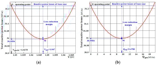
Figure 1.
(a) Total reactive power losses in the function of bus voltage magnitude (V−Qloss), (b) total reactive power losses in the function of generated shunt reactive power (Qgen−Qloss).
As shown in Figure 1a,b, the base case operating point (point “O”) corresponds to the total reactive power loss at the base case (QlossBC = 31.2162 MVar), where the generated reactive power (Qgen) is zero, which corresponds to the intersection of the curve with the ordinate axis in Figure 1b. Point M corresponds to the lowest total reactive power loss (30.9954 MVar) obtained by the reactive power compensation at the bus. The total reactive power loss reduction (RLR) is calculated by:
where: QlossCQ is the total reactive power loss at base case considering the shunt reactive power compensation. The total loss reduction (31.2162 − 30.9954 = 0.2208 MVar) corresponds to the distance from the bottom of the curve (point M) to the horizontal dashed line passing through point O. From Figure 1b it can be seen that the reactive power compensation needed is of 9.478 MVar at the voltage magnitude of 1.047 pu, this is not a fixed value, but it varies with the voltage square (Qgen =BV2). Therefore, considering the installation of a shunt capacitor bank (B) of 8.6461 MVar at a nominal voltage magnitude of 1.0 pu, a total reactive power loss reduction of 0.7073% is obtained. The load margin increase (LMG) is calculated by:
where: LMBC and LMCQ are the power system loading margin at base case without and with a shunt reactive power compensation, respectively.
3. Test Results
Intending to point out the features of the proposed methodology, numerical tests were conducted on the IEEE test systems (14, 57 and 300 buses). These systems were chosen due to their different characteristics. The IEEE-14 presents a simple topology close to a radial structure, formed by nine load buses (PQ), four generation buses (PV) and one slack bus; the IEEE-57 presents a mesh grid topology with a ring structure, with one slack bus, six PV buses and fifty PQ buses; and the IEEE-300 is a large and heavily loaded system with characteristics commonly found in natural, sizeable electric power systems, and this system presents one slack bus, sixty-eight PV buses and two hundred and thirty-one PQ buses. The reactive power generation limits of the PV buses are taken into account in all the tests. The load and generation variations occur according to the loading factor (λ). The P-V curves are traced starting from the base case (λ = 1) until very close to the MLP. A continuation power flow (CPF) using the loading factor (λ) as a parameter is used for tracing all the P-V curves [9,33,34]. The CPF is calculated by (6), with more details of this in [35]:
For (6), assume that the grid loading is proportional to the base case and consider the power factor constant. The vectors Psp and Qsp can also be defined as being equal to (kPgPgsp + kPcPcsp) and kQcQcsp, respectively. The kPg, kPc and kQc vectors are fixed parameters that characterize a specific load scenario. From the base case (λ = 1), the value of λ gradually increases until close to the MLP (due to the singularity of the Jacobian matrix). The P-V curves are traced from a given base case until a very close point to the maximum loading point (MLP). The active and reactive loads and active generation variations occur according to the loading factor λ, i.e., proportionally to their corresponding base case values [35]. The CPF method employs the local parameterization technique to eliminate the Jacobian matrix’s singularity at MLP. This involves altering the parameter in the vicinity of MLP from the loading factor (λ) to a newly selected variable. The selection of an appropriate continuation parameter depends on the variable that exhibits the highest rate of change near a specific solution. Typically, the voltage magnitude of bus k (Vk) is regarded as the parameter near MLP. Once a few points on the curve have been traversed, it reverts to λ. Note that a sign change in Δλ indicates that the MLP has just been passed, and therefore, its corresponding value in the previous point is considered the target value.
To be most effective, the modal analysis should be performed in MLP or as close to it as possible [14]. Thus, to have a more precise value of MLP for the application of modal analysis to obtain the participation factors of the critical mode, during the P-V curve tracing, a mismatch convergence threshold of 10–8 pu is adopted and a step size control method based on the normalized tangent vector is used [36]. The step size (σ) is given by , where is the Euclidean norm of the tangent vector [dθ dV dλ]T, and σ0 is a predefined scalar. The value of 0.1 was adopted for σ0 for all the analyzed systems. As the system becomes stressed, i.e., closer to the MLP, the norm of the tangent vector increases and σ decreases. To avoid the numerical difficulties that occur in the vicinity of the MLP, due to the singularity of the Jacobian matrix, the voltage magnitude with the largest variation is considered as a parameter and is now considered a dependent variable. It is important to note that the step size control method remains based on a normalized tangent vector considering λ as a parameter, and thus, the obtained operating points will always belong to the upper part of the curve but never to its lower part. The step size convergence threshold was also 10–8 pu. With this procedure, eigenvalues smaller than 10–7 are obtained for all the studied systems. To trace the curve of total reactive power losses versus the bus voltage magnitude, the mismatch convergence threshold is 10–5 pu.
3.1. Performance of the Proposed Method to Determine the Total Reactive Power Loss Reduction (RLR) of IEEE-14
Figure 2a shows the P-V curves of the IEEE-14 system considering the reactive power limits of generators (PV buses). The maximum loading points of IEEE-14 with and without the limit control of reactive power were obtained following the P-V curve tracing procedure described in Section 3. The difference between the maximum loading point (λ = 1.7444 pu) and that of the base case (λ = 1), i.e., the loading margin, is approximately 74.44%. It represents a loading margin reduction of 75.558% compared to that of the base case (λ = 4.0209 pu) without reactive power limits, highlighting the importance of reactive power availability for active power transfer.
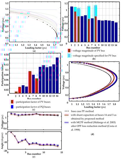
Figure 2.
IEEE-14 system with the reactive power limits of PV buses: (a) P-V curves, (b) voltage profile at MLP, (c) bus participation factor of the critical mode of JR matrix, and (d) P-V curves and (e) voltage and angle profiles obtained with loss reduction procedures: inclusion of the shunt reactive power compensation by the proposed method, and from the converged state of MCPF and OPF methods [30,31].
From the voltage profile presented in Figure 2b, it can be seen that at MLP, the smaller voltage magnitudes, in ascending order, occur for buses 14, 13, 12, 10 and 11. It can also be seen that all the reactive power limits of the four PV buses are reached since the current–voltage magnitudes (in red in Figure 2b) are smaller than the respective specified values (in cyan in Figure 2b). Thus, as shown in Table 1, at MLP, the reduced Jacobian matrix (JR) presents thirteen eigenvalues: nine from PQ buses and four from PV buses, which switch to the PQ type when their limits are violated. Figure 2c presents the respective pfki corresponding to the smallest eigenvalue (9.569 × 10⁻⁷), i.e., for the critical mode. Note that its value is an indication that the system is very close to the MLP, in which the determinant of the Jacobian matrix is zero.

Table 1.
Eigenvalues of IEEE-14 at MLP (λ = 1.7444 pu) considering the reactive power limits of PV buses.
Table 2 and Figure 2 present the simulation results for the IEEE-14 obtained by the total reactive power losses versus bus voltage magnitude curve methodology presented in Section 2, considering the reactive power limits at generator buses (PV buses). The second column of Table 2 shows the values of the participation factors of the critical mode placed in descending order along with its bus number identification that is presented in the first column. The fifth column presents the reactive power of capacitor banks (Qgen) for which the smaller total reactive power losses occur, while the other columns contain the respective values of the total active (Ploss) and reactive (Qloss) power losses, the bus voltage magnitudes at the base case (|VBC|), the loading factor and the voltage magnitudes of the critical bus (|V|), the load margin increase (LMG) computed by (5) and the total reactive power losses reduction computed by (4). As presented in the 11th column of Table 2, compared to the base case value, the largest reduction in the total reactive power loss (26.8085 − 26.4508 = 0.3577 Mvar or 1.334% by using (5)) occurs with the inclusion of a capacitor bank of 26.6529 MVar at bus 5. However, the most effective buses to make the shunt compensation aimed at reducing losses and increasing the loading margin can be seen in columns 10 and 12 of Table 2, and in Figure 3b,c. According to the results, it is verified that the most efficient buses for increasing the loading margin are the buses 9, 10, 11, 13, 12, 14 and 7, whereas for total reactive power loss reduction the most efficient are the buses 14, 13, 10, 9 and 11. These buses are also indicated by the participation factors of the critical mode as shown in Figure 3a.
Table 2.
Simulation results for the IEEE-14 obtained by the total reactive power losses versus bus voltage magnitude curve method considering the reactive power limits at PV buses (QlossBC = 26.8085 MVar; PlossBC = 13.3589 MW).
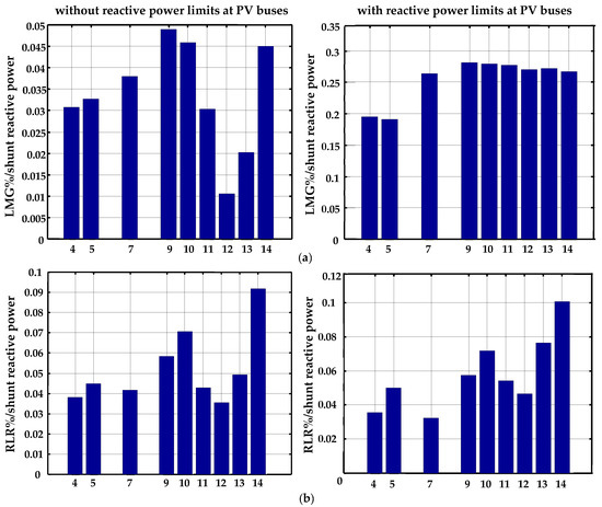
Figure 3.
Influence of reactive power (Q) limits (with and without reactive power limits at PV buses) on the performance of the proposed method for IEEE-14: (a) loading margin increase and (b) total reactive power losses reduction normalized by the shunt reactive power compensation.
Figure 2e shows the voltage and angle profiles obtained by the MCPF [30], and the OPF [31] methods, and considering the inclusion at buses 14 and 5 of the capacitor banks obtained by the proposed method, which are presented in the fifth column of Table 2. The voltage and angle profiles presented in Figure 2e show that the operating points obtained by all the methods are close to each other. Figure 2d shows the P-V curves traced by using a CPF and, as a starting point, the respective converged solution of the MCPF, the OPF and the proposed method. Their respective MLPs can be seen in the fourth column of Table 3, where a comparison between the performance of the methods is presented. By the inclusion of capacitor banks, the obtained loading margin is improved by about 7.7%, with a reactive power reserve (RPR) of 69.9 MVar in the generators (PV buses), i.e., an addition of 32.8 MVar in the base case value (37.1 MVar). Loading margin increases of 14% and 14.7% are provided starting from the respective converged solutions of the OPF and MCPF methods but at the expense of the addition of lower reactive power reserves of 17.3 MVar and 12.5 MVar, respectively.
Table 3.
Comparison between the performances of the methods for the IEEE-14.
Figure 3 compares the influence of the reactive power limits of generators (PV buses) on the performance of the proposed method. Note from Figure 3a that the values of the load margin increases obtained with shunt compensation, but without considering the reactive power limits at the PV buses, are relatively smaller than those obtained considering the limits. This shows the greatest importance that shunt compensation presents for systems with reactive power supply restrictions in the generators.
Figure 4a,b present, in percent, the respective amounts of loading margin increase (LMG) and total reactive power losses reduction (RLR) obtained when a shunt capacitor bank of 5 MVar is applied separately on each one of the load buses of IEEE-14 indicated by the participation factors, considering the reactive power limits at the PV buses. The results obtained by the proposed methodology can be validated by comparing the results presented in Figure 4a,b with those of the respective Figure 3a,b, with reactive power limits at PV buses.
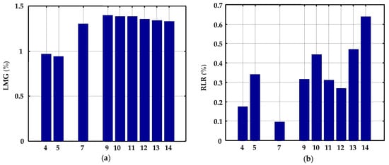
Figure 4.
Influence of 5 Mvar of shunt reactive power compensation at each load bus of IEEE-14: (a) loading margin gain, and (b) total reactive power losses reduction.
3.2. Performance of the Proposed Method to Determine the Total Reactive Power Loss Reduction (RLR) of IEEE-57
Figure 5a shows the P-V curves of the IEEE-57 system considering the reactive power limits of PV buses. The loading factor at MLP obtained by a CPF is 1.5331 pu. The total reactive and active power losses at the base case are 9.2769 MVar and 28.6127 MW, respectively. From the voltage profile at MLP presented in Figure 5b, it can be seen that the smaller voltage magnitudes occur in the vicinity of bus 31, this being the lowest. It can also be seen that, different from the IEEE-14 where all the voltage magnitudes including the PV buses are below 0.95 pu, in this system, the voltage magnitude of all load buses (in blue in the figure) is below 0.95 pu, despite the voltage magnitudes specified for the PV buses (in red in the figure) being practically attended at MLP. This voltage sag occurs mainly near the critical bus (bus 31), which can be seen (in red) in the single-line diagram of Figure 6.
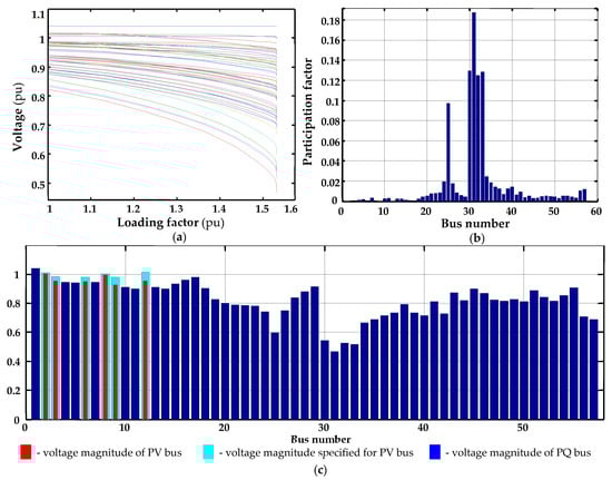
Figure 5.
IEEE-57 system with the reactive power limits of PV buses: (a) P-V curves, (b) participating factor, (c) voltage profile at MLP.
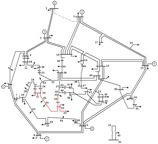
Figure 6.
Single-line diagram of IEEE-57 system, showing the vicinity of the critical bus (bus 31) affected by the voltage sag.
Table 4 shows the IEEE-57’s five lowest eigenvalues, while Table 5 shows the results obtained by the method for the buses indicated by the first ten and, aiming to compare, three of the smallest participation factors, corresponding to the lowest eigenvalue found (4.0875 × 10⁻⁸). The lowest eigenvalue indicates that the operating point corresponds to a point very close to the MLP.
Table 4.
Eigenvalues of IEEE-57 at MLP (λ = 1.5331 pu) considering the reactive power limits of PV buses.
Table 5.
Simulation results for the IEEE-57 obtained by the total reactive power losses versus bus voltage magnitude curve method considering the reactive power limits at PV buses (QlossBC = 9.2769 MVar; PlossBC = 28.6127 MW; λBC = 1.5331 pu).
The first column of Table 5 indicates the buses in the order given by the participation factors (second column). Columns 2, 10 and 12 of Table 5 and Figure 7 show the values of the participation factors, loading margin increase and total reactive power losses reduction per unit of the capacitor bank. From the analysis of these results, it concluded that the more efficient locations (buses) to perform shunt compensation in order to reduce the total reactive power losses and increase the loading margin are buses 25, 30, 32, 33 and 31. This is the same set of buses (buses physically interconnected) which belongs to the critical area identified by the participation factor indicated by the participation factors of the critical mode as shown in Figure 7a. Note from the single-line diagram of IEEE-57 that bus 25 is already installed with a capacitor bank of 5.9 MVar.
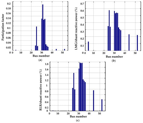
Figure 7.
Performance of the proposed method for IEEE-57: (a) bus participation factors, (b) loading margin increase and (c) total reactive power losses reduction, normalized by shunt reactive power compensation.
It should also be noted from columns 10 and 12 of Table 5 that the loading margin increase and total reactive power losses reduction are relatively larger than those of IEEE-14. Thus, the great importance that the shunt compensation has for this system can be seen, as in this case, despite the availability of reactive power in the generators, the increase in the loading margin and the loss reduction basically occurs at the expense of shunt compensation. Note also that although buses 44 and 52 are among the three with the smallest participation factors, they are also indicated by the proposed method as candidates to increase the loading margin and reduce the total reactive power losses. Figure 8b,c,e present the respective percentages of loading margin increase (LMG) and total reactive (RLR) and active (ALR) power losses reductions, obtained with a shunt capacitor bank of 10 MVar applied separately at each one of the load buses indicated in the first column of Table 5. Compared with those presented in Figure 7 and Figure 8c, the coherence of the results provided by the analysis can be confirmed.
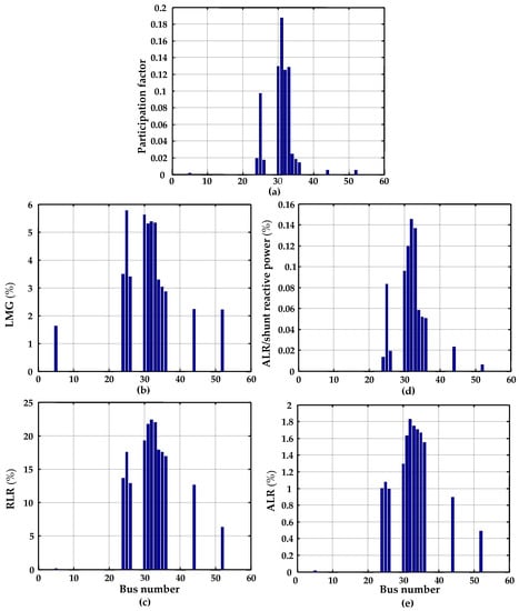
Figure 8.
Influence of 10 Mvar of shunt reactive power compensation at load bus of IEEE-57: (a) bus participation factors, (b) loading margin gain, (c) total reactive power losses reduction, (d) total active power losses reduction, normalized by shunt reactive power compensation (Table 5) and (e) total active power losses reduction.
Figure 9 shows the voltage profiles of the base case without and with the shunt reactive power compensation of 13.1128 MVar at bus 31, as obtained by the proposed method in Table 5. The improvement in the voltage profile of the base case followed by a reduction of about 2.2 MVar and 0.45 MW on the reactive and active power losses and an increase of about 7% in the loading margin can be verified, which represents an increase of about 22 MW (or 62 MVA) in the power transfer capacity. The respective generated reactive powers for the base case and after the shunt reactive power compensation are 326.4 MVar and 311.6 MVar. As a direct consequence, a reactive power reserve of 14.8 MVar is obtained in the generators, fulfilling with this the recommendations of the planning procedure related to reactive power compensation; to prevent or delay voltage collapse, one must create reactive reserves by bringing shunt capacitors into service as much as possible and/or reducing the transmission losses to allow existing generators to be run with an increased reactive margin [37].
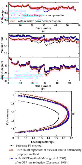
Figure 9.
Performance comparison of different methods for IEEE−57: (a) base case voltage profile improvement obtained by the inclusion of a capacitor bank at bus 31, and improvement on (b) voltage and angle profiles, and (c) P-V curves obtained with loss reduction procedures: inclusion of the shunt reactive power compensation by the proposed method, and from the converged state of MCPF and OPF methods [30,31].
Figure 9b shows the voltage and angle profiles obtained by the MCPF [30] and the OPF [31] methods, and considering the inclusion of capacitor banks obtained by the proposed method at buses 31 and 44, whose values are presented in the fifth column of Table 5. The voltage and angle profiles presented in Figure 9e show that the voltage profile of the base case is improved, while the angle profile is practically maintained. They also do not differ much from those obtained by the other two methods. The P-V curves traced by using a CPF are shown in Figure 9c. Their respective MLPs can be seen in the fourth column of Table 6, where a comparison between the performance of the methods is presented. By the inclusion of capacitor banks, the obtained loading margin is improved by about 21.3%, with a reactive power reserve (RPR) of 372.3 MVar in the generators (PV buses), i.e., an addition of 69.7 MVar in the base case value (302.6 MVar). A loading margin increase of 24.5% is provided, starting from both converged solutions of the OPF and MCPF methods. Nevertheless, at the expense of a respective reduction of 13.8 MVar and 96.5 MVar on the reserve of reactive power of the base case, it is needed for the base case real power losses reduction. Therefore, it can be concluded that the proposed method improves the loading margin and the voltage profile, comparable to the other two methods.
Table 6.
Comparison between the performances of the methods for the IEEE-57.
3.3. Performance of the Proposed Method to Determine the Total Reactive Power Loss Reduction (RLR) of IEEE-300
Figure 10a presents the P-V curves of the IEEE-300 system. This figure shows a system with voltage instability problems with strong local characteristics [38]. In this kind of system, a voltage profile of a small area, or voltage magnitude of only a few buses, does not remain within the normal range of operation. Moreover, the difference between the maximum loading point (λ = 1.0552 pu) and the base case (λ = 1), i.e., the loading margin, is approximately 5.52%, which shows that this is also a heavy-loaded system.
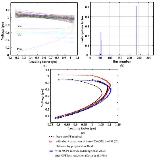
Figure 10.
IEEE-300 bus system with the reactive power limits of PV buses: (a) PV curves, (b) participating factor and (c) P-V obtained with loss reduction procedures: inclusion of the shunt reactive power compensation by the proposed method, and from the converged state of MCPF and OPF methods [30,31].
The five lowest eigenvalues and the results obtained by the method for the buses indicated by the first ten participation factors, corresponding to the lowest eigenvalue (2.817 × 10⁻⁷), are shown in Table 7 and Table 8, respectively. The first two columns of Table 8 indicate the bus numbers listed in the System Data and the respective internal numbers of the buses, in the order given by the participation factors (third column). Figure 10a and column 3 of Table 8 show the participation factor values. Columns 11 and 13 of Table 8 show the values of total reactive power losses reduction and loading margin increase per unit of the shunt capacitor bank. From these results, it can be concluded that the two main locations (buses) that are most efficient at performing shunt compensation in order to reduce the total reactive power losses and increase the loading margin are the buses 236 and 56. These are the same buses identified by participation factors of the critical mode as shown in Figure 10b. Note that buses 52–54 are also indicated by the proposed method as candidates for loading margin increase and total reactive power loss reduction.
Table 7.
Eigenvalues of IEEE-300 at MLP (λ = 1.0552 pu) considering the reactive power limits of PV buses.
Table 8.
Simulation results for the IEEE-300 obtained by the total reactive power losses versus bus voltage magnitude curve method considering the reactive power limits at PV buses (1.0552 pu, QlossBC = −247.5605 MVar; PlossBC = 421.5985).
Figure 11a–c present the values of participation factors, and of total reactive power losses reduction and loading margin increase per unit of the capacitor bank. Intending to compare the results provided by the analysis, Figure 11d,e present the respective percentages of loading margin increase (LMG) and total reactive power losses reductions (RLR) obtained with a shunt capacitor bank of 10 MVar applied separately at each one of the load buses indicated by the participation factor. Comparing these with the respective Figure 11b,c, the coherence of the results provided by the analysis can be confirmed.
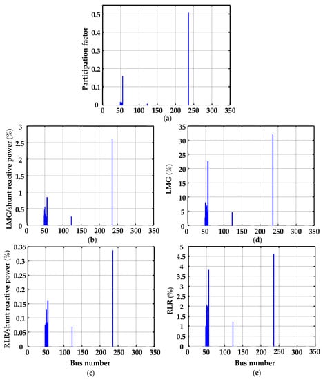
Figure 11.
Performance of the proposed method for IEEE-300: (a) bus participation factors, (b) loading margin increase, (c) total reactive power losses reduction, normalized by shunt reactive power compensation, and (d) loading margin increase and (e) total reactive power losses reduction, considering a shunt reactive power compensation of 10 MVar at each one of the load buses, as indicated by the participation factors of the critical mode.
Figure 10c shows the P-V curves traced by using a CPF starting from the converged solutions obtained by the MCPF and OPF methods [31], and considering the inclusion of capacitor banks obtained by the proposed method at buses 236 and 54, whose values are presented in the sixth column of Table 8. Their respective MLPs can be seen in the fourth column of Table 9, where a comparison between the performance of the methods is presented. By the inclusion of capacitor banks, the obtained loading margin is improved by about 131.2%, with a reactive power reserve (RPR) of 6831.4 MVar in the generators (PV buses), i.e., an addition of 795.3 MVar in the base case value (6036.3 MVar). Loading margin increases of 95.5% and 60.5% are provided starting from the respective converged state of the MCPF and OPF methods. The reserves of reactive power provided by the MCPF and OPF methods are 884.6 MVar and 407.3 MVar, respectively.
Table 9.
Comparison between the performances of the methods for the IEEE-300.
As can be seen from Table 8, as a consequence of the shunt reactive power compensation of 34.94 MVar only at bus 236, as indicated by the proposed method in Table 9, an improvement of about 91% in the loading margin was obtained, close to the 95% provided by the MCPF, and higher than that provided by the OPF. This improvement in the loading margin represents an increase of about 1181.00 MW (or 1244.03 MVA) in the power transfer capacity. Note that in this system, shunt capacitor banks of 55 and 325 MVAr can be found. The respective generated reactive powers for the base case and after the shunt reactive power compensation are 8131.26 MVar and 8066.94 MVAr. Furthermore, the compensation provides a reduction of about 29.11 MVar and 3.12 MW on the reactive and active power losses, respectively.
4. Conclusions
In this paper, an alternative methodology, based on the curve of the total reactive power losses versus the voltage magnitude of a chosen bus, is used to obtain the precise amount of shunt reactive power compensation in order to simultaneously reduce the total reactive power losses, improve the voltage profile and increase the loading margin. The participation factors obtained by applying static modal analysis indicate the best places for shunt reactive compensation. It was confirmed that the buses with more significant participation factors further increased the system load margin. Generally, they are also suitable for total reactive power loss reduction. From the proposed analysis, obtaining a significant load margin increase and loss reduction with shunt reactive power compensation was possible. Moreover, comparisons between the results obtained by the proposed method with those of an OPF and an MCPF procedure show that it can provide similar results for the loading margin increase. Thus, it can be a reasonable alternative to power system voltage stability enhancement.
Author Contributions
G.B.L.: conceptualization and original draft, A.B.N. and D.A.A.: conceptualization, writing—original draft, writing—review and editing, investigation and supervision. C.R.M.: conceptualization, writing—review and editing, and funding acquisition. E.d.S.A.: conceptualization and writing—review. L.C.P.d.S.: writing—review and editing. All authors have read and agreed to the published version of the manuscript.
Funding
This research received financial support provided by CNPq (Brazilian Research Funding Agencies) process 302896/2022-8, FAPESP process 2018/12353-9, and CAPES (Coordination for the Improvement of Higher Education Personnel)—Financing Code 001.
Data Availability Statement
No data are used in this article.
Acknowledgments
The authors are grateful for the financial support provided by CNPq (Brazilian Research Funding Agencies) process 302896/2022-8, FAPESP process 2018/12353-9, and CAPES (Coordination for the Improvement of Higher Education Personnel)—Financing Code 001.
Conflicts of Interest
The authors declare that they have no competing interests.
Nomenclature
| CPF | Continuation power flow |
| RPM | Reactive power margin |
| OPF | Optimal power flow |
| DG | Distributed generation |
| PSO | Particle swarm optimization |
| MCPF | Modified continuation power flow |
| pfki | Participation factor |
| Qloss | Total reactive power losses |
| LMG | Load margin increase |
| RPR | Reactive power reserve |
| RLR | Total reactive power losses reduction |
| MLP | Maximum loading point |
| ALR | Total active power losses reduction |
| P-V | Voltage versus active power curve |
| PV | Generation bus |
| PQ | Load bus |
| pu | Per unit |
| λ | Loading factor |
Appendix A
Procedure used to obtain the V−Qloss and Qgen−Qloss curves [1]. The curves are simultaneously produced by running a series of load flow cases.
- For a power flow base case, a fictitious synchronous condenser is added to a selected bus and the bus type is changed into a fictitious PV bus;
- Vary the condenser scheduled output voltage magnitude (V) in small steps (usually 0.01 pu or less);
- Solve the power flow case;
- Record the specified bus voltage magnitude (V) value, and by using (1) and (2), respectively, compute and store the corresponding values of total reactive power losses (Qloss—Equation (1)) and generated reactive power (Qgen—Equation (2));
- Repeat steps 2 to 4 until sufficient points have been collected;
- Plot the V−Qloss and Qgen−Qloss curves.
References
- Reactive Power Reserve Work Group, Voltage Stability Criteria, Undervoltage Load Shedding Strategy, and Reactive Power Reserve Monitoring Methodology. 1998, p. 154. Available online: http://www.wecc.biz/library/DocumentationCategorizationFiles/Guidelines (accessed on 13 April 2022).
- WECC-Western Electricity Coordinating Council, Final Report, Voltage Stability Criteria, Undervoltage Load Shedding Strategy, and Reactive Power Reserve Monitoring Methodology, Reactive Power Reserve Work Group, Salt Lake City. 1998. Available online: https://www.wecc.org/Reliability/Voltage%20Stability%20Criteria%20May%201998.pdf (accessed on 24 May 2022).
- Skliutas, J.P.; Aquila, J.M.F.; Konopinsk, R.; Marken, P.; Schartner, C.; Zhi, G. Planning the Future Grid with Synchronous Condensers. In Proceedings of the CIGRE US National Committee 2013 Grid of the Future Symposium, Paris, France, 6 July 2013; pp. 1–12. [Google Scholar]
- Masood, T.; Aggarwal, R.K.; Qureshi, S.A.; Khan, R.A.J. STATCOM model against SVC control model performance analyses technique by Matlab. In Proceedings of the International Conference on Renewable Energies and Power Quality, Granada, Spain, 23–25 March 2010. [Google Scholar]
- Igbinovia, F.O.; Fandi, G.; Müller, Z.; Švec, J.; Tlusty, J. Cost implication and reactive power generating potential of the synchronous condenser. In Proceedings of the 2nd International Conference on Intelligent Green Building and Smart Grid, Prague, Czech Republic, 27–29 June 2016; pp. 1–6. [Google Scholar]
- Oliveira, C.C.; Bonini Neto, A.; Alves, D.A.; Minussi, C.R.; Castro, C.A. Alternative Current Injection Newton and Fast Decoupled Power Flow. Energies 2023, 16, 2548. [Google Scholar] [CrossRef]
- Karimi, M.; Shahriari, A.; Aghamohammadi, M.R.; Marzooghi, H.; Terzija, V. Application of Newton-based load flow methods for determining steady state condition of well and ill-conditioned power systems: A review. Electr. Power Energy Syst. 2019, 113, 298–309. [Google Scholar] [CrossRef]
- Bonini Neto, A.; Magalhães, E.M.; Alves, D.A. Geometric Parameterization Technique for Continuation Power Flow Based on Quadratic Curve. Electr. Power Compon. Syst. 2018, 45, 1–13. [Google Scholar] [CrossRef]
- Portelinha, R.K.; Durce, C.C.; Tortelli, O.L.; Lourenço, E.M. Fast-decoupled power flow method for integrated analysis of transmission and distribution systems. Electr. Power Syst. Res. 2021, 196, 107215. [Google Scholar] [CrossRef]
- Bonini Neto, A.; Alves, D.A.; Minussi, C.R. Artificial Neural Networks: Multilayer Perceptron and Radial Basis to Obtain Post-Contingency Loading Margin in Electrical Power Systems. Energies 2022, 15, 7939. [Google Scholar] [CrossRef]
- Matarucco, R.R.; Bonini Neto, A.; Alves, D.A. Assessment of branch outage contingencies using the continuation method. Electr. Power Energy Syst. 2014, 55, 74–81. [Google Scholar] [CrossRef]
- Souza, A.C.Z.; Mohna, F.W.; Borges, I.F.; Ocariz, T.R. Using PV and QV curves with the meaning of static contingency screening and planning. Electr. Power Syst. Res. 2011, 81, 1491–1498. [Google Scholar] [CrossRef]
- Mousavi, O.M.; Cheekaoui, R. Investigation of P-V and V-Q based optimization methods for voltage and reactive power analysis. Int. J. Electr. Power Energy Syst. 2014, 63, 769–778. [Google Scholar] [CrossRef]
- Gao, B.; Morison, G.K.; Kundur, P. Voltage stability evaluation using modal analysis. IEEE Trans. Power Syst. 1992, 7, 1529–1542. [Google Scholar] [CrossRef]
- Feng, Z.; Xu, W.; Oakley, C.; McGoldrick, S. Experiences on assessing Alberta power system voltage stability with respect to the WSCC reactive power criteria. In Proceedings of the Power and Energy Society Summer Meeting, Edmonton, AB, Canada, 18–22 July 1999; pp. 1297–1302. [Google Scholar]
- Sharif, S.S.; Taylor, J.H.; Hill, E.F.; Scott, B.; Daley, D. Real–time implementation of optimal reactive power flow. IEEE Power Eng. Rev. 2000, 20, 47–51. [Google Scholar] [CrossRef]
- Dong, F.; Chowdhury, B.H.; Acar, L.; Crow, M. Cause and effects of voltage collapse-case studies with dynamic simulations” (2005). In Proceedings of the Power Engineering Society General Meeting, Denver, CO, USA, 6–10 June 2004; Volume 2, pp. 1806–1812. [Google Scholar]
- Menezes, T.V.; Silva, L.C.P.; Affonso, C.M.; Costa, V.F. MVAR management on the pre-dispatch problem for improving voltage stability margin. IET Gener. Transmiss. Distrib. 2004, 151, 665–672. [Google Scholar] [CrossRef]
- Affonso, C.M.; Silva, L.C.P.; Lima, F.G.M. MW and MVar Management on supply and demand side for meeting voltage stability margin criteria. IEEE Trans. Power Syst. 2004, 19, 1538–1545. [Google Scholar] [CrossRef]
- Raoufi, H.; Kalantar, M. Reactive power rescheduling with generator ranking for voltage stability improvement. Energy Convers. Manag. 2009, 50, 1129–1135. [Google Scholar] [CrossRef]
- Omidi, H.; Mozafari, B.; Parastar, A.; Khaburi, M.A. Voltage stability margin improvement using shunt capacitors and active and reactive power management. In Proceedings of the IEEE Electrical Power & Energy Conference, Montreal, QC, Canada, 22–23 October 2009; pp. 1–5. [Google Scholar]
- Feng, D.; Chowdhury, B.H.; Crow, M.L.; Acar, L. Improving voltage stability by reactive power reserve management. IEEE Trans. Power Syst. 2005, 20, 338–345. [Google Scholar] [CrossRef]
- Ntombela, M.; Musasa, K.; Leoaneka, M.C. Power Loss Minimization and Voltage Profile Improvement by System Reconfiguration, DG Sizing, and Placement. Computation 2022, 10, 180. [Google Scholar] [CrossRef]
- Tripathy, M.; Mishra, S. Bacteria foraging-based solution to optimize both real power loss and voltage stability limit. IEEE Trans. Power Syst. 2007, 22, 240–248. [Google Scholar] [CrossRef]
- Amgad, A.E.D.; Youssef, K.M.H.; EL-Metwally, M.M.; Osman, Z. Optimum VAR sizing and allocation using particle swarm optimization. Electr. Power Syst. Res. 2007, 77, 965–972. [Google Scholar] [CrossRef]
- Aman, M.M.; Jasmon, G.B.; Bakar, A.H.A.; Mokhlis, H. A new approach for optimum DG placement and sizing based on voltage stability maximization and minimization of power losses. Energy Convers. Manag. 2013, 70, 202–210. [Google Scholar] [CrossRef]
- Sirjani, R.; Mohamed, A.; Shareef, H. Optimal allocation of shunt Var compensators in power systems using a novel global harmony search algorithm. Int. J. Electr. Power Energy Syst. 2012, 43, 562–572. [Google Scholar] [CrossRef]
- Yang, C.F.; Lai, G.G.; Lee, C.H.; Su, C.T.; Chang, G.W. Optimal setting of reactive compensation devices with an improved voltage stability index for voltage stability enhancement. Int. J. Electr. Power Energy Syst. 2012, 37, 50–57. [Google Scholar] [CrossRef]
- Poornazaryan, B.; Karimyan, P.; Gharehpetian, G.B.; Abedi, M. Optimal allocation and sizing of DG units considering voltage stability, losses and load variations. Int. J. Electr. Power Energy Syst. 2016, 79, 42–52. [Google Scholar] [CrossRef]
- Malange, F.C.V.; Alves, D.A.; Silva, L.C.P.; Castro, C.A.; Costa, G.R.M. Real power losses reduction and loading margin improvement via continuation method. IEEE Trans. Power Syst. 2003, 19, 1690–1692. [Google Scholar] [CrossRef]
- Costa, G.R.M.; Langona, K.; Alves, D.A. A new approach to the solution of the optimal power flow problem based on the modified Newton’s method associated to an augmented Lagrangian function. In Proceedings of the IEEE International Conference on Power System Technology, Beijing, China, 18–21 August 1998; pp. 909–913. [Google Scholar]
- Monticelli, A.J. Load Flow in Electric Power Networks; Edgard Blucher: São Paulo, Brazil, 1983. [Google Scholar]
- Alves, D.A.; Silva, L.C.P.; Castro, C.A.; Costa, V.F. Study of alternative schemes for the parameterization step of the continuation power flow method based on physical parameters, part I: Mathematical modelling. Electr. Power Compon. Syst. 2003, 31, 1151–1166. [Google Scholar] [CrossRef]
- Alves, D.A.; Silva, L.C.P.; Castro, C.A.; Costa, V.F. Study of alternative schemes for the parameterization step of the continuation power flow method based on physical parameters, part II: Performance Evaluation. Electr. Power Compon. Syst. 2003, 31, 1167–1177. [Google Scholar] [CrossRef]
- Ajjarapu, V.; Christy, C. The continuation power flow: A tool for steady state voltage stability analysis. IEEE Trans. Power Syst. 1992, 7, 416–423. [Google Scholar] [CrossRef]
- Souza, A.C.Z.; Cañizares, C.A.; Quintana, V.H. New techniques to speed up voltage collapse computations using tangent vectors. IEEE Trans. Power Syst. 1997, 12, 1380–1387. [Google Scholar] [CrossRef]
- Cigre Working Group 38-01, Task Force No 03, Brochure 30, Reactive power compensation analyses and planning procedure, CIGRE Paris. 1989. Available online: https://e-cigre.org/publication/030-reactive-power-compensation-analyses-and-planning-procedure (accessed on 14 June 2023).
- Bonini Neto, A.; Alves, D.A. Improved geometric parameterization techniques for continuation power flow. IET Gener. Transmiss. Distrib. 2010, 4, 1349–1359. [Google Scholar] [CrossRef]
Disclaimer/Publisher’s Note: The statements, opinions and data contained in all publications are solely those of the individual author(s) and contributor(s) and not of MDPI and/or the editor(s). MDPI and/or the editor(s) disclaim responsibility for any injury to people or property resulting from any ideas, methods, instructions or products referred to in the content. |
© 2023 by the authors. Licensee MDPI, Basel, Switzerland. This article is an open access article distributed under the terms and conditions of the Creative Commons Attribution (CC BY) license (https://creativecommons.org/licenses/by/4.0/).