Integrating Demand Response for Enhanced Load Frequency Control in Micro-Grids with Heating, Ventilation and Air-Conditioning Systems

Abstract

Heating, ventilation and air-conditioning (HVAC) systems constitute the majority of the demands in modern power systems for aggregated buildings. However, HVAC integrated with renewable energy sources (RES) face notable issues, such as uneven demand–supply balance, frequency oscillation and significant drop in system inertia owing to sudden disturbances in nearby generation for a longer period. To overcome these challenges, load frequency control (LFC) is implemented to regulate the frequency, maintain zero steady-state error between the generation and demand, reduce frequency deviations and balance the active power flow with neighboring control areas at a specified value. In view of this, the present paper investigates LFC with a proposed centralized single control strategy for a micro-grid (µG) system consisting of RESs and critical load of a HVAC system. The proposed control strategy includes a newly developed cascaded two-degree-of-freedom (2-DOF) proportional integral (PI) and proportional derivative filter (PDF) controller optimized with a very recent meta-heuristic algorithm—a modified crow search algorithm (mCSA)—after experimenting with the number of performance indices (PICs). The superiority of both the proposed optimization algorithm and the proposed controller is arrived at after comparison with similar other algorithms and similar controllers, respectively. Compared to conventional control schemes, the proposed scheme significantly reduces the frequency deviations, improving by 27.22% from the initial value and reducing the performance index criteria (ƞ_ISE) control error to 0.000057. Furthermore, the demand response (DR) is implemented by an energy storage device (ESD), which validates the suitability of the proposed control strategy for the µG system and helps overcome the challenges associated with variable RESs inputs and load demand. Additionally, the improved robustness of the proposed controller for this application is demonstrated through sensitivity analysis with ±20% μG coefficient variation.

1. Introduction

The combustion of coal in thermal power plants to generate electricity contributes to an increase in the global carbon footprint, which, in turn, has a detrimental impact on the climate and the environment. In recent years, countries worldwide have collaborated to invest in renewable energy sources (RES) in order to mitigate the negative impacts of this growing carbon footprint. Popular RES options include photovoltaic (PV) systems, wind turbine generation systems (WTS), heat pump generating systems (HPG), bio-diesel generation systems (BDG) and fuel cells (FC). These RESs can be utilized in micro-grids (µG), which help meet the increasing demand for power [1] in a greener way. In some cases, micro-grids supply power to critical loads, such as freezers, heating, ventilation and air-conditioning (HVAC) systems, which have experienced a sudden surge in demand worldwide, as depicted in Figure 1 [2,3,4,5,6]. This highlights the impact of rising demand on the power industry. Moreover, the unpredictability, volatility and intermittency of RESs, along with the fluctuating demands of these critical loads, pose significant challenges for micro-grids, similar to those faced by conventional grid systems. These challenges make it very difficult to regulate the power output of micro-grids, resulting in rapid frequency deviations, which hinder power exchange between control areas with higher control errors. Unlike traditional grids, researchers working on micro-grid systems are focused on developing suitable control techniques, particularly load frequency control (LFC), to mitigate frequency oscillations and power-sharing issues [7].

LFC encompasses two techniques: (i) intelligent controller design and (ii) demand response (DR) management [8]. Recent research has explored various methods utilizing both of these LFC techniques, demonstrating notable mitigating impacts in micro-grid challenges. Therefore, LFC is a crucial approach aimed at maintaining the nominal system frequency by minimizing frequency variations caused by rapid changes in load and/or fluctuations in power output of RES [9].

Extensive research has been conducted on the first LFC technique, which involves designing an intelligent controller for the µG system. Several notable recent papers on this topic can be found in the literature [10,11,12,13]. Additionally, various controllers, such as the conventional PI controller [14], fractional order fuzzy-based PID (FOFPID) controller [15], fractional order proportional plus integral (FOPI) controller [16], cascaded controller of 1 + PI and C-PDF [17], multi-stage PID (MS-PID) structure with (P+DF) followed by a filter and a second stage of (1 + PI) [18], multi-stage PDF+ (1 + PI) controller [19] and fuzzy cascaded PD-PI controller [20], have demonstrated satisfactory performance in frequency response for both single-area and multi-area µG systems. However, the tuning of these controllers plays a crucial role in improving their performance. Therefore, various techniques have been employed in the literature to tune the controller parameters for LFC in the µG.

Various classical methods can be employed to regulate the parameters of the controller for LFC, including Ziegler–Nichols ultimate-cycle tuning, Cohen–Coon and Astrom– Hagglund [21]. However, the conventional optimization approach is not preferred when dealing with a large number of parameters. Consequently, there is a growing interest in utilizing soft computing approaches to fine-tune the control variables [22]. In the current state of the art, several meta-heuristic approaches [23] have been applied to estimate the optimal control parameters for LFC in µG. Examples of such approaches include the genetic algorithm (GA) proposed by Ref [14], the mind blast algorithm (MBA) introduced by Ref [24], an improved mouth swarm algorithm (IMSA) [25], a more efficient grasshopper optimization algorithm (GOA) [19], a green leaf-hopper flame optimization algorithm (GLFOA) [26], cohort intelligent optimization [27] and double deep Q-learning algorithm [28], among others. However, in order to find a feasible solution and improve dynamic responses, it is crucial to explore modern meta-heuristic algorithms, which offer enhanced explorative and exploitative search capabilities. Therefore, in this paper, the newly explored algorithm shows satisfactory results when combined with a suitable proposed controller.

In addition to the first technique of LFC, another state-of-the-art method is the DR, which offers a potential solution to power system issues through low inertia devices [29]. DR management involves the use of various energy storage devices (ESDs), as discussed in previous research, such as battery energy storage systems (BES) [30], saturable reactors (SR) [31], electric vehicles (EV) [32], super capacitor energy storage (SCEC) [33] and others. This technique demonstrates a significant reduction in frequency deviations during sudden disturbances. Another approach of DR in LFC is utilized by controlling the critical loads at the consumer side, which decreases the total network losses by 2.5% and reduces frequency deviation [34]. In this case, DR management operates with a localized controller by using thermostatic devices through the ON/OFF switching method. Furthermore, Ref [35] studied the concept of DR using a heating and ventilation cooperative home energy management system (CHoEMS), where critical loads, such as a HVAC system, play an important role in LFC because it has been observed that HVAC consumes more power than other loads, as discussed earlier in this paper. Additionally, recent local control schemes for LFC include under-frequency load shedding control scheme [36], a switching-based event-triggered control approach to demand side management [37], primary frequency regulation (PFR) and secondary frequency regulation (SFR) [38], and HVAC control [39], etc. However, a drawback of these localized control approaches is their proper coordination with the central controller, which may cause customer discomfort due to sudden curtailment of a large number of loads [40]. Therefore, a centralized control scheme is more suitable for controlling generators and demands, with a separate DR control utilizing ESDs [41]. Few investigations have explored different coordinated control strategies using the µG model, incorporating critical loads, such as freezers, heat pumps and plug-in electric vehicles (PHEV) [41,42]. Nevertheless, to evaluate the reduction in frequency deviations using a centralized single control scheme in the µG, various RESs and HVAC systems can be considered, particularly for the step changes in demand, which is the primary focus of this paper, as shown in Figure 2.

Based on the aforementioned literature, the significance of a centralized control strategy in a µG comprising various RESs, ESDs and HVAC systems was designed and simulated for validation. Therefore, this paper proposes an intelligent cascaded control scheme aimed at minimizing frequency deviations and maintaining a balance between generation and demand. Further, the parameters of the controller are optimized with a very recent meta-heuristic algorithm for the first time. The adoption of a cascaded controller in this study enhances the control capabilities within the newly developed µG (as depicted in Figure 2). This approach addresses the potential limitations of individual controllers, which may struggle to perform optimally and lead to reduced peak deviations. However, it should be noted that the secondary control loop of the cascaded controller has the drawback of slightly slower operations. Nevertheless, it significantly reduces peaks compared to a single primary control loop of the cascaded controller, as discussed later in the Results and Analysis section.

The main contributions in this paper are listed below:

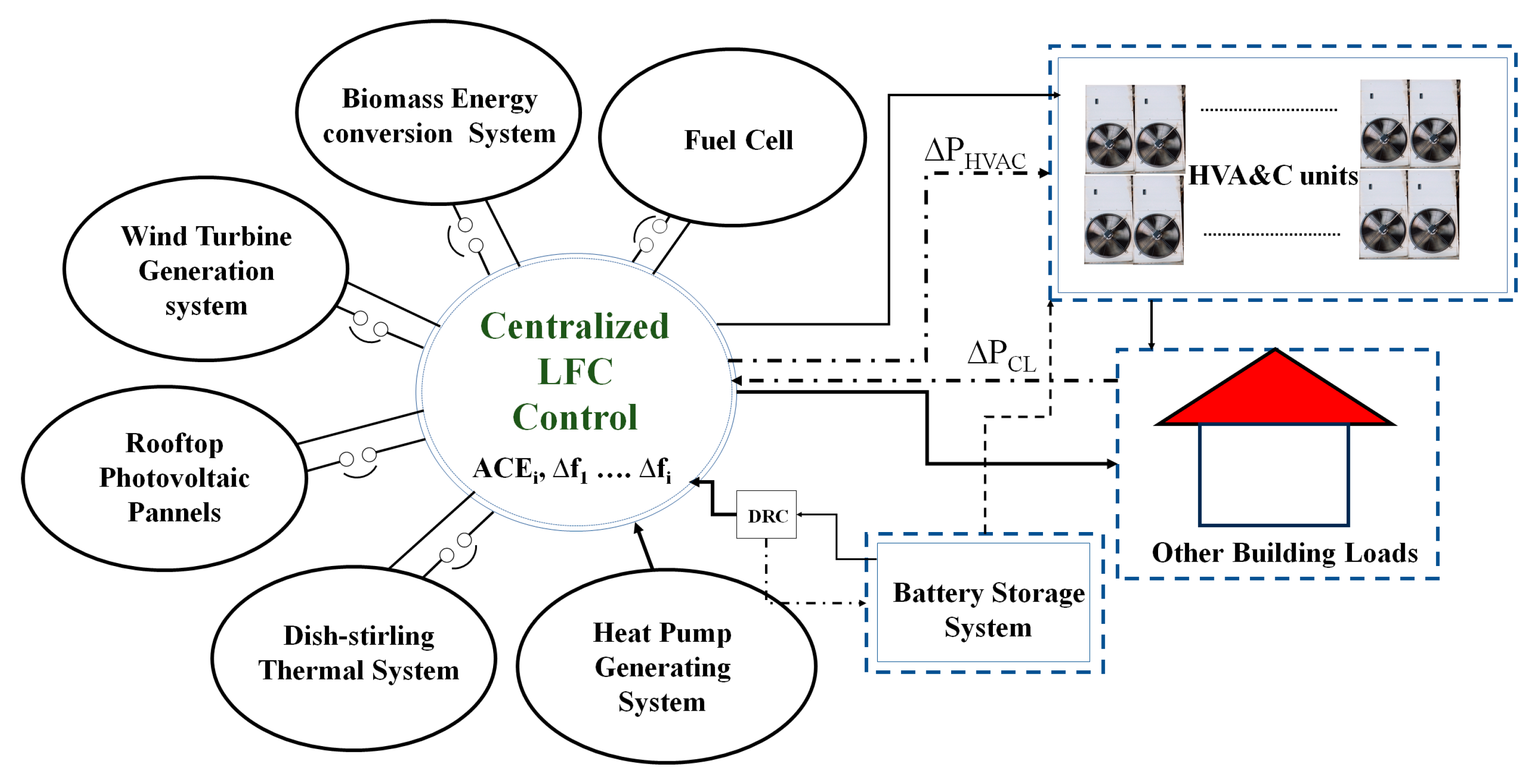
• Development of a micro-grid (µG) model for simulation in MATLAB/Simulink, including an integrated HPG system, RESs (PV, DSTS, WTS, FC), an ESD unit and a developed HVAC system as a critical load. This integration is a novel approach.
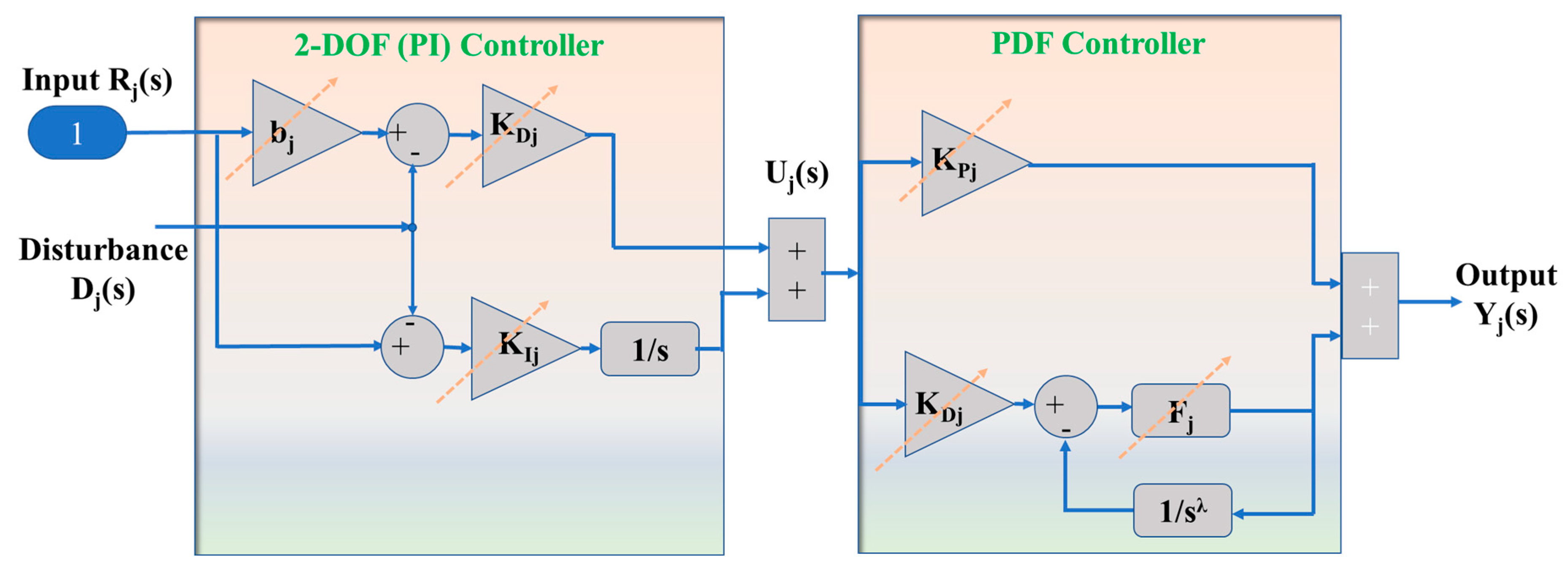
• A new cascaded 2-DOF (PI) and PDF controller is proposed and optimized with a number of recent meta-heuristic search algorithms, including the modified crow search algorithm (mCSA) considering the number of performance indices (PICs) for comparison before finalization regarding the best optimization algorithm and best PIC for reducing the frequency deviation in the µG system.
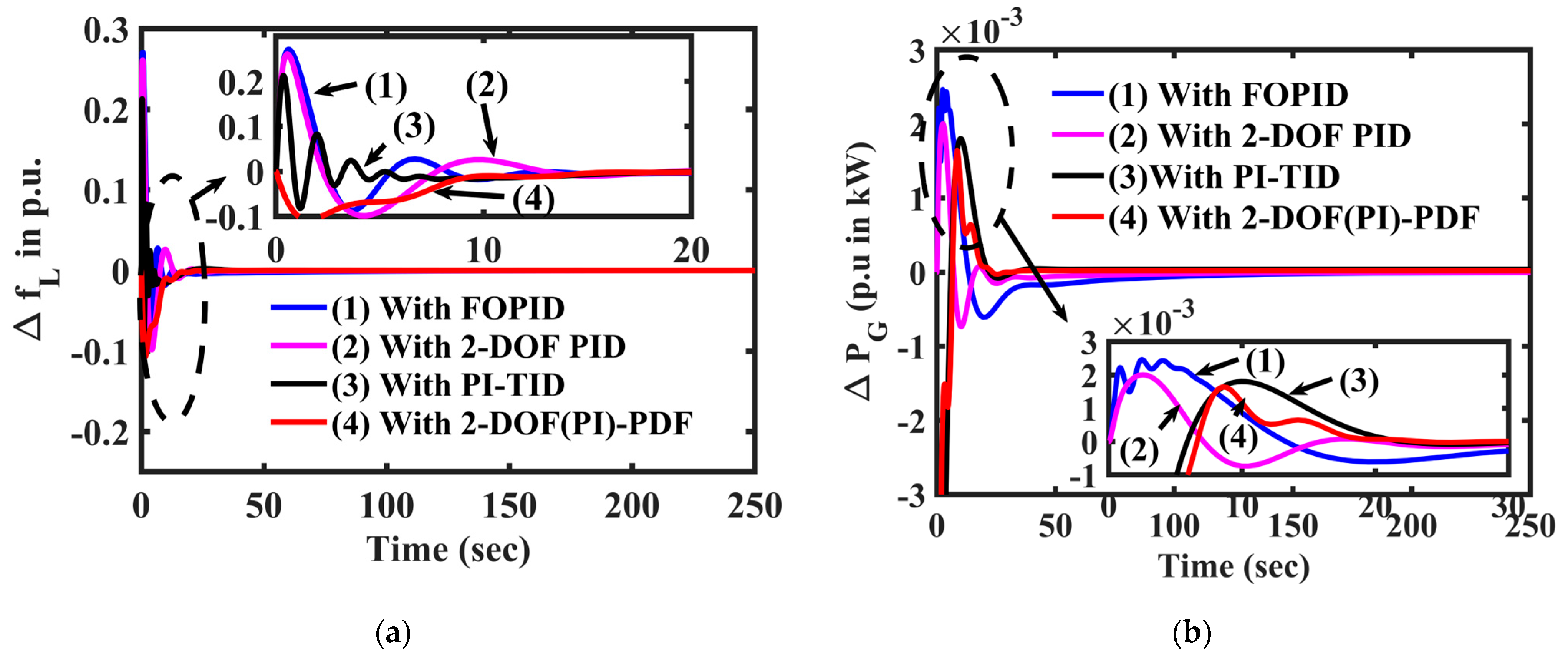
• The superiority of the proposed new cascaded controller as above is established after comparing its dynamic performance with other similar controllers, such as FOPID, 2-DOF with PID and PI-TID, in terms of the settling time, peak overshoot and undershoot and number of oscillations.
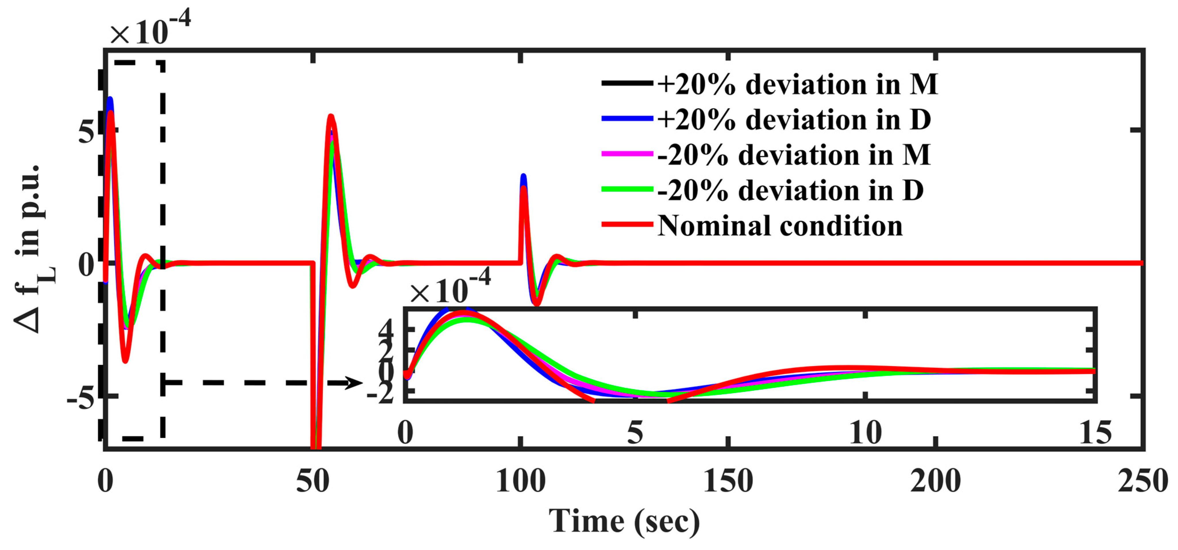
• To enhance the dynamic behavior using the proposed control scheme, DR management and a sensitivity analysis of different loading conditions are conducted for different scenarios.

The article is structured as follows. Section 2 illustrates the proposed model and the problem statement. The system components introduced in Section 2 are discussed in Section 3 in detail. The theoretical approach for the proposed control strategy with various recent optimization techniques for this proposed µG model is addressed in Section 4. The theoretical background and control strategy discussed in the previous sections are investigated further, and the simulation results with a conclusion are presented in Section 5 and Section 6, respectively.

2. Investigation of HVAC Integrated µG System

The detailed mathematical modeling of the proposed µG model is discussed in this Section and is shown in Figure 3a. The energy generation unit of the proposed µG is HPG, as the main governing generation system with capacity of 400 kW. Additionally, several other renewable energy generation units, including PV, WT, FC and DSTS, are integrated, with 100 kW generation capacity for each unit. To ensure flexibility in managing the demand and surplus energy, the BES system, functioning as the ESD, with a capacity of 250 kW, is considered. Consequently, the total power generation capacity of the µG amounts to 1000 kW. In addition to the power generation units, the system incorporates temperature-sensitive loads associated with the HVAC system. These loads are regulated by a central controller to accommodate any disturbances resulting from step load changes (∆P_CL). The output power of the proposed µG is expressed in Equation (1).

$$P_g=P_{HPG}+P_{PV}+P_{WTG}+P_{DSTS}+P_{FC}\pm P_{ESD}$$

(1)

where the solar insolation (∆ϕ) input to be considered for the simulation is 0.1 p.u.; the input variation of the WTS (∆ν) is considered to be 0.1 p.u.; and the output power from the fuel cell generation unit is considered to be 0.1 p.u. The other system parameter values, which are considered for designing the transfer function model of µG, are given in

Table 1. Model constraints and their values.

Parameter	Values (p.u.)
KPV, τPV [14]	1, 1.8
KWTS, τWTS [14]	1, 1.5
KDSTS, τDSTS [43]	1, 0.5
KFC, τFC [44]	1, 0.1
kGen, τGen,1, τGen,2, τgov, τTur [11]	0.25, 0.1, 0.2, 0.1, 0.3
KESD, τESD [45]	−0.003, 1
State of charge (SOC) [45]	With ideal conditions
KTH, TTH [46]	5, 5.5
KTcom, TTcom [47]	1, 3
a0, a1, a2, b0, b1 and b2 [48]	0.37, 0.01, 0.43, 0.00108, 0.017, 1
KE, TE [49]	1, 0.8
J, B [49]	1, 0.3
M, D [45]	0.2, 0.3

.

All RESs are expected to supply maximum power using power electronics converters/networks. Let the sudden variation in power from RESs cause deviations in output power to the load and other sensitive critical loads of the HVAC system (∆P_HVAC). To lessen the discrepancy (∆P_G) between the load and the generation, the suggested 2-DOF (PI) and PDF controller is used to regulate the frequency change (∆f_L) of the µG system.

$$\mathsf{\Delta }{P}_G=\mathsf{\Delta }{P}_g-\mathsf{\Delta }{P}_{CL}-\mathsf{\Delta }{P}_{HVAS}$$

(2)

The overall transfer function for the proposed µG is considered as

$$G_{sys}(s)=\frac{\mathsf{\Delta }{f}_L}{\mathsf{\Delta }{P}_G}=\frac{1}{Ms+D}$$

(3)

Problem Formulation of Proposed µG

The proposed µG in Equation (3) is investigated with the suitable control strategy. In the proposed control scheme, the recent algorithm is used to tune the newly approached suggested 2-DOF (PI) and PDF [34] controller parameters in order to minimize the PIC (ƞ) [50].

$$\begin{array}{l}{\mathsf{\eta }}_{\mathrm{ISE}}={\displaystyle \underset{0}{\overset{t}{\int }}{|\mathsf{\Delta }\mathrm{f}}_L{|}^2\mathrm{dt}}\\ {\mathsf{\eta }}_{\mathrm{ITSE}}={\displaystyle \underset{0}{\overset{t}{\int }}{|\mathsf{\Delta }\mathrm{f}}_L{|}^2\times \mathrm{tdt}}\\ {\mathsf{\eta }}_{\mathrm{IAE}}={\displaystyle \underset{0}{\overset{t}{\int }}{|\mathsf{\Delta }\mathrm{f}}_L|\mathrm{dt}}\\ {\mathsf{\eta }}_{\mathrm{ITAE}}={\displaystyle \underset{0}{\overset{t}{\int }}{|\mathsf{\Delta }\mathrm{f}}_L|\times t\mathrm{dt}}\end{array}\}$$

(4)

The equation mentioned above is derived to assess the effectiveness of the proposed control scheme, as illustrated in Figure 3b and discussed in Section 4. This control scheme is developed after designing each component of the micro-grid, as explained in Section 3.

3. System Components and Their Description

In this section, the abovementioned system components with various RES units are concisely described in Section 3.1, Section 3.2, Section 3.3, Section 3.4, Section 3.5 and Section 3.6. The integrated HVAC system for modern µG is also described briefly in Section 3.7.

3.1. Proposed Heat Pump Generating System Modeling

In this article, the heat pump generating unit is the dispatchable unit for droop control. The working principle of the HPG replicates the thermal generation units described in Ref [51]. Therefore, it has three main components working simultaneously, namely the governor, turbine and the generator, where the governor has two inputs of ∆P_r and ∆ω_v. Small perturbations can cause changes in the governor output [11]:

$$\mathsf{\Delta }{P}_{gov}=\mathsf{\Delta }{P}_r-\frac{1}{R}\mathsf{\Delta }{\omega }_v\text{kW}$$

(5)

The variation in the valve position of ∆x_v causes a change in the output of ∆P_v and ∆P_gov. Hence

$$\mathsf{\Delta }{x}_v=\mathsf{\Delta }{P}_{gov}-\mathsf{\Delta }{P}_v\text{kW}$$

(6)

where

$$\mathsf{\Delta }{P}_v=k_y{\displaystyle \int \mathsf{\Delta }{x}_v}dt$$

(7)

Therefore, the transfer function for the governor of the plant is

$$G_{gov}=\frac{\mathsf{\Delta }{P}_v}{\mathsf{\Delta }{P}_{gov}}=\frac{1}{1+{\tau }_{gov}}$$

(8)

For the turbine, it is assumed that the output mass flow is proportional to the pressure of the vessel at constant temperature. Therefore, the turbine leads to a first-order transfer function, and the generator maintains unaltered constant output. Therefore, the transfer function equations of the turbine and HPG are given by

$$\mathsf{\Delta }{P}_{Tur}=\frac{1}{1+s{\tau }_{Tur}}\mathsf{\Delta }{P}_{gov}$$

(9)

$$G_{HPG}=\frac{\mathsf{\Delta }{P}_v}{\mathsf{\Delta }{P}_{HPG}}=\frac{k_G\left(1+s{\tau }_{Gen,2}\right)}{\left(1+s{\tau }_{gov}\right)\left(1+s{\tau }_{Tur}\right)\left(1+s{\tau }_{Gen,1}\right)}$$

(10)

The notation is given in the nomenclature. Thus, the HPG power deviation equation of ∆P_HPG associated with Equation (1) for the LFC study is shown in Figure 3a, and the value of the parameter is given in Table 1.

3.2. Solar PV System

A new era of solar integrated building PV systems is part of the recent developments in renewable energy harvesting. Further, the cost-effective PV system components facilitate the PV technology to be the prime renewable energy source for future electrical demands. However, the building generation system with PV makes it even more robust, and its transfer function for LFC analysis is given in Equation (11) [14]:

$$G_{PV}=\frac{K_{PV}}{1+s{\tau }_{PV}}$$

(11)

3.3. Wind Turbine System (WTS)

Wind power is a commonly used renewable energy source (RES), which offers advantages in reducing carbon emissions compared to fossil fuels. In this micro-grid (µG) system, a horizontal wind turbine is connected to high-efficiency power electronic converters to optimize energy generation. For the purposes of this article, it is assumed that the output of the WTS is fixed at 0.1 p.u. in order to evaluate the performance of the proposed µG system controller. The transfer function model of the WTS for LFC is represented by [52]

$$G_{WTG}=\left(\frac{K_{WTG}}{1+s{\tau }_{WTG}}\right)$$

(12)

3.4. Dish–Stirling Solar System (DSTS)

Approximately 2–50 MW can be produced for µG and small-scale applications. A lack of PV capacity to satisfy peak demand may result from diurnal temperature fluctuations. As a result, the DSTS stores heat and turns it into usable power. A first-order transfer function model in Equation (13) is taken into account for the proposed μG [43], while the usage is further discussed in Section 5.4.

$$G_{DSSP}=\frac{K_{DSTS}}{1+s{\tau }_{DSTS}}$$

(13)

3.5. Fuel Cell

The electrochemical reaction of hydrogen and oxygen in a fuel cell produces energy. Unlike typical generators, such as diesel generators, fuel cells can produce power without making noise or polluting the environment. They generate a low dc voltage, which can be converted to AC using more efficient power converters. Therefore, a large-scale FC can be implemented in the µG era. A first-order lag transfer function model is used for this LFC analysis [44], given in Equation (14):

$$G_{FC}=\frac{K_{FC}}{1+s{\tau }_{FC}}$$

(14)

3.6. Energy Storage Device

For the study, a Li-polymer battery storage device is considered for area-1, and its transfer function equation in Ref. [45] is given by

$$G_{ESD}=\frac{K_{ESD}}{\left(1+s{\tau }_{ESD}\right)}$$

(15)

The controlled DR unit has to be defined in such a way, so as to neglect the minimum variation in ∆f_L by controlling the output of the ESD unit. In this model, the variation can be measured by Equation (16) [34]:

$$P_{DRC}=\left(\frac{△f_L}{△f}\right)\left(△P_G+k_t△T\right)$$

(16)

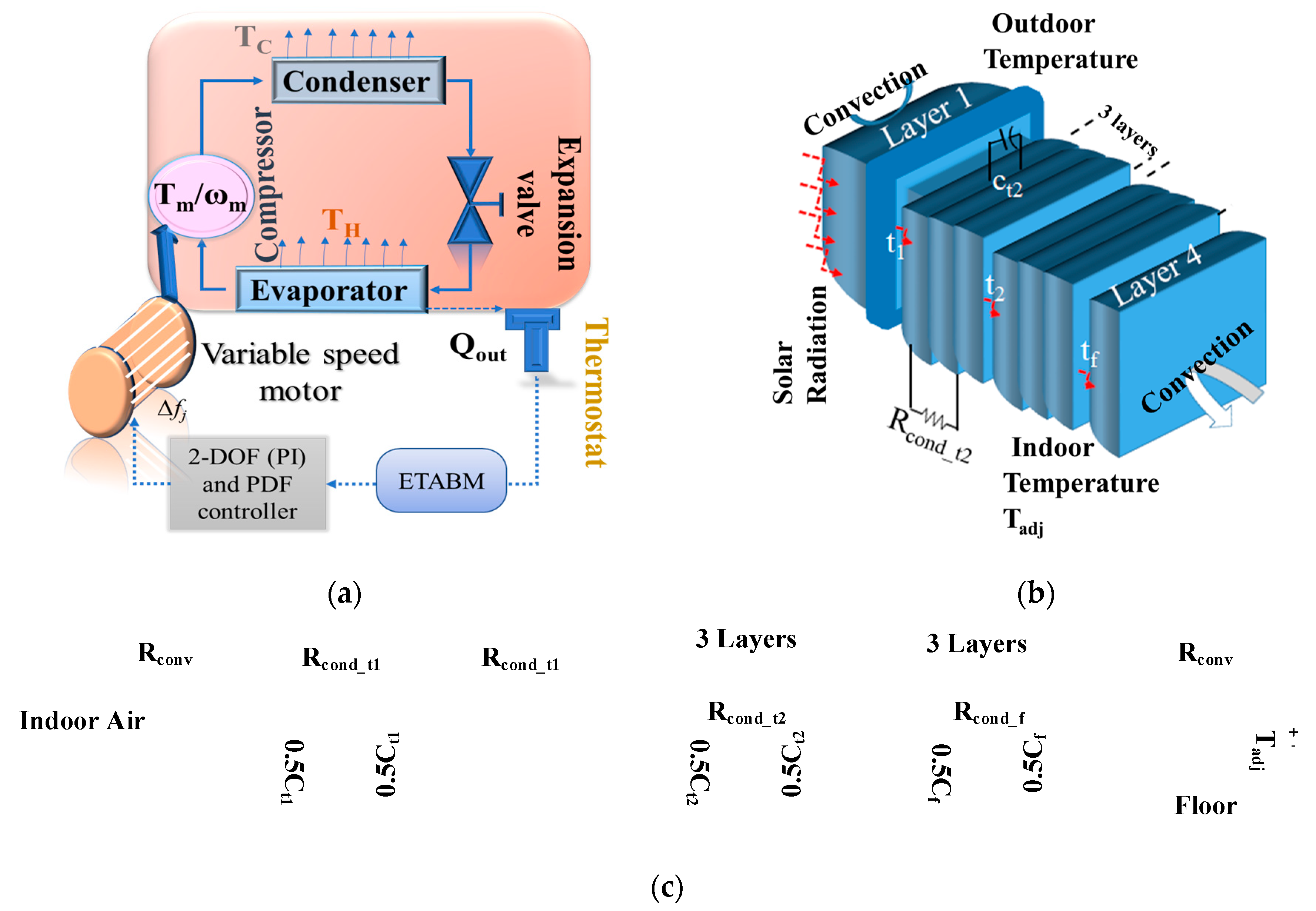
3.7. Proposed Heating, Ventilation and Air-Conditioning System (HVAC) for Aggregated Building Model

The proposed micro-grid (µG) incorporates a HVAC system consisting of a variable speed heat pump (VSHP), an equivalent thermal activated building model (ETABM) and a thermostat device. Figure 4a illustrates the comprehensive structure of the HVAC system, and the subsequent sections will delve into the details of each component.

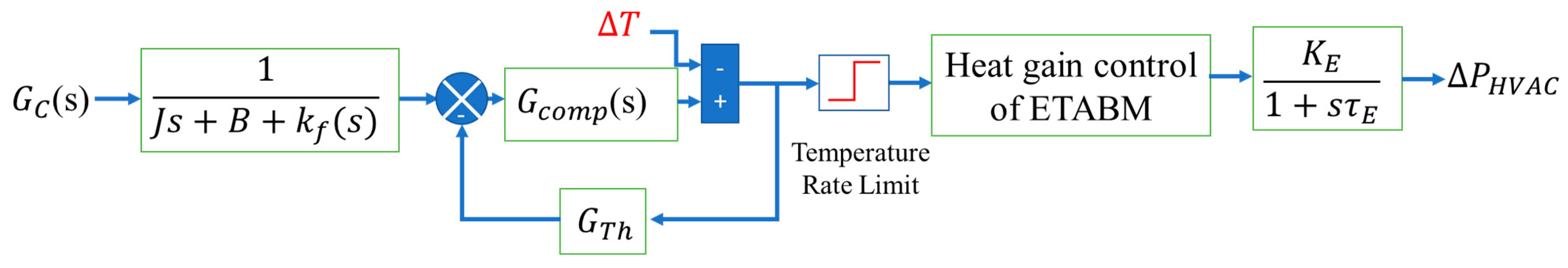
3.7.1. Variable Speed Heat Pump (VSHP) for HVAC

The working principle of a VSHP is similar to a Rankin cycle. A VSHP is the heat pump coupled to a variable speed induction motor [53]; its function is to control the room temperature by controlling the HVAC inputs. The complete aggregated model of the VSHP for the proposed µG system is shown in Figure 4a. In this model, the components of the VSHP are the compressor, the condenser (converting gas to a liquid condition), the expansion valve and the evaporator (converting liquid to a gaseous state). The main component of the VSHP is the compressor. This compressor speed adjusts the indoor temperature by controlling the fuel injection rate. Therefore, the compressor’s mechanical output or shaft speeds are linearly dependent on the temperature [54], which results in frequency regulations. It is assumed that the fan power consumption is neglected for the proposed aggregated model; then, the output mechanical power is expressed as in Equation (17) with different speeds (ω_r) and temperatures [49]:

$$P_{ms}=k_w{\omega }_r+k_c{T}_{ec}+k_e{T}_{eH}+k_{offset}$$

(17)

The coefficients of k_w, k_c, k_e, k_offset, T_ec and T_eh are determined by the number of regressive polynomial algorithms, lower and upper limit temperature. The output mechanical power fluctuations of the VSHP ∆P_m during instability are expressed as [49]

$$\mathsf{\Delta }{P}_m(s)=\frac{n^{\varphi }{}_{\omega 1}s+n^{\varphi }{}_{\omega 0}}{s^2+d^{\varphi }{}_{\omega 1}s+d^{\varphi }{}_{\omega 0}}\mathsf{\Delta }{\omega }_r(s)$$

(18)

The constants of n^ϕ_ω1, n^ϕ_ω2, d^ϕ_ω1 and d^ϕ_ω2 are defined as the trial and error method. The mechanical speed of the compressor depends on the power and mechanical torque variations due to different temperature variations defined [49]:

$$P_m(s)=P_{m0}+\mathsf{\Delta }{P}_m(s)$$

(19)

where P_m0 is the initial operating power, and ∆P_m represents mechanical power variations. The linearized compressor transfer function is given in Equation (20), including the initial torque (τ_m0) and speed (ω_r0) [49].

$$G_{comp}=\frac{\left(\frac{n^{\varphi }{}_{\omega 1}s+n^{\varphi }{}_{\omega 0}}{s^2+d^{\varphi }{}_{\omega 1}s+d^{\varphi }{}_{\omega 0}}-{\tau }_{m0}\right)}{{\omega }_{r0}}$$

(20)

The linear VSHP model for the LFC study is introduced in Equation (21) [49]:

$$G_{VSHP}=\{\begin{array}{c}{G}_c(s).G_{comp}(s).G_{Shaft}(s)\\ G_c(s).\left(\frac{T_{m_1}{s}^2+T_{m_2}s+T_{m3}}{{\tau }_{m_1}{s}^2+{\tau }_{m_2}s+{\tau }_{m3}}\right).\left(\frac{1}{Js+B+k_f(s)}\right)\end{array}$$

(21)

where k_f(s) can affect the variation of ω_r, considered as zero change under a steady-state condition. The motor field is controlled by the 2-DOF (PI) and PDF controller G_c(s), which is discussed in Section 4 and is integrated into the system (Figure 4a) for FR in HVAC. The indoor temperature of the building will be thermostatically controlled by the fully controlled VSHP, as discussed in Section 3.7.2.

3.7.2. Equivalent Thermal Activated Building Model (ETABM)

An equivalent thermal activated building model objective is to uphold indoor room temperature against the outdoor temperature change and variations in internal heat gains, as proposed by Ref [55]. The purpose of using the equivalent thermally activated building model (ETABM) is to provide better space cooling at a constant inside temperature. Figure 4b shows an aggregated test model of the building’s indoor operation. Six existing layers in between the outdoor and indoor walls are responsible for transferring the outdoor temperature from t₁ to t_f. Furthermore, the indoor temperature can be adjusted by changing the compressor output (Q_out) in VSHP. Therefore, to validate the dynamic responses with VSHP, the ETABM in Figure 4b is simulated by using the analogy between a thermal and an electrical network shown in Figure 4c, as proposed by Ref [49]. Additionally, the differential equation of the ETABM is given as

$$\frac{d{t}_1}{dt}=\frac{Q_{hp}}{C_{t1}}+\frac{1}{C_{t1}{R}_{cond\_t1}}\left(t_1-t_2\right)+\frac{3}{C_{t2}{R}_{cond\_t2}}\left(t_2-t_f\right)+\frac{3}{C_f{R}_{cond\_f}}\left(t_f-T_{adj}\right)$$

(22)

$$C_{adj}\frac{d{T}_{adj}}{dt}=\frac{1}{R_{conv}}\left(t_2-T_{adj}\right)$$

(23)

In this model, the thermal resistance, capacitance, thermal conductivity and heat gain are represented in the electrical network by a resistor, capacitor, voltage source and current sources. R_conv is the convection resistance; R_{cond_t1} and R_{cond_t2} are the conduction resistance at temperatures t₁, t₂; and R_{cond_f} is the conduction resistance of the floor. Similarly, C_t1 and C_t2 are the thermal capacitance of the room at temperatures t₁, t₂, and C_f is the floor capacitance. The change of temperature is considered constant, so the value of (dT_adj/dt) is negligible; it is also assumed that t₁ = t₂ = t_f, and the equivalent heat capacity C = C_t1 + C_t2 + C_f. This article proposes the thermal model at constant indoor temperature variation to justify the controller performance. Therefore, it is assumed that the input of the ETABM is 0.1 p.u. The proposed aggregated transfer function of the ETABM with a HVAC load is given by Equation (24):

$$G_{ETABM}=\underset{\begin{array}{ccc}heat& gain& control\end{array}}{\underbrace{\left(\frac{a_2{s}^2+a_{1}s+a_0}{b_2{s}^2+b_{1}s+b_0}\right)}}\left(\frac{K_E}{{\tau }_{E}s+1}\right)$$

(24)

3.7.3. Thermostat Model

In modern building systems, a thermostat device is used as a sensor in VSHP to maintain indoor temperature at a certain level [56]. The complete block diagram for HVAC is shown in Figure 5. The proposed transfer function of the aggregated thermostat model for LFC is given in Equation (25) [46]:

$$G_{Th}=\frac{K_{Th}}{s}$$

(25)

4. The Proposed Control Strategy for LFC in the µG Model

4.1. Controller Formulation

This article considers a cascaded two-degree-of-freedom (2-DOF) model with PI and a standard proportional derivative with filter coefficient (PDF). Such controller provides better system dynamics and error attenuation, which are clearly analyzed in Section 5.3. The controller consists of two independent closed loops on the primary side. Due to these independent closed loops, the controller provides better disturbance rejection ability, as well as smoother input set point tracking. This controller has two inputs: the R_j(s) as the frequency deviation and the D_j(s) as the disturbance regulating the proposed system [57]. The output of the controller is Y(s) = PIC, which is the input to the generator governor of the HPG. The transfer function model for the proposed controller is depicted in Figure 6.

The mathematical modeling of the cascaded 2-DOF (PI) and PDF controller is given in Equations (26) and (27) [58]:

$$U_j\left(s\right)=K_{Pj}\left[\left(b_j{R}_j\left(s\right)\right)-D_j\left(s\right)\right]+\frac{K_{Ij}}{s}\left(R_j\left(s\right)-D_j\left(s\right)\right)$$

(26)

$$U_j\left(s\right)=\stackrel{Loop-1}{\left(K_{Pj}{b}_j+\frac{K_{Ij}}{s}\right)}{R}_j\left(s\right)-D_J\left(s\right)\stackrel{Loop-2}{\left(\frac{s{K}_{Pj}+K_{Ij}}{s}\right)}$$

(27)

To intensify the output of the PDN controller cascaded with the 2-DOF (PI) controller, the expression is given in Equation (28).

$$\frac{Y_j\left(s\right)}{U_j\left(s\right)}=K_{Pj}+K_{Dj}\left(\frac{N_{j}s}{s+N_j}\right)$$

(28)

$$G_C(s)=\left[\begin{array}{c}{Y}_j(s)\\ R_j(s)\end{array}\right]=\left[\begin{array}{cc}\frac{1}{\left(K_{Pj}{b}_j+\frac{K_{Ij}}{s}\right)}& \frac{\left(\frac{s{K}_{Pj}+K_{Ij}}{s}\right)}{\left(K_{Pj}{b}_j+\frac{K_{Ij}}{s}\right)}\\ K_{Pj}+K_{Dj}\left(\frac{N_{j}s}{s+N_j}\right)& 0\end{array}\right]\left[\begin{array}{c}{U}_j(s)\\ D_j(s)\end{array}\right]$$

(29)

The tunable parameters of the proposed designed controller are given in Equation (30):

$$\begin{array}{l}{K}_{Pj\min }\le K_{Pj}\le K_{Pj\max };K_{Ij\min }\le K_{Ij}\le K_{Ij\max }\\ K_{Dj\min }\le K_{Dj}\le K_{Dj\max };b_{j\min }\le b_j\le b_{j\max }\\ F_{j\min }\le F_j\le F_{j\max }\end{array}\}$$

(30)

where K_Pj, K_Ij, K_Dj, b_j and F_j are the proportional, integral, derivative, degree-of-freedom and filter coefficient ranges, respectively, and the ranges considered are [0, 1] for proportional gain, [0, 1] for integral gain, [0, 1] for derivative gain, [0, 2] for the degree of freedom and [0, 35] for the filter coefficient. The challenge in designing the controller is tuning its number of parameters for optimal performance. To solve the problem, a newly modified meta-heuristic approach can be used to tune the controller parameters efficiently and find the optimal values, as shown in Figure 3b, which is further discussed in Section 4.2, Section 4.3 and Section 4.4.

4.2. Flower Pollination Algorithm (FPA)

A meta-heuristic algorithm inspired by nature—the FPA—replicates the pollination behavior of flowering plants by retaining the fittest flowers of the species throughout the reproduction. Pollinators exhibit specific characteristics in this algorithm. Biotic pollinators represent global search using the Lévy flight, while abiotic pollinators represent local search [59]. A switch probability p ∈ [0, 1] medizes pollination in a global and local search. The constancy of flowers during the global search is expressed by [59]

$$x_i(j+1)=x_i(j)+LF\left[x_i(j)-g^{*}\right]$$

(31)

where g* represents the initial current best solution; x_i(j) is the pollen i [1, 2, 3, …, N] at iteration j with vector x_i; and LF is the Lévy flight. The cascaded 2-DOF (PI) and PDF controller constants in Equation (31) are tuned in this study using the flow chart given in Figure 7a to obtain the minimum objective function given in Equation (4).

4.3. Crow Search Algorithm (CSA)

Crows are considered to be brilliant birds. They can search for food by observing other birds’ movements and stealing their food when they leave. The previously discussed literature shows faster response of the CSA algorithm in the AGC study of the power system [52]. The clear observation in Section 5.2 shows improvement in the transient performance of this work due to its chaos-based better explorative search capabilities, which avoid entrapment in local optima.

In this approach, two perspectives are used to find the optimum location of each crow (controller variables). In the first approach, crow-i selects crow-j randomly among the population. Then, crow-i tracks crow-j for the food hiding place and updates the position through Equation (32). For the second perspective, crow-j is aware that crow-i is following; thus, crow-j will go for a random place. These two perspectives are decided according to the decided value of awareness probability (AP) [60].

$$x^{i,iter+1}=\{\begin{array}{c}\begin{array}{cc}{x}^{i,iter}+r_i\times f{l}^{i,iter}\times \left(m^{j,iter}-x^{i,iter}\right)& r_j\ge A{P}^{i,iter}\end{array}\\ \begin{array}{cccc}a& random& position,& otherwise\end{array}\end{array}$$

(32)

where r_j is a random number with a uniform distribution between 0 and 1; AP_i, iter denotes the awareness probability of crow j at iteration iter; and memory is given through Equation (33). The fitness function computes the quality of the position by determining the decision variable values. The new position for the ith crow generates a new position by randomly selecting flock crow-j in the first iteration. After selecting the crow, check the feasibility of the newly generated position of the jth crow, i.e., m_j. The crow will update the position if it is feasible. Otherwise, it generates a new position. The above search procedure continues until they obtain a suitable position by updating their memory, and it is given by Equation (33) [60]:

$$m^{i,iter+1}=\{\begin{array}{l}{x}^{i,iter+1} f(x^{i,iter+1})is better than f\left(m^{i,iter}\right)\\ m^{i,iter} Otherwise\end{array}$$

(33)

where f(x) denotes the fitness/objective function; check the iteration criteria until they reach iter_max, and terminate afterward. The flow chart in Figure 7b shows the above-described procedure for this article.

4.4. Modified Crow Search Algorithm (mCSA)

The working principle of the mCSA is similar to the CSA technique, namely to find the best hiding location. Nevertheless, in this technique, the selection of one crow from the flock is different for the given search space [61].

As mentioned in Section 4.3, initially, crow-i chooses a random crow from its memory population to reach the optimum position. However, there is a probability of choosing a bad location of crow-j due to the random crow selection among the population. This results from inappropriate results (objective function) and wrong optimum solutions, which are intended to decrease the convergence speed. Therefore, in this technique, a priority-based selection is proposed to identify the best crow position among the population. In this selection method, crow-i selects the best crow in each iteration, which has the best value of ‘S’. The advantage of this selection is that it lowers the likelihood of choosing the wrong target crow by selecting it from the flock’s top crows. In this case, the convergence speed is boosted, since the crows may move into a better position by pursuing the more advantageous targets. However, the selection of the value of ‘S’ is very significant. Because the small value of ‘S’ indicating the distance between crow-i and crow-j is less, this leads to being stuck in a local optimum, whereas the selection of a large value of ‘S’ increases the probability of selection of a bad position for crow-i. To avoid the issue, as well as for better exploration of the search region, the selection of the value of ‘S’ is initiated from the larger value to a lesser value, as per Equation (34), where the best local optimum is essential [61].

$$S^{iter}=round\left(S_{\max }-\frac{S_{\max }-S_{\min }}{ite{r}_{\max }}\times iter\right)$$

(34)

Afterward, to select the best position (M_j,iter), the boundary is also exceeded by increasing the value of fl to 2. This specifies the boundaries, which cover every proximity position around the new position (M_j,iter), as well as increasing the probability of crow-i exceeding crow-j. Additionally, the flight length (fl) in Equation (35) estimates the suitable value for crow circumstances [61].

$$f{l}^{i,iter}=\{\begin{array}{c}\begin{array}{ccc}2& if& D_{\varphi }{}^{i,j}>D_{thr}\end{array}\\ \begin{array}{ccc}f{l}_{thr}& if& D_{\varphi }{}^{i,j}\le D_{thr}\end{array}\end{array}$$

(35)

where D_ϕi,j is the distance vector among crows i and j; and D_thr is the threshold value of the distance. With the mentioned modification in the CSA technique, in this proposed system, it is observed that the responses are improved with a better convergence rate, which is further discussed in Section 5.2. The complete flow chart for the abovementioned description used for the simulation is shown in Figure 7c.

5. Results and Analysis

This section addresses the superiority of the proposed control strategy with DR for the µG system. Initially, the performance of the proposed µG considered with HPG (the dispatchable or droop control unit), PV and WTS as the main energy sources and the critical load of HVAC was investigated to evaluate the best PIC among many PICs for the superior controller with an efficient optimization technique. MATLAB/Simulink R2020b run on a computer with an Intel(R) core i7-3.20 GHz processor and 16 GB RAM was used to design and simulate this µG model as the study system. Furthermore, the studied system with the proposed cascaded 2-DOF (PI) and PDF controller is evaluated in a variety of relevant scenarios, as shown below:

• Scenario 1: Performance evaluation of the system with various PICs and with the proposed controller to obtain the best PIC.
• Scenario 2: Performance evaluation of the system with various meta-heuristic techniques, one at a time, with the proposed controller and with the best PIC to find the best among all.
• Scenario 3: Comparative analysis to determine the effectiveness of the proposed controller with different evaluation controllers, each one optimized with the best algorithm and the best PIC.
• Scenario 4: Performance evaluation of the system with DR.
• Scenario 5: Assessment of system performance when the system coefficient varies from its nominal loading condition.

5.1. Scenario 1: Performance Evaluation of the System with Various PICs and with the Proposed Controller to Obtain the Best PIC

In this scenario, the best PIC (ƞ_PIC) in Equation (4) is obtained by providing the system with the proposed control strategy from Section 4. The cascaded 2-DOF(PI) and PDF controller parameters are optimized using the mCSA algorithm by taking IAE, ITAE, ITSE and ISE into account one at a time, as illustrated in Figure 8a,b. The optimized controller parameters for each PIC are shown in

Table 2. Optimum values of proposed controllers with mCSA technique for each PIC.

PICs	bj	KPj	KIj	KPj	KDj	Nj	ȠPIC
IAE	0.193	0.450	0.926	0.831	0.496	10.448	0.000131801
ITAE	0.091	0.245	0.273	0.119	0.734	19.230	0.000085462
ITSE	0.934	0.401	0.946	0.603	0.650	29.805	0.0000802926
ISE	0.549	0.473	0.703	0.917	0.129	15.975	0.0000575913

. Based on the characteristics in

Table 3. Response values with different PIC approaches.

Response Type	Settling Time (s)	Peak Overshoot (p.u.) ⨯ 10−3	First Undershoot (p.u.) ⨯ 10−3
PICs	∆f1	∆f1	∆f1
HPA-IAE	101.15	0.265	-
HPA-ITAE	61.15	0.255	0.013
HPA-ITSE	44.23	0.152	−0.047
HPA-ISE	21.95	−0.008	−0.106

, it is observed that IAE and ITAE generate higher values, as well as a longer time to settle down, as compared to ITSE and ISE. According to the responses obtained from the simulation, it is noted that the best PIC, ISE, shows the lowest settling time, number of oscillations, magnitude, as well as fastest convergence, as compared to other PICs.

5.2. Scenario 2: Performance Evaluation of the System with Various Meta-Heuristic Techniques, One at a Time, with the Proposed Controller and with the Best PIC to Find the Best among All

This scenario focuses on investigating the effectiveness of the proposed mCSA algorithm, focusing on a comparison with some similar standard algorithms. This case study aims to determine the best algorithm for the proposed system with the proposed cascaded 2-DOF(PI) and PDF controller. The proposed algorithm’s excellence and ability are investigated for the single objective function by applying statistical analysis and a comparison of dynamic responses, one at a time. The statistical analysis includes the mean, maximum, best and standard deviation measurement (STD) values to achieve a better solution. Three effective algorithms—the flower pollination algorithm (FPA) [62], the crow search algorithm (CSA) [60] and the proposed algorithm—are compared with the outcome. The decision parameters of the investigated algorithms for this study are given in Appendix A. To evaluate the best fitness for the specific algorithm, each algorithm is run for 100 statistical runs. The results from the statistical run for all the algorithms are evaluated in

Table 4. The statistical run test results of three algorithms investigated in Scenario 2.

Algorithms	Time of Execution for 100 Runs	Mean	Max	Best	Standard Deviation
FPA [62]	39 min	14.5483	28.659	0.184418	7.8278
CSA [60]	28 min	0.5727	1.225	0.000192	0.3548
mCSA	22 min	0.0000578	0.0000585	0.000057	0.000000415

for comparison to select the best among all. It is demonstrated in Table 4 that the proposed algorithm finds the best suitable fitness value. Further, the best convergence curves for all the algorithms are plotted in Figure 9a from the best 100 statistical runs. Figure 9a shows that the proposed algorithm converged much faster and outperformed the other algorithms considered. The results display that the proposed algorithm takes much less execution time for convergence than the others. Correspondingly, the optimized parameters of the best run are shown in

Table 5. Optimum values of cascaded 2-DOF (PI) with PDF controller for Scenario 2.

Algorithms	bj	KPj	KIj	KPj	KDj	Fj	ηISE
FPA [62]	0.887	0.802	0.088	0.058	0.504	25.673	0.184418
CSA [60]	0.481	0.331	0.561	0.872	0.917	29.360	0.000192
mCSA	0.549	0.473	0.703	0.917	0.129	15.975	0.000057

. The frequency deviation plot with the investigated algorithms is shown in Figure 9b. Moreover, the transient responses of the plot are given in

Table 6. Transient response values for different algorithm approaches in Scenario 2.

	Deviation in µG Power (∆Pg)			Deviation in Load Frequency (∆fL)			% Improvement from Initial Peaks
Controllers	Settling Time (s)	Magnitude of Peak Overshoot	Magnitude of Peak Undershoot (−ve)	Settling Time (s)	Magnitude of Peak Overshoot	Magnitude of Peak Undershoot (−ve)
FPA [62]	36.2210	0.1521	−0.0125	89.25	0.2705	−0.0935	6.69%
CSA [60]	29.0051	0.05829	−0.02256	29.31	0.2471	-	9.03%
mCSA	25.7048	0.0015	0.00062	21.95	-	−0.106	27.22%

. Finally, it is visible from the statistical run and the convergence curves that the proposed algorithm is the best among all in terms of better convergence, the quality of solutions and consistency.

5.3. Scenario 3: Comparative Analysis to Determine the Effectiveness of the Proposed Controller with Different Evaluation Controllers, Each One Optimized with the Best Algorithm and the Best PIC

The investigated µG system is shown in Figure 3a and is simulated with various controllers for the LFC study. The goal is to achieve the best controller, which minimizes the frequency oscillations and response time. This system is subjected to a primary as well as secondary controller, such as FOPID [63], 2-DOF with PID [64], PI-TID [65] and 2-DOF (PI) with PDF, used one at a time. In this scenario, the responses with primary controllers are compared with the cascaded controller to check the effectiveness of the proposed system. This investigated controller’s parameters are optimized with the best meta-heuristic technique, i.e., the mCSA, in each case, and the optimum values of the best PIC (ƞ_ISE) are given in

Table 7. Optimum values for controllers investigated with the mCSA technique in Scenario 3.

Controllers	mCSA Optimized Controller Parameters						ƞISE
FOPID [63]	KPj = 0.575	KIj = 0.351	KDj = 0.864	λ j = 0.506	βj = 0.920		0.068513
2-DOF with PID [64]	bj = 0.908	KPj = 0.192	KIj = 0.131	KDj = 0.577	N = 53.572		0.009563
PI-TID [65]	KP = 0.691	KI = 0.357	KT = 63.961	KI = 0.757	KD = 0.789		0.004956
2-DOF (PI) and PDF	bj = 0.549	KPj = 0.473	KIj = 0.703	KPj = 0.917	KDj = 0.129	Fj = 15.975	0.000057

. The frequency deviation and deviation in active power generation under each case are shown in Figure 10a,b. A detailed assessment of the results clearly demonstrates the improved dynamic performance of the system with the proposed cascaded 2-DOF (PI) and PDF controller in terms of the settling time, peak overshoot and oscillation magnitude (first undershoot).

Table 8. Dynamic response values with different controller approaches.

	Deviation in µG Power (∆Pg)			Deviation in Load Frequency (∆fL)				% Improvement from Initial Peaks
Controllers	Settling Time (s)	Magnitude of Peak Overshoot	Magnitude of Peak Undershoot (−ve)	Settling Time (s)	Magnitude of Peak Overshoot	Magnitude of Peak Undershoot (−ve)	No. of Oscillations
FOPID [63]	88	0.0024	0.0015	39.54	0.27	0.08	3	8.26%
2-DOF with PID [64]	47.25	0.0019	0.0007	37.04	0.25	0.09	2	16.82%
PI-TID [65]	38.41	0.0017	0	32.79	0.21	0.07	4	23.74%
2-DOF (PI) and PDF	25.7048	0.0015	0.00062	21.95	−0.008	0.106	1	27.22%

further demonstrates the values of the system dynamic responses to validate the above statement.

5.4. Scenario 4: Verification of System Performance with DR

This scenario involves the proposed DR approach under a condition, where the µG undergoes sudden increased demand and reduces production. These cases are investigated to obtain a fast response to mitigate the sudden oscillation by using the proposed control strategy of the mCSA optimized cascaded 2-DOF (PI) and PDF controller. The controller strategy is verified to balance the active power due to sudden variations in the output of µG.

Table 9. The various simulation cases for Scenario 4.

Conditions	Case I	Case II	Case III
Change in the input of generation units	$\mathsf{\Delta }{P}_{WTG}=\{\begin{array}{cc}0.1& 0\le t\le 50\\ 0& t>100\end{array}$$\mathsf{\Delta }{P}_{PV}=\{\begin{array}{cc}0.2& 0\le t\le 50\\ 0& t>50\end{array}$	$\mathsf{\Delta }{P}_{DSTS}=\{\begin{array}{cc}0& 0\le t\le 100\\ 0.05& t>100\end{array}$	$\mathsf{\Delta }{P}_{DSTS}=\{\begin{array}{cc}0& 0\le t\le 100\\ 0.05& t>100\end{array}$$\mathsf{\Delta }{P}_{FC}=\{\begin{array}{cc}0& 0\le t\le 100\\ 0.05& t>100\end{array}$
Sudden change in demand	-	$\mathsf{\Delta }{P}_{CL}=\begin{array}{ccc}0.1& when& t=50\end{array}$	$\mathsf{\Delta }{P}_{CL}=\begin{array}{ccc}0.1& when& t=50\end{array}$
DR management	$\mathsf{\Delta }{P}_{BSS}=\{\begin{array}{cc}0& 0\le t\le 50\\ 0.3& t>50\end{array}$	$\mathsf{\Delta }{P}_{BSS}=\{\begin{array}{cc}0& 0\le t\le 50\\ 0.3& t>50\end{array}$	$\mathsf{\Delta }{P}_{BSS}=\{\begin{array}{cc}0& 0\le t\le 100\\ 0.25& t>100\end{array}$

shows the three different cases to verify the system dynamics in this proposed scenario. In the first case, due to uncertainty in PV input, it is considered that the outputs of PV changed from 0.2 to 0.15 p.u. and those of WTS were reduced to 0 from 0.1 at time t = 50 of the day. Therefore, it is assumed that the demand is met with reduced supply delivered by the ESD unit with participation factor k_t (as given in Equation (16)). In case II, due to the sudden increase in demand to 10% from 1% at t = 50 s, the DSTS is integrated to meet the demand at its peak with ESD. In case III, the FC is integrated into the proposed model at t = 100 s, since the ESD output is decreased to 0.25 p.u. These three cases are performed in the proposed model, and the active power of the µG is represented in Equation (36).

$$\mathsf{\Delta }{P}_G=\{\begin{array}{ccc}\mathsf{\Delta }{P}_{HPG}+\mathsf{\Delta }{P}_{DRC}-\mathsf{\Delta }{P}_{PCL}& when& \mathsf{\Delta }{P}_{DRC}=\mathsf{\Delta }{P}_{ESD}\\ \mathsf{\Delta }{P}_{HPG}+\mathsf{\Delta }{P}_{DRC}+\mathsf{\Delta }{P}_{DSTS}-\mathsf{\Delta }{P}_{PCL}& for& case-II\\ \mathsf{\Delta }{P}_{HPG}+\mathsf{\Delta }{P}_{DRC}+\mathsf{\Delta }{P}_{FC}+\mathsf{\Delta }{P}_{DSTS}-\mathsf{\Delta }{P}_{PCL}& for& \&III\end{array}$$

(36)

The transient responses of each case are highlighted in Figure 11, with their respective characteristics’ values tabulated in

Table 10. Transient response values with different DR approaches for Scenario 4.

	Deviation in µG Power (∆Pg)			Deviation in Load Frequency (∆fL)
	Case I	Case II	Case III	Case I	Case II	Case III
Settling Time (s)	21.02	19.67	14.64	19.16	18.32	12.38
Magnitude of Peak Overshoot	0.00967	0.00738	0.00561	0.00116	0.00110	0.000562
Magnitude of Peak Undershoot (−ve)	−0.00073	−0.000504	−0.000367	−0.000574	−0.00086	−0.00036

.

Table 11. Optimal controller gain values for different cases in Scenarios 4 and 5.

Scenario	Cases	Controller Values						Net ISE
		bj	KPj	KIj	KPj	KDj	Fj	ηPI
Scenario 4	With Case I	0.762	0.142	0.897	0.112	0.513	27.989	0.0000067537
	With Case II	0.254	0.587	0.997	0.463	0.547	5.919	0.0000070596
	With Case III	0.954	0.548	0.548	0.505	0.803	24.975	0.00000160984
Scenario 5	With +20% deviation in M	0.543	0.293	0.692	0.562	0.012	9.326	0.00000160596
	With +20% deviation in D	0.908	0.162	0.878	0.669	0.839	33.81	0.00000160810
	With -20% deviation in M	0.991	0.830	1.671	0.892	0.921	28.669	0.00000161058
	With -20% deviation in D	0.438	0.155	0.978	0.654	0.845	14.059	0.00000168952

also shows the optimum parameter values for each case above, which are simulated one at a time. The transient responses of the system prove that the proposed DR with the proposed control scheme works efficiently and is suitable for the proposed µG system.

5.5. Scenario 5: Assessment of System Performance when the System Coefficient Varies from Its Nominal Loading Condition

In this scenario, the sensitivity of the proposed cascaded 2-DOF (PI) and PDF controller is established with the variation in µG system coefficient from its nominal condition. The system is considered with nominal loading conditions, as illustrated in Scenario 4, where it is subjected to ±20% deviation in the µG coefficient. Figure 12 shows the influence of system coefficient variations on the performance of the cascaded 2-DOF (PI) and PDF controller.

Table 12. Transient response values for different values of µG system parameters in Scenario 5.

Response Type	Nominal Condition	With +20% Deviation in M	With +20% Deviation in D	With −20% Deviation in M	With −20% Deviation in D
Settling Time (s)	12.38	11.80	12.18	11.87	12.61
Magnitude of Peak Overshoot	0.000562	0.000549	0.000617	0.000547	0.00049
Magnitude of Peak Undershoot (−ve)	−0.00036	−0.00023	−0.00023	0.00023	−0.00022

depicts the transient response values for each of the coefficient variations. The results of this scenario demonstrate that the system responses derived from changes in the system coefficient are very similar to those generated by normal system parameters. As a result, the proposed controller’s parameters and the µG system do not need to be altered.

6. Conclusions

The µG system proposed in this study, incorporating RESs, such as HPG, WTS, PV, FC, DSTS and the critical load of an HVAC system, is developed for simulation and examined. To enhance the dynamic performance and reduce frequency deviation (∆f_L and ∆P_G), an advanced intelligent controller consisting of a cascaded 2-DOF (PI) and PDF controller, as well as DR contribution through ESDs, is implemented. The parameters of the proposed controller are optimized using a very recent meta-heuristic algorithm—a modified crow search algorithm (mCSA)—after experimenting with the number of PICs. The frequency response and power deviations of the system are evaluated under realistic conditions with sudden disturbances in both load and generation sides. The superiority of the proposed cascaded 2-DOF (PI) and PDF controller tuned using the mCSA is confirmed by considering various parameters, such as the settling time, overshoot and undershoot. This is confirmed by analyzing the graphical plots of the system’s dynamic performance and comparing them with different control error performance index criteria (PICs) and other similar controllers. The results demonstrate that the cascaded controller yields a minimum control error/PIC of 0.000057 and faster frequency deviations with reduced peak values. The inclusion of the HVAC system in the proposed µG showcases the uniqueness of the system. Additionally, the implementation of ESDs with the proposed control strategy exhibits improved performance even under higher percentage changes in loads and generation. The application of the mCSA-tuned 2-DOF (PI) and PDF controller in this system is presented as a novel contribution, as evident in the results. The sensitivity analysis validates the robustness of this control strategy and its suitability for further study in this application. Consequently, it can be concluded that the mCSA-tuned 2-DOF (PI) and PDF controller serves as an effective control strategy for reducing frequency deviation in the µG system. It is recommended to investigate the proposed model with recently reported advanced controllers and to utilize more competent meta-heuristic algorithms to optimize the controller parameters in the LFC analysis.

References

1. Awad, B.; Ekanayake, J.; Jenkins, N. Intelligent Load Control for Frequency Regulation in Microgrids. Intell. Autom. Soft Comput. 2010, 16, 303–318. [Google Scholar] [CrossRef]
2. Kaja, N. An Overview of Energy Sector in India. Int. J. Sci. Res. 2015, 6, 2319–7064. [Google Scholar]
3. Ma, Y.; Saha, S.; Miller, W.; Guan, L. Comparison of Different Solar-Assisted Air Conditioning Systems for Australian Office Buildings. Energies 2017, 10, 1463. [Google Scholar] [CrossRef] [Green Version]
4. CBECS_2018_Building_Characteristics_Flipbook. Available online: https://www.eia.gov/consumption/commercial/data/2018/pdf/CBECS%202018%20CE%20Release%202%20Flipbook.pdf (accessed on 18 July 2023).
5. Li, N.; Kwak, J.; Becerik-Gerber, B.; Tambe, M. Predicting HVAC Energy Consumption in Commercial Buildings Using Multiagent Systems. In Proceedings of the 30th International Symposium on Automation and Robotics in Construction and Mining (ISARC 2013), Montreal, QC, Canada, 11–15 August 2013. [Google Scholar]
6. Knight, I.P. Assessing Electrical Energy Use in HVAC Systems. REHVA J. 2012, 49, 6–11. [Google Scholar]
7. Mohsenian-Rad, A.-H.; Wong, V.W.S.; Jatskevich, J.; Schober, R.; Leon-Garcia, A. Autonomous Demand-Side Management Based on Game-Theoretic Energy Consumption Scheduling for the Future Smart Grid. IEEE Trans. Smart Grid. 2010, 1, 320–331. [Google Scholar] [CrossRef] [Green Version]
8. Neves, D.; Silva, C.A.; Connors, S. Design and Implementation of Hybrid Renewable Energy Systems on Micro-Communities: A Review on Case Studies. Renew. Sustain. Energy Rev. 2014, 31, 935–946. [Google Scholar] [CrossRef]
9. Latif, A.; Hussain, S.M.S.; Das, D.C.; Ustun, T.S. State-of-the-Art of Controllers and Soft Computing Techniques for Regulated Load Frequency Management of Single/Multi-Area Traditional and Renewable Energy Based Power Systems. Appl. Energy 2020, 266, 114858. [Google Scholar] [CrossRef]
10. Ramapragada, P.; Tejaswini, D.; Garg, V.; Mathur, J.; Gupta, R. Investigation on Air Conditioning Load Patterns and Electricity Consumption of Typical Residential Buildings in Tropical Wet and Dry Climate in India. Energy Inform. 2022, 5, 61. [Google Scholar] [CrossRef]
11. Tasnin, W.; Saikia, L.C.; Raju, M. Deregulated AGC of Multi-Area System Incorporating Dish-Stirling Solar Thermal and Geothermal Power Plants Using Fractional Order Cascade Controller. Int. J. Electr. Power Energy Syst. 2018, 101, 60–74. [Google Scholar] [CrossRef]
12. Alayi, R.; Zishan, F.; Seyednouri, S.R.; Kumar, R.; Ahmadi, M.H.; Sharifpur, M. Optimal Load Frequency Control of Island Microgrids via a Pid Controller in the Presence of Wind Turbine and Pv. Sustainability 2021, 13, 10728. [Google Scholar] [CrossRef]
13. Iksan, N.; Ubaid Firdaus, M.; Apriaskar, E.; Nugroho, A.; Devi Udayanti, E.; Adi Widodo, D. Electronic Load Controller Based on Modified Firefly Algorithm to Reduce Frequency Fluctuation of Generator in Micro Hydro Power Plants. Int. J. Renew. Energy Res. 2023, 13, 601–611. [Google Scholar]
14. Das, D.C.; Roy, A.K.; Sinha, N. GA Based Frequency Controller for Solar Thermal-Diesel-Wind Hybrid Energy Generation/Energy Storage System. Int. J. Electr. Power Energy Syst. 2012, 43, 262–279. [Google Scholar] [CrossRef]
15. Mahto, T.; Mukherjee, V. Fractional Order Fuzzy PID Controller for Wind Energy-Based Hybrid Power System Using Quasi-Oppositional Harmony Search Algorithm. IET Gener. Transm. Distrib. 2017, 11, 3299–3309. [Google Scholar] [CrossRef]
16. Ali, M.; Kotb, H.; Aboras, K.M.; Abbasy, N.H. Design of Cascaded Pi-Fractional Order PID Controller for Improving the Frequency Response of Hybrid Microgrid System Using Gorilla Troops Optimizer. IEEE Access 2021, 9, 150715–150732. [Google Scholar] [CrossRef]
17. Nayak, P.C.; Prusty, U.C.; Prusty, R.C.; Panda, S. Imperialist Competitive Algorithm Optimized Cascade Controller for Load Frequency Control of Multi-Microgrid System. Energy Sources Part A Recovery Util. Environ. Eff. 2021, 1–23. [Google Scholar] [CrossRef]
18. Kumar, A.; Khadanga, R.K.; Panda, S. Reinforced Modified Equilibrium Optimization Technique-Based MS-PID Frequency Regulator for a Hybrid Power System with Renewable Energy Sources. Soft Comput. 2022, 26, 5437–5455. [Google Scholar] [CrossRef]
19. Nayak, P.C.; Prusty, R.C.; Panda, S. Grasshopper Optimisation Algorithm of Multistage PDF+ (1 + PI) Controller for AGC with GDB and GRC Nonlinearity of Dispersed Type Power System. Int. J. Ambient. Energy 2022, 43, 1469–1481. [Google Scholar] [CrossRef]
20. Sahu, P.C.; Prusty, R.C.; Panda, S. Frequency Regulation of an Electric Vehicle-Operated Micro-Grid under WOA-Tuned Fuzzy Cascade Controller. Int. J. Ambient. Energy 2022, 43, 2900–2911. [Google Scholar] [CrossRef]
21. Sarif, M.; Kumar, D.V.A.; Venu, M.; Rao, G. Comparison Study of PID Controller Tuning Using Classical/Analytical Methods. Int. J. Appl. Eng. Res. 2018, 13, 5618–5625. [Google Scholar]
22. Saponara, S.; Saletti, R.; Mihet-Popa, L. Hybrid Micro-Grids Exploiting Renewables Sources, Battery Energy Storages, and Bi-Directional Converters. Appl. Sci. 2019, 9, 4973. [Google Scholar] [CrossRef] [Green Version]
23. Barik, A.K.; Jaiswal, S.; Das, D.C. Recent Trends and Development in Hybrid Microgrid: A Review on Energy Resource Planning and Control. Int. J. Sustain. Energy 2022, 41, 308–322. [Google Scholar] [CrossRef]
24. Ranjan, S.; Das, D.C.; Latif, A.; Sinha, N. LFC for Autonomous Hybrid Micro Grid System of 3 Unequal Renewable Areas Using Mine Blast Algorithm. Int. J. Renew. Energy Res. 2018, 8, 1297–1308. [Google Scholar] [CrossRef]
25. Prusty, U.C.; Nayak, P.C.; Prusty, R.C.; Panda, S. An Improved Moth Swarm Algorithm Based Fractional Order Type-2 Fuzzy PID Controller for Frequency Regulation of Microgrid System. Energy Sources Part A Recovery Util. Environ. Eff. 2022, 1–23. [Google Scholar] [CrossRef]
26. Sahoo, S.C.; Barik, A.K.; Das, D.C. A Novel Green Leaf-Hopper Flame Optimization Algorithm for Competent Frequency Regulation in Hybrid Microgrids. Int. J. Numer. Model. Electron. Netw. Devices Fields 2022, 35, e2982. [Google Scholar] [CrossRef]
27. Murugesan, D.; Jagatheesan, K.; Shah, P.; Sekhar, R. Fractional Order PIλDμ Controller for Microgrid Power System Using Cohort Intelligence Optimization. Results Control. Optim. 2023, 11, 100218. [Google Scholar] [CrossRef]
28. Rouzbahani, H.M.; Karimipour, H.; Lei, L. Optimizing Scheduling Policy in Smart Grids Using Probabilistic Delayed Double Deep Q-Learning (P3DQL) Algorithm. Sustain. Energy Technol. Assess. 2022, 53, 102712. [Google Scholar] [CrossRef]
29. Bao, Y.; Li, Y.; Hong, Y.; Wang, B. Design of a Hybrid Hierarchical Demand Response Control Scheme for the Frequency Control. IET Gener. Transm. Distrib. 2015, 9, 2303–2310. [Google Scholar] [CrossRef]
30. Liu, L.; Matayoshi, H.; Lotfy, M.; Datta, M.; Senjyu, T. Load Frequency Control Using Demand Response and Storage Battery by Considering Renewable Energy Sources. Energies 2018, 11, 3412. [Google Scholar] [CrossRef] [Green Version]
31. Jiang, H.; Lin, J.; Song, Y.; Gao, W.; Xu, Y.; Shu, B.; Li, X.; Dong, J. Demand Side Frequency Control Scheme in an Isolated Wind Power System for Industrial Aluminum Smelting Production. In Proceedings of the 2014 IEEE PES General Meeting|Conference & Exposition, National Harbor, MD, USA, 27–31 July 2014; IEEE: New York City, NY, USA, 2014; pp. 844–853. [Google Scholar]
32. Gouveia, C.; Moreira, J.; Moreira, C.L.; Pecas Lopes, J.A. Coordinating Storage and Demand Response for Microgrid Emergency Operation. IEEE Trans. Smart Grid 2013, 4, 1898–1908. [Google Scholar] [CrossRef]
33. Wei, H.; Xin, W.; Jiahuan, G.; Jianhua, Z.; Jingyan, Y. Discussion on Application of Super Capacitor Energy Storage System in Microgrid. In Proceedings of the 2009 International Conference on Sustainable Power Generation and Supply, Nanjing, China, 6–7 April 2009; pp. 1–4. [Google Scholar]
34. Safdarian, A.; Fotuhi-Firuzabad, M.; Lehtonen, M. Benefits of Demand Response on Operation of Distribution Networks: A Case Study. IEEE Syst. J. 2016, 10, 189–197. [Google Scholar] [CrossRef]
35. Malik, A.; Ravishankar, J. A Hybrid Control Approach for Regulating Frequency through Demand Response. Appl. Energy 2018, 210, 1347–1362. [Google Scholar] [CrossRef]
36. Eissa, M.M.; Ali, A.A.; Abdel-Latif, K.M.; Al-Kady, A.F. Emergency Frequency Control by Using Heavy Thermal Conditioning Loads in Commercial Buildings at Smart Grids. Electr. Power Syst. Res. 2019, 173, 202–213. [Google Scholar] [CrossRef]
37. Saxena, S.; Fridman, E. Event-Triggered Load Frequency Control via Switching Approach. IEEE Trans. Power Syst. 2020, 35, 4484–4494. [Google Scholar] [CrossRef]
38. Jiang, T.; Ju, P.; Wang, C.; Li, H.; Liu, J. Coordinated Control of Air-Conditioning Loads for System Frequency Regulation. IEEE Trans. Smart Grid 2021, 12, 548–560. [Google Scholar] [CrossRef]
39. Zhang, D.; Li, C.; Luo, S.; Luo, D.; Shahidehpour, M.; Chen, C.; Zhou, B. Multi-Objective Control of Residential HVAC Loads for Balancing the User’s Comfort with the Frequency Regulation Performance. IEEE Trans. Smart Grid 2022, 13, 3546–3557. [Google Scholar] [CrossRef]
40. Ozturk, Y.; Senthilkumar, D.; Kumar, S.; Lee, G. An Intelligent Home Energy Management System to Improve Demand Response. IEEE Trans. Smart Grid 2013, 4, 694–701. [Google Scholar] [CrossRef]
41. Latif, A.; Ranjan, S.; Hussain, I.; Das, D.C.; Ranjan, S.; Hussain, I. Integrated Demand Side Management and Generation Control for Frequency Control of a Microgrid Using PSO and FA Based Controller. Int. J. Renew. Energy Res. 2018, 8, 188–199. [Google Scholar]
42. Rasmussen, T.B.H.; Wu, Q.; Zhang, M. Combined Static and Dynamic Dispatch of Integrated Electricity and Heat System: A Real-Time Closed-Loop Demonstration. Int. J. Electr. Power Energy Syst. 2022, 143, 107964. [Google Scholar] [CrossRef]
43. Babu, N.R.; Saikia, L.C. Load Frequency Control of a Multi-Area System Incorporating Realistic High-Voltage Direct Current and Dish-Stirling Solar Thermal System Models under Deregulated Scenario. IET Renew. Power Gener. 2021, 15, 1116–1132. [Google Scholar] [CrossRef]
44. Lee, D.J.; Wang, L. Small-Signal Stability Analysis of an Autonomous Hybrid Renewable Energy Power Generation/Energy Storage System Part I: Time-Domain Simulations. IEEE Trans. Energy Convers. 2008, 23, 311–320. [Google Scholar] [CrossRef]
45. Zhao, P.; Suryanarayanan, S.; Simoes, M.G. An Energy Management System for Building Structures Using a Multi-Agent Decision-Making Control Methodology. IEEE Trans. Ind. Appl. 2013, 49, 322–330. [Google Scholar] [CrossRef]
46. Franklin, G.F.; Powell, J.D.; Emami-Naeini, A. Feedback Control of Dynamic Systems, 5th ed.; Pearson Education, Inc.: Upper Saddle River, NJ, USA, 2006. [Google Scholar]
47. Jordehi, A.R.; Javadi, M.S.; Catalão, J.P. Optimal Placement of Battery Swap Stations in Microgrids with Micro Pumped Hydro Storage Systems, Photovoltaic, Wind and Geothermal Distributed Generators. Int. J. Electr. Power Energy Syst. 2021, 125, 106483. [Google Scholar] [CrossRef]
48. Hu, X.; Wang, B.; Yang, S.; Short, T.; Zhou, L. A Closed-Loop Control Strategy for Air Conditioning Loads to Participate in Demand Response. Energies 2015, 8, 8650–8681. [Google Scholar] [CrossRef] [Green Version]
49. Kim, Y.J.; Norford, L.K.; Kirtley, J.L. Modeling and Analysis of a Variable Speed Heat Pump for Frequency Regulation through Direct Load Control. IEEE Trans. Power Syst. 2015, 30, 397–408. [Google Scholar] [CrossRef]
50. Pathak, N.; Hu, Z. Hybrid-Peak-Area-Based Performance Index Criteria for AGC of Multi-Area Power Systems. IEEE Trans. Ind. Inf. 2019, 15, 5792–5802. [Google Scholar] [CrossRef]
51. Yashiki, T.; Nagafuchi, N. Heat Pump Power Generation System. European Patent EP2482002A1, 1 August 2012. [Google Scholar]
52. Babu, N.R.; Saikia, L.C. Automatic Generation Control of a Solar Thermal and Dish-Stirling Solar Thermal System Integrated Multi-Area System Incorporating Accurate HVDC Link Model Using Crow Search Algorithm Optimised FOPI Minus FODF Controller. IET Renew. Power Gener. 2019, 13, 2221–2231. [Google Scholar] [CrossRef]
53. Zakula, T. Heat Pump Simulation Model and Optimal Variable-Speed Control for a Wide Range of Cooling Conditions. Ph.D. Thesis, Massachusetts Institute of Technology, Cambridge, MA, USA, 2010. [Google Scholar]
54. Shah, N.; Phadke, A.; Waide, P. Cooling the Planet: Opportunities for Deployment of Superefficient Room Air Conditioners Cooling the Planet: Opportunities for Deployment of Superefficient Room Air Conditioners; Lawrence Berkeley National Laboratory: Berkeley, CA, USA, 2013. [Google Scholar]
55. Katipamula, S. Evaluation of Residential HVAC Control. ASHRAE Trans. 2006, 112, 535–546. [Google Scholar]
56. Parshin, M.; Majidi, M.; Ibanez, F.; Pozo, D. On the Use of Thermostatically Controlled Loads for Frequency Control. In Proceedings of the 2019 IEEE Milan PowerTech, Milan, Italy, 23–27 June 2019; pp. 1–6. [Google Scholar]
57. Sariki, M.; Shankar, R. Optimal CC-2DOF(PI)-PDF Controller for LFC of Restructured Multi-Area Power System with IES-Based Modified HVDC Tie-Line and Electric Vehicles. Eng. Sci. Technol. Int. J. 2022, 32, 101058. [Google Scholar] [CrossRef]
58. Gupta, N.K.; Kar, M.K.; Singh, A.K. Design of a 2-DOF-PID Controller Using an Improved Sine–Cosine Algorithm for Load Frequency Control of a Three-Area System with Nonlinearities. Prot. Control. Mod. Power Syst. 2022, 7, 33. [Google Scholar] [CrossRef]
59. Alyasseri, Z.A.A.; Khader, A.T.; Al-Betar, M.A.; Awadallah, M.A.; Yang, X.S. Variants of the Flower Pollination Algorithm: A Review. Stud. Comput. Intell. 2018, 744, 91–118. [Google Scholar] [CrossRef]
60. Askarzadeh, A. A Novel Metaheuristic Method for Solving Constrained Engineering Optimization Problems: Crow Search Algorithm. Comput. Struct. 2016, 169, 1–12. [Google Scholar] [CrossRef]
61. Mohammadi, F.; Abdi, H. A Modified Crow Search Algorithm (MCSA) for Solving Economic Load Dispatch Problem. Appl. Soft Comput. J. 2018, 71, 51–65. [Google Scholar] [CrossRef]
62. Hussain, I.; Das, D.C.; Sinha, N.; Latif, A.; Suhail Hussain, S.M.; Ustun, T.S. Performance Assessment of an Islanded Hybrid Power System with Different Storage Combinations Using an FPA-Tuned Two-Degree-of-Freedom (2DOF) Controller. Energies 2020, 13, 5610. [Google Scholar] [CrossRef]
63. Hongesombut, K.; Keteruksa, R. Fractional Order Based on a Flower Pollination Algorithm PID Controller and Virtual Inertia Control for Microgrid Frequency Stabilization. Electr. Power Syst. Res. 2023, 220, 109381. [Google Scholar] [CrossRef]
64. Hussain, I.; Das, D.C.; Latif, A.; Sinha, N.; Hussain, S.M.S.; Ustun, T.S. Active Power Control of Autonomous Hybrid Power System Using Two Degree of Freedom PID Controller. Energy Rep. 2022, 8, 973–981. [Google Scholar] [CrossRef]
65. Bhuyan, M.; Chandra Das, D.; Kumar Barik, A. Combined Voltage and Frequency Response in a Solar Thermal System with Thermostatically Controlled Loads in an Isolated Hybrid Microgrid Scheme. Int. J. Sustain. Energy 2022, 41, 2020–2043. [Google Scholar] [CrossRef]
Figure 1. Statistical data of % power consumption for different countries around the globe. The x-axis represents the major/critical loads in power systems; the y-axis shows % power consumptions [2,3,4,5,6].
Energies 16 05767 g001
Figure 2. Block diagram representation of the proposed µG system with HVAC and building loads.
Energies 16 05767 g002
Figure 3. (a) Structural diagram of the proposed µG system with HVAC for simulation; (b) Block diagram representation of the complete proposed control strategy in the µG system with HVAC.
Energies 16 05767 g003
Figure 4. (a) Block representation of the proposed HVAC with VSHP, compressor and proposed controller; (b) Test model of the aggregated building model; (c) Simplified electrical diagram of the equivalent thermal activated building model (ETABM).
Energies 16 05767 g004
Figure 5. Structural diagram of the proposed HVAC for simulation.
Energies 16 05767 g005
Figure 6. Connection diagram of 2-DOF (PI) and PDF controller.
Energies 16 05767 g006
Figure 7. (a) FPA flow chart diagram; (b) CSA flow chart diagram; (c) mCSA flow chart diagram.
Energies 16 05767 g007
Figure 8. (a) Comparison of system dynamic responses of frequency deviation with various PICs; (b) Convergence characteristics for various PICs.
Energies 16 05767 g008
Figure 9. (a) Comparison of frequency deviation with various algorithms for proposed µG model; (b) Convergence characteristics for the objective function of (ƞISE).
Energies 16 05767 g009
Figure 10. Comparison of dynamics corresponding to various controllers: (a) Frequency deviation for area-1; (b) µG power deviation.
Energies 16 05767 g010
Figure 11. Comparison of dynamics with DR for various cases.
Energies 16 05767 g011
Figure 12. Dynamic responses of proposed µG frequency versus time at ±20% change in µG system parameters.
Energies 16 05767 g012