Abstract
Sets of Arrhenius parameters, determined according to known different equations for dynamic conditions, in the vast majority form the Kinetic Compensation Effect (KCE). Converting these data to the simplified components of the Eyring equation comes down to Enthalpy–Entropy Compensation (EEC), which is consistent with the second law of thermodynamics. It has been proved that the impact of the generally known Coats−Redfern solution on the equation in differential form results in an isokinetic form of the equations and a very important coordinate (initial temperature and conversion degree), depending on the heating rate. This makes it possible to determine the parameters of Arrhenius’ law for both in silico and experimental data. An analytical method for determining this coordinate has been proposed. These considerations have given rise to an analysis of the relationship between two temperatures: initial and isokinetic. The sense of isokinetic temperature has been verified by the parameters CQF and K. Going further, it was found that the effects of EEC can be transformed into KCE and vice versa, which means that the two temperatures should be identical, i.e., However, the experimental data indicate that the analyzed temperatures form a sequence , where is the equilibrium temperature.
1. Introduction
The compensation effects described in the literature occur during both kinetic and thermodynamic studies. In the case of kinetic studies, they are related to the Arrhenius law and are described by the Kinetic Compensation Effect (KCE). KCE is sometimes called the Iso-Kinetic Relation (IKR) [1] or less commonly IE (Isokinetic Effect) [2]. In thermodynamic analysis, compensation effects called EEC (Enthalpy Entropy Compensation) result from van’t Hoff’s law. Freed [3] lists 54 references relating to various possibilities of EEC occurrence. The common feature in both cases (for both types of compensation effects) is the occurrence of characteristic temperatures as constant values: isokinetic for KCE () and compensation for EEC (, respectively.
1.1. Outline of the Problem
Taking the most general course of consideration according to [4], the mentioned effects can be presented in the form of Equations (1)–(3) for :
or
In Equations (1)–(3), the symbol stands for (Equation (1)) and (Equations (2) and (3)) suggesting that these are the same temperatures in a value sense. Provided between Equations (1) and (2) there are approximate, although reliable relationships, the reference of the same equations to thermodynamic standard functions is not obvious. The formal notation of Equation (3) has been demonstrated for many chemical, biochemical or physicochemical reactions/processes [1,4,5,6,7,8,9].
In the Gold Book [10] Equation (2) is presented as isokinetic relationship:
and Equation (3) is related to chemical reaction as the isoequilibrium relationship:
Equations (4) and (5) and also (1) express the view of Freed [3], who (briefly) postulates that the compensation or isokinetic temperature is determined by the identity of the chemical equilibrium constants or kinetic constants, respectively. In the first case, van’t Hoff’s isobar together with the Gibbs free energy is used in the proof and reduced to EEC, and the second is commonly known and accepted as KCE, and is related to the Arrhenius equation.
By way of theoretical considerations, Starikov proved the validity of Equation (3) based on Bayesian statistical mechanics [11]. Equations (2) and (4) contain thermodynamic activation functions derived from Eyring’s theory from 1935 [12]. The theory has been adapted for modeling complex reaction/process pathways, as well as for the practical use of selected relationships captured by Equations (2)–(5) [1,3,5,8,9,13,14,15,16,17,18,19,20]. Some of the mentioned works combine Eyring’s theory with the Arrhenius equation [13,14,18].
Analyzing the experimental data obtained under isothermal and dynamic conditions, a large discrepancy in the values of determined isokinetic temperatures can be observed. The application of isothermal, dynamic or isoconversional kinetic functions for modeling does not lead to one common isokinetic temperature value [20]. Thus, it can be expected that the reliability of Equation (2) or Equation (4) is dependent on the parameters determined from kinetic equations or reduced to thermokinetics, consistent with the classical Arrhenius equation, i.e., . Consequently, the possibility of confronting the isoconversion and compensation temperature relationships arises.
In this type of analysis, temperatures defining the initial temperature [21] or [22] and isokinetic are still useful. The equilibrium temperature follows from Equation (5) when we introduce , i.e.,
In this work, an attempt is made to use the isokinetic ) and compensation ) temperatures as quantities representative for considered kinetic functions to demonstrate isokinetics, which is largely understood as the closeness of the Arrhenius law parameter values determined by the known equations.
1.2. Aim of the Paper
Kinetic considerations provide an opportunity to assess isokinetic relationships based on general kinetic equations [23,24] and selected initial conditions that depend on the heating rate. This creates a temperature sequence in observing the progression of the reaction/process from an initial state to an irreversible state with respect to temperature under conditions of its linear increase :
Temperatures with symbols are determined by kinetic experiments. Temperature can be of both kinetic and thermodynamic meaning, while is only thermodynamic. The temperature denotes the temperature of the maximum reaction/process rate characteristic for dynamic conditions.
The following equation is the starting point for the analysis of kinetics of processes/reactions tested under non-isothermal conditions, also called dynamic conditions:
Approximations in the form presented in the works [21,23,25,26,27,28,29,30] are most often used as solutions of Equation (8), while other known solutions will be omitted here.
In practice, the Coats−Redfern approximation is most commonly used in the form of a temperature integral (or, less commonly, an incomplete gamma function):
Presenting the occurrence of the isokinetic temperature at low conversion degrees [21] will mean there is an initial state:
The aim of this study is to determine from Equations (8)–(10) in what form we observe the isokinetic relationship of the selected models described symbolically as or , in order to further analyze the variability of the temperature series presented in Equation (7) and the mutual relations between these temperatures.
2. Methods
2.1. General Kinetic Equation for Dynamic Conditions
If we introduce Equation (9) into Equation (8), we obtain the equation also found in the literature [27], and earlier in [28]:
Presenting Equation (11) in form:
the integral on the left-hand side of the equation after substitution: leads to the form:
Equation (13) satisfies the criteria of the mathematical formalism for different kinetic functions –however, deviations from the assumed activation energy can be expected.
Table A1 uses the proposition from the book [31] having in mind explicitly given variables and coefficients depending on the definition of the function . It can also be considered that these are the most common kinetic models. It should be noted that Table A1 (see: Appendix A) does not present all known functions–0th kinetics (R1) and higher orders, e.g., Johnson-Mehl-Avrami [27], D4 Ginstein-Brouhnstein [32], Dahme-Junker [33], or more complicated ones like Šesták-Berggren (SB) [32,34], are missing.
Thus, the intercept in Equations (12) and (13) can be represented as (:
As in the work [23], the functions g(α) were replaced with sufficient accuracy by the first term of the expansions into a power series ( for small in Table A1).
The constant written in the form of Equation (14) contains the sought after two unknowns as the coordinate [] at the initial point and requires a special solution, when the kinetic function is a priori unknown.
Expressions for the simplified constant C are included in Table A1.
For arbitrary data, the combination of Equation (8) to Equation (10) was proposed for the coordinate establishing the relation:
The integration constant in Equation (14) can be transformed into a complex form with the following components:
The pre-exponential factor is determined from Equation (9) after reference to temperature T = T0.
According to Equation (14) the first two terms to the right of Equation (17) are the integration constant, hence we obtain:
Equation (18) is valid for all kinetic models, including those for which , as can be shown by inserting the logarithmized Equation (9) into Equation (14) for . In Equation (17) after rearranging the products under the logarithms (or substituting into Equation (18) the integration constant from Equation (14)) we obtain Equation (19):
and after using Equation (15) and performing operations we obtain:
For the most commonly used models it can be assumed that for F1 (for R1: , so Equation (15) takes the form:
which for , and so Equation (21) leads to the next form:
After introducing Equation (17) into Equation (16), we obtain an expression containing only the unknown temperature :
In turn, introducing Equations (21) and (22) we obtain an expression containing only the unknown conversion degree :
Knowing the intercept in the relationship , the initial conversion degree can be determined from Equation (24). In Equation (20), the inversion of the coordinate system for and after double-sided logarithmizing leads to:
Such inversion is similar to the transformation of Equation (9) into the well-known KAS equation. For most kinetic models, the term can be neglected, and if the analytical form of the kinetic function and is known, it is not a problem to determine this value. It directly affects the accuracy of the determination of .
2.2. Data Set for Verification of Kinetic Models
Two data sets were used in this study, the first resulting from the simulation of the assumed Arrhenius parameters and for Equation (9) and , i.e., , and five heating rates , respectively. The calculations were carried out for the temperature range with a step , choosing the values from the range , similarly to what was adopted in [21]. To distinguish the notation for individual cases of the function values, a single-column matrix is marked as:
when is an invariant of the kinetic models.
The second set of experimental data was taken from the work [19], which was extensively analyzed in full by the ICTAC congress in 2000 [35]. They concern the dissociation of calcite in a nitrogen atmosphere, the most preferably proposed kinetic model being R1, F1 or fractional.
3. Results
3.1. Results of the Calculations
For kinetic models (Table A1) and exponents n for P4 (n =1/4), P3 (n =1/3), P2 (n = 1/2), P2/3 (n = 3/2), D1 (n = 2) and R1 (0th order, n = 1), the left-hand side of Equation (13) is as follows:
which reduces the listed models to 0th order kinetics.
Similarly for models F1 (n = 1), A4 (n = 1/4), A3 (n = 1/3), A2 (n = ½):
For models R2 or R3 () we obtain, respectively:
or:
For the popular D3 model:
after logarithmizing Equation (31) it transforms into R3 (Equation (30)).
For the control test, the reference model Equation (27) for and for the assumed conditions , Figure 1. Table 1 shows the calculated activation energies, integration constants (intercept of linear equations), temperatures and the corresponding conversion degrees as
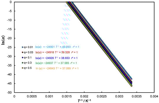
Figure 1.
Kinetic approach Equation (27) for for the assumed five heating rates.

Table 1.
Summary of calculated parameters of Equation (27) for five assumed heating rates and .
The numerical data summarized in Table 1 were verified using Equation (25). A graphical representation of the relationship obtained is presented in Figure 2. From the parameters of the obtained linear relationship:
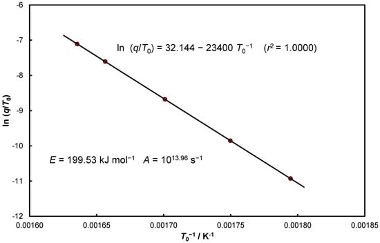
Figure 2.
Data presented in Table 1 in the Equation (25) coordinate system.
The activation energy and the pre-expotential factor were determined. As one can easily see, both determined parameters have slightly lower values than those used for calculations ().
The intercept value in Equation (32) is dependent on deviations of the activation energy and errors resulting from the observed variability of constants occurring in the kinetic functions.
Figure 3 presents the relationship (30) function D3 (Jander) but as R3: (R3).
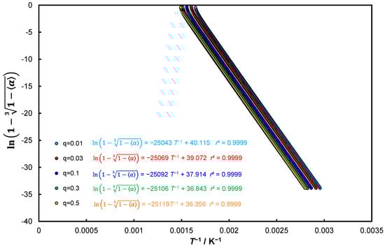
Figure 3.
The relationship for function D3 (Jander) as Equation (30) for five different heating rates.
Table 2 gives as an example the integration constant calculated according to Equation (14), but also comparatively Equations (16), (23) and (24) were used–all the mentioned formulas turn out to be equivalent.
Table 2.
Analysis of the kinetic function D3 as R3 by means of Equation (30), = 0.9999.
Thus, if this model accepts the coordinates then by force of facts Equation (25) remains unchanged in the analytical form of Equation (32).
Model D2 is very interesting because starting from infinitesimally small conversion degrees it goes from R1 through D1 to D2.
The consequences of the considerations for the assumed values of kinetic parameters and also provide an opportunity to analyze the isoconversion models.
The adopted methodology and the performed cycle of calculations indicate the possibility of extending the interpretation of Equation (9) it can be written in a form as KAS equation:
For each point with coordinates , an intercept is created: , and for the presented considerations the relationship has been assumed, what follows from considerations on Equation (13) and further ones. Figure 4 and Table 3 summarize the results of calculations for five different heating rates and for constant values of the conversion degree from 0.1 to 0.8.
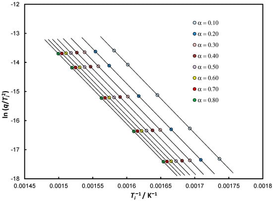
Figure 4.
Analysis of the theoretical data Equation (33) for the assumed values of the parameters of the Arrhenius law in isoconversion approach for eight positions of and five different heating rates.
Table 3.
Summary of calculation results for five different heating rates and for constant values of the conversion degree log A = 14.00 ln A = 32.236 r2 = 1.0000.
The data presented in Table 3 show that with the relative error below 0.02% we determine the activation energy and with a similar approximation, the pre-exponential factor . Despite the very small differences in values, we can derive KCE as an isoconversional effect :
The determined isokinetic temperature is higher than that provided in Table 1 even for heating rate , but more important is the fact that there appears a KCE that is statistically significant only for the isoconversion method.
The starting point of the calculation is the integration constant Equation (13), which initiates the possibility of confronting Equation (25), since formally in both cases . Considerations for simulated data show that the integration constant in Equations (14), (16), (19), (20) divides the kinetic data into a range of very low reaction/process rates from those corresponding to the higher temperature range and heating rates .
The KCE phenomenon, conventionally written as Equation (1) for is characterized by the fact that , so there is no simple way to relate to Equation (25) due to the variability of the ratio for . Note that even in the simplest kinetic case for the simulated R1 model this effect does not occur (Table 1). This fact is also confirmed by the data for model R3 (Table 2). A small increase in leads to a small decrease in , which contradicts the classical Arrhenius law [2], but is possible for physical processes. An example is the relationship between the two parameters of viscosity in the Arrhenius-like equation, such as the energy and the pre-exponential factor; see Figure 3b in [36].
At this stage of consideration, the importance of the initial temperature is confirmed, but there is not enough strong evidence to consider the isokinetic temperature as an undisputed quantity. From the data considered, it appears that .
3.2. Thermokinetic Analysis of Experimental Data
The starting point for kinetic considerations is Equation (13) and the assumption that (e.g., Anderson in [35]). This is supported by Equation (33) as well as the calculations presented in Table 4, although it will be necessary to verify this assumption. The calculations were based on the experimental data presented in [19] (Table 1a in [19]) for thermal dissociation of calcite in nitrogen under dynamic conditions.
Table 4.
Analysis of experimental data of thermal dissociation of calcite in nitrogen based on Equation (36)–Doyle approximation.
Bearing in mind the need to determine and , it was found that there are at least two possibilities to analyze the experimental data. The first option is to use the relationship:
while the second one uses the Doyle approximation for the intercept presented in [20]:
Equations (35) and (36) can be applied to isoconversional analyses in the form:
when Equation (37) is a special case of Equation (33) and Equation (38):
Experimental data of the thermal dissociation of calcite in nitrogen for the seven heating rates in the coordinate system of Equation (35) are presented in Figure 5.
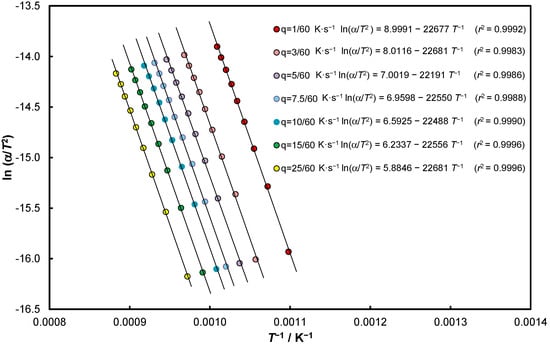
Figure 5.
Experimental data of thermal dissociation of calcite in nitrogen for seven heating rates and nines positions of α = const. in the coordinate system of Equation (35).
Equations (35)–(38) generate KCE and therefore the individual estimators were statistically verified–all relationships are significant with a probability of at least 99.99%. The relevant graphs are shown in Appendix A in Figure A1, Figure A2, Figure A3 and Figure A4, while whether the determined isokinetic temperatures can be considered authoritative will be presented later in the paper.
Equation (36) can be taken as analogous to Equation (13) for , by which, using Equation (19), the initial temperature can be determined. The obtained data were collected in Table 4, resulting in a confrontation similar to Equation (25)—Figure 6; this is a methodological comparison to Figure 2.
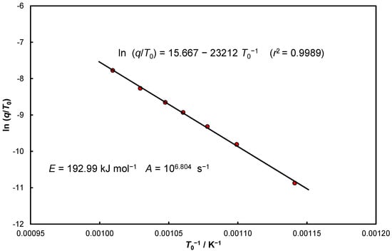
Figure 6.
Experimental data of the thermal decomposition of CaCO3 in nitrogen for seven heating rates in the coordinate system of Equation (25).
Based on the data summarized in Table 4, the following form of Equation (25) was determined:
from which and were calculated assuming (Figure 6).
The data from Table 4 [, as presented in Figure 6, confirm sufficient agreement with the data presented in the descriptions of Figure A1, Figure A2, Figure A3 and Figure A4, in particular, the value of both the activation energy and the frequency constant are close to the values given in the description of Figure A2. Obviously, the average values given in Table 4 are identical to those given in Figure A3a.
Continuing the discussion, it should be stated that the experimental data analyzed with Equation (36) are interpreted twice. Originally, according to Equation (36), the intercept being a Doyle approximation allows us to determine the frequency constant and the slope (the activation energy ). Hence, one obtains the KCE relation and further the isokinetic temperature . On the other hand, the intercept was interpreted according to Equation (19) by iteratively determining for each heating rate (Table 4).
Analytical determination of the coordinate for any kinetic data is complicated.
An interesting approach to the problem of determining this values is the use of a three-parameter equation [19,23,27,37]. Equation (40) allows a different approach than that proposed in the paper [38]:
after differentiation of Equation (40) relative to temperature, for and introducing Equation (10) we obtain:
and after multiplying both sides by and after ordering, we get:
The approximate methods can be used to determine the coordinates from the system of Equations (40) and (42).
After introducing Equations (42)–(40) for we obtain:
This way we can skip the tedious analytical determination of higher order derivatives referred to in [38] in order to calculate .
Table 5 summarizes the results of the experimental data analysis of the thermal decomposition of CaCO3 in nitrogen for seven heating rates using the three-parameter Equation (40). The initial temperature was determined by an iterative method using the system of Equations (40) and (42), which omits the complicated search for this temperature discussed in works [21,22,38].
Table 5.
Results of the analysis of experimental data on the thermal decomposition of CaCO3 in nitrogen for seven heating rates using the three-parameter Equation (40).
From the data presented in Table 5 it can be seen that with increasing heating rate the value of isokinetic temperature increases. According to the notation of Equations (10) and (42), it can be concluded that, with an increase in the heating rate, the reaction rate decreases monotonically. For the heating rates analyzed in this paper, the variation of the isokinetic temperature was less than 4% hence, all the data can be taken as one average value.
3.3. Consequences of the Analysis of Experimental Data
It should be noted that the relations are known in the literature as the temperature criterion [39] and are also discussed in works [40,41]. Equations (40) with (42), (43) are new elements in this respect and allow the determination of the isokinetic temperature.
As is known, the temperature criterion is valid for low conversion degrees. In the meantime, in this work, both in the part concerning model analyses (Figure 1) and experimental data of the thermal dissociation of calcite (Table 4), a linear relationship was obtained for all data, i.e., for the analyzed range of variation of conversion degree: as well for total range, as with its limitation, respectively.
While for model considerations this is acceptable, then for other more complicated solid decompositions after an initial stage with a high activation energy its value decreases with the conversion degree. The observations provided in [31] show that, in practice, different kinds of dependences of on can occur On the other hand, in Equations (35)–(38) with assumed Arrhenius parameters, the 0th order kinetics, was used.
Nevertheless, what distinguishes this work from previous considerations is the possible range of variation of to be analyzed, which omits the extremely important initial range for low conversion degree, as well as the end of the process. The first remark that comes to mind for comparison is the value of initial temperature–for the model it is equal to average , while for the experimental data (Figure A1, Figure A2, Figure A3 and Figure A4) it depends on the adopted kinetic function and, see Table 4, on average it is equal to (depending on ). When the experimental data for are analyzed using Equations (35) and (36), then . On the other hand, when we use isoconversion methods using Equations (37) and (38), we observe a wider range of variation , which authorizes the conclusion that isoconversion methods are characterized by a much weaker increase in the factor in relation to activation energy.
It should be noted that the parameters of the Arrhenius equation determined in this work from experimental data of the thermal decomposition of CaCO3 in nitrogen have similar values and are in agreement with the data collected in [35] (e.g., Anderson): , .
For the four cases resulting from Equations (35)–(38), the determined Arrhenius law parameters can be treated as average values, as evidenced by the very small standard deviations. Nevertheless, these small variations generate an observable KCE.
Comparing the results of the analysis of the model and experimental data, it is clear that, in both cases, the values of the activation energies are similar, however, the frequency constant calculated for the experimental data reaches a much lower value: , which makes the determined isokinetic temperatures take much higher values.
The kinetic Equations (35–38) were derived according to the presented model considerations, taking into account that the most important functional factor is the expression . However, since in order to create the single column matrix (26) the relation (9) was used, in the derived equations also the occurring variable had to be taken into account. Therefore, it can be assumed that going from Equations (35) and (36) this variable weaves into the free expression and only slightly changes the values of the estimators, remaining in accordance with KCE, i.e., the values of estimators and increase or decrease simultaneously.
4. Discussion
4.1. Isokinetics and Initial Temperature
Accepting the general thermokinetic Equation (11), it was proved that the great majority of kinetic equations can be generalized to a single relationship (13), which contains the most important component . Using the relationship (13) and forming the one-column matrix according to (26) one obtains a very practical for analysis of experimental data, Equations (27)–(31) with the intercept Equations (16), (19), (20), allowing us to determine the Arrhenius equation parameters and the initial (Equations (17) and (19)) or isokinetic temperature (Equation (1)).
We have complete agreement, when for the kinetic models presented in Table A1 the factors provided there will be used as proposed in [23,24]. Using Equation (25) and the single-column matrix we obtain the basis for inferring the substitutability of kinetic functions of thermal dissociation processes of the solid phase. By forming the single-column matrix for the assumed Arrhenius law parameters, we can reproduce these parameters using a modification of Equation (25), e.g., in the form of Equation (34)–Table 3. The situation is even more favorable for experimental data, which are illustrated in Figure 6.
Despite the observed variation of the initial temperature values with heating rate during analysis of both model and experimental data (Table 2, Table 4 and Table 5), the averaged values of and can be taken as correct. For these reasons, Equations (13) and (19), from which we determine the activation energy and the initial temperature, become significantly important.
In the case of experimental studies there is a possibility that Equations (13) and (19) will be valid in the whole experimentally determined range of conversion degree increase or in its selected range.
With the heating rate, the initial temperature increases, but the changing parameters of the Arrhenius law lead to a constant isokinetic temperature, .
The general forms of the Equation (13) can be reduced to the practical notation of Equation (24), which clearly indicates an extremely important element in thermogravimetric analysis for dynamic conditions, which is . Its determination is much more convenient and simpler, when we use the three-parameter Equation (40) along with Equations (42) and (43).
4.2. Isokinetic Temperature
As demonstrated by Lente in his book [42], the problem of determining kinetic parameters can lead to incorrect or unjustified quantities. Generally, justified considerations on the correctness of the determined parameters of the Arrhenius equation may undoubtedly include another element connected with it–the isokinetic temperature or compensation temperature , to which many works have been devoted, among others [4,21,41,42,43,44,45,46,47].
The temperature is determined by both Equation (1) and the classical KCE equation in the form, where intercept is expressed by the Arrhenius law, which formally makes it a tautology:
where:
When, in Equation (45), for each coordinate pair , the determined leads to then this is the “true” isokinetic temperature. The KCE in terms of (44) with (45) exhibits features of self-consistent equations. As will be shown further on, the fluctuation of the constant is relatively high despite .
Thus, it can be considered that this leads to a KCE called horizontal (isoconversional). According to the analyses presented in [43,44,45,46], the isoconversional KCE, characteristic of isoconversional methods, can be described as the statistical compensation effect [45] characterized by high isokinetic temperatures.
The fundamental problem, however, is whether the general notation of KCE (Equation (1)), and specifically in the form of Equation (34) and in Figure A1, Figure A2, Figure A3 and Figure A4, makes physicochemical sense for a significant statistical level, as defined by high value of determination coefficient.
For this purpose, two criteria: CQF (Compensation Quality Factor) and K according to [48,49] were used. The analytical distinction in the KCE (and EEC) relations in both physicochemical and statistical sense for high determination coefficients for a specific number of measurements was proposed. The K parameter can be called the position parameter.
For KCE assessment it is proposed:
For a probability of 99% [48]:
The meaning of the symbols and more methodological and interpretive details are included in Appendix A.
Starting from the evaluation of the veracity of the determined isokinetic temperature in Equation (34), an important issue is the determination of the temperature designated as . On the one hand, according to the data presented in Table 1, this is the average initial temperature , but simulation analyses were carried out starting from a temperature of 298 K. The average temperature for was taken as the temperature, i.e., .
For the first case using Equation (46) we get: and according to Equation (48) and Equation (47) , that is, the isokinetic temperature does not meet the criterion Equation (48). On the other hand, for the second version of we similarly obtain: and accept the physicochemical sense of the isokinetic temperature.
In this paper, the position parameter according to Equation (47) can be transformed to the form:
which makes it possible to carry out a position analysis according to the characters in the expression shown in brackets, i.e., , and The favourable case can be defined as the inequality: when , because , which means approaching to the initial temperature . When , then this condition [43] characterizes isoconversional methods relative to classical methods .
For simplicity, still assuming , this position parameter informs us about the relation between the isokinetic temperature and the range of tested temperatures in which it was determined, that is (Figure A5):
- (a)
- ;
- (b)
- ;
- (c)
- .
Case (c) can lead to excessively high isokinetic temperatures.
Returning to the calculations presented in Figure A1, Figure A2, Figure A3 and Figure A4, it can be noted that, despite statistically satisfactory significance levels, none of the items meet the CQF criteria. Thus, the isokinetic temperatures are experimentally determined quantities that do not satisfy the CQF in the physicochemical sense.
These considerations indicate that an important issue is the temperature range in which we observe KCE, and it is advantageous that it is as wide as possible. Due to the “quality” of KCE, when , then is closer to than to the final temperature of the reaction/process, which is relatively unfavorably much larger.
The criteria proposed in the works [48,49] may make it necessary to revisit many already published works.
4.3. Compensation Temperature
Eyring has derived an equation describing the reaction rate constant as a function of temperature and the free enthalpy of activation depending on the reaction mechanism limited by the formation of the active complex in gaseous phase [12]. The theses proposed in work [12] were adapted into the form of relations, in which the transmission coefficient and threshold energy distribution functions of the reactants were omitted [16,50,51,52,53,54] and only the “universal frequency term” was left [51]. This expression is directly proportional to the product of half equal to potential and kinetic energy [16]. The equation in its most common form is as follows:
where:
For the solid phase dissociation process following the reaction scheme: or and the value of the stoichiometric coefficient for the substrate the equation is known in the form of Equations (50) and (51) [53]. The use of the presented approach seems to be common for thermal dissociation of the solid phase, such as for the complete decomposition of calcium oxalate (CaC2O4·H2O) to CaO [16].
Using the concepts of a certain convergence between the Arrhenius and Eyring equations, from the equation we obtain:
while from the direct comparison of the constant rates we obtain:
Therefore, from Equation (51) and Equations (52) and (53) we determine the entropy of activation:
However, it should be noted that, despite the widespread acceptance of the presented comparison, there are premises which do not accept the concept of using the same set of input data [52].
On this basis, relationships between both activation thermodynamics and kinetics (parameters of the Arrhenius equation) are derived by taking the temperature of the maximum reaction rate as the activation temperature for dynamic conditions [53,54]:
Suppose that Equations (55) and (56) satisfy the EEC, with a slope called the compensation temperature (see Equation (2)), which directly follows from the second law of thermodynamics:
or:
By substituting Equations (55) and (56) into the form (57) and dividing the sides by , after transformation we get:
The sum of the last three components of Equation (59) is close to 0, which is evident either for or by taking the approximation: The derivation is also valid by taking , so it shows features of generality, and Equation (59) takes the form KCE:
The intercept in Equation (60) is:
and is the logarithmic form of Equation (50) containing the EEC expressed by Equation (58).
Ultimately, Equation (60) takes the typical form for KCE:
which means the identity of the isokinetic and compensating temperatures, The reverse possibility of transition from KCE (Equations (44) or (1)) to EEC (Equations (57) or (2)) can also be demonstrated.
From Equations (52) and (54) we extract the relevant Arrhenius parameters from the activation function at temperature :
and after inserting Equations (63) and (64) into the KCE structure we obtain:
Equation (65) satisfies the EEC expression of Equations (57) and (58). In addition, by substituting Equation (65) in the intercept: and using the Arrhenius equation for , we again obtain Equation (53).
The treatment of the presented considerations is a continuation of papers [1,4,5,20] and is based on the relationship between the parameters of the Arrhenius law and Eyring’s theory, from which it follows that the isokinetic temperature is equal to the compensation temperature. However, in the light of propositions to verify the physicochemical sense of the first mentioned [48,49] and one presented in Figure A1, Figure A2, Figure A3 and Figure A4 (see Appendix A), the determined quantities are reliable only from the point of view of statistical evaluation.
4.4. Isokinetic Temperature Again
In order to clarify the methodology of the experimental determination of isokinetic temperature, the parameters of the Arrhenius equation were used.
For the assumptions: , , Equation (22) determines the activation energy:
and using both Equation (19) and Equation (66) we obtain:
The data illustrated in Figure A1 and according to Equations (66) and (67) were combined with an additional coordinate considered in this work as a reference in [35] (e.g., Anderson) and are presented in Figure 7.
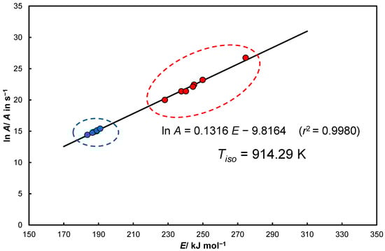
Figure 7.
Typical KCE plot representing two groups of Arrhenius parameters pairs that form one IE.
The determined activation energies presented in Figure 7 form two resultant groups, in fact, they are combined in the form of one simple KCE. Results of the scoring method (much higher values–red) can be classified as quasi-isoconversional . On the other hand, values that are lower (blue) or close to the reference data (E = 191 kJ/mol, lnA = 15.4/ A in s−1) [35], e.g., Anderson) are determined for individual heating rate-dependent curves by the Coats−Redfern equation for a range of changes .
For the data presented in Figure 7 for Equation (46) and , and temperatures: , (for [5]) and setting up for and probability at least 99% (sl = 0.01) (Equation (48)):
and from Equation (49):
This result shows the reliability of the determined isokinetic temperature, which is ahead of the range of tested temperatures . It therefore has the character of an extrapolated quantity.
4.5. Summary of Equations for Experimental Data
The resolution of the significance of the determined temperatures is described by three equations:
- typical KCE equation (Figure 7):
- slope in Equation (57) provided in [43] concerning calcite dissociation from different references:
- from the linear relationship between the parameters of the three-parameter equation, Table 5 (slope in Equation (70)):
However, according to Equation (45), for the constant temperature provided in Equation (68) , a relatively large range is obtained: .
In turn, we calculate only one compensation constant: from Equation (61) for the constants given in Equation (69). The value of this constant is much higher than the calculated average value of the isokinetic constant . Thus, the intercept in KCE is literally a quantity that averages a wide range of variation in the kinetic constant at the isokinetic point.
Synoptic Figure 8 explains the discrepancy between and the experimentally obtained KCE. The analytical considerations take into account a very wide range of conversion degree variations up to the co-ordinate while the research scope focuses on higher conversion degrees. By making selections in the base of single column matrix towards , the slope, or activation energy, increases.
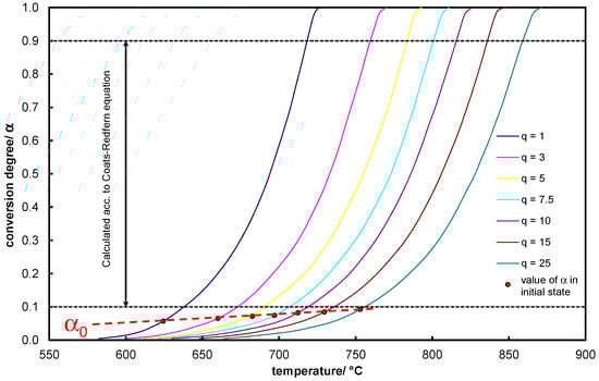
Figure 8.
An illustrative comparison of using experimental data to determine the KCE equations.
According to Table 6, the relationships between the obtained temperature quantities are not very different from each other. The identity between and is not confirmed (according to Equation (62)), and in turn approaches [19]. The initial temperatures are consistent for the snapshots given in Table 4 and Table 5 and, as it were, in their interval “absorb” the isokinetic temperature of Equation (68), which fulfills the indicator criterion of CQF, K [48,49].
Table 6.
Summary of temperatures determined for experimental data ( = 1172.4 K [19]).
The experimental data in terms of Equations (44) and (68) form a sequence of inequalities , while the exact isokinetic temperature is calculated from the formula: . In the correlation calculus using the ratio for the exact calculation of was emphasized in the work [43], by which the accuracy of the numerical values between KCE and EEC (Equations (68) and (69)) should be distinguished, which was also pointed out in [55].
However, when too large a fluctuation of the assumed constancy of is observed, it becomes necessary to carry out selection according to the proposal of Perez-Benito et al. [5,20]. The simplest approach is represented by inequality (71):
where corresponds to temperature in Equations (55) and (56) and is determined in [20] as a working temperature.
According to the findings of (71), the inequality is satisfied by Equations (68) and (69) in relation to the temperature of the maximum reaction rate, equal to for a heating rate of 25 K/min (Table 5). In contrast, Equations (10) and (70) are closer to the definition of initial temperature. These findings remain consistent with the proposal of [43].
Following the concepts already used in Equations (46)−(49), the physicochemical sense of isokinetic and compensation temperature, which according to Equation (62) should be the same, it is most advantageous to verify in two steps based on the work [48,49] for statistically significant correlations.
It was proved experimentally that for chemical reactions of four chemically similar compounds (dissociation of hexacene dimers) the Eyring plot indicates the fact of occurrence of several times in a narrow temperature range [56].
EEC expands our understanding of the little-studied quantitative aspects of organic reactions. Experimental evidence of its physical reality in a number of cross reaction series is considered through non-catalytic and pyridine-catalyzed reactions of aryloxiranes with organic acids of various classes. In the context of the compensation effect, there are transitions from one state of reaction systems in which the enthalpy term of the free activation energy acquires a zero value (, ), to another, in which the contribution to the free energy of activation of the entropy term disappears (, ) [57]. Mentioned in parentheses is that the thermodynamic states of the activation process are included in Equation (58).
On the other hand, from a physicochemical point of view, a very interesting example is presented in [46] concerning temperature programmed desorption (TPD), when the surface coverage decreases with increasing temperature. Analyzing this phenomenon as a reversible process, while the isosteric heat of adsorption–once the entropy is determined–leads to EEC [6], the constant surface coverage condition is not respected–as is the case in isothermal sorption kinetic measurements–we observe a rather large scatter in terms of KCE [47].
4.6. Some Remarks to All the Elements
For dynamic conditions, the equation in differential form, Equation (8), is commonly recognized as the starting point for consideration. If the approximate form of the solution of Equation (8), referred to by the authors as the Coats−Redfern equation (Equation (9)), interacts with this equation, it leads to Equation (13). This equation has an identical mathematical structure, independent of the heating rate and pre-exponential factor. The consequences of analyzing the adoption of specific analytical forms of the integration constant open up new possibilities for comparison of the Arrhenius parameters obtained through different paths, including Vyazovkin’s, discussed in detail in the book [31]. In contrast to isoconversion concepts, in this work one still stays with the classical variant and for this possibility and for simulated “in silico” data the very important significance of the coordinate is presented, thanks to which Equation (25) reproduces the activation energy and also the constant . For many models, can be calculated or simply ignored.
In relation to the proposal to determine the “elbow” point coordinate, based on the knowledge of higher order derivatives [38], the methodology has been simplified, which boils down to determining the isokinetic temperature from the constant in Equation (19) and calculating the initial transformation step from Equation (27) or (40).
On the other hand, consideration of simulated data does not provide a basis to demonstrate the existence of the KCE, which appears for experimental data. It is necessary not only to verify it statistically, but also using the CQF and K indicators via Equations (46)−(49) to give the isokinetic temperature a physicochemical sense.
In the association of works [5,20,21,43], the experimentally determined considered temperatures form a sequence, where denotes the thermodynamically determined equilibrium temperature of the reaction (Equation (6)), sometimes also called the inversion temperature:
The current work proved that the temperatures and are theoretically equal (compare Equations (44) and (62)), while the temperature sequence given in Equation (72) follows from many factors. These are: sample quality (mass, degree of purity, moisture content, crystalline/amorphous form, analysis conditions: isothermal/dynamic, heating rate, atmosphere, flow, reactor type) and workshop issues (variation of , calculation techniques, distinguishing variants: or ). In light of these considerations, the isokinetic temperature is of lesser reliability than the initial temperature or even the compensation temperature , which is implicit in the kinetic relationship.
As noted in [52], Equation (69) is derived from various sources, and Equation (68) is composed of correlation and point analysis–both equations involve the same reaction/process of thermal decomposition of calcite.
The omitted analysis of Equation (3) in conjunction with Equation (2) was hinted at in the paper [43].
5. What’s Next?
From the point of view of the equations used, the starting point is the generally used Equation (8) for dynamic conditions and its most commonly used approximate Coats−Redfern solution (Equation (9)). The relation of Equations (8) with (9) leads to the differential Equation (11) with the analytical solution Equation (13). The condition of Equation (10) allows the determination of several equivalent forms of the integration constant in Equations (23) and (24). The final form of Equation (25) determines the activation energies using the heating rate (q) and initial temperature (T0). In further steps, a new way of determining the coordinates [T0;α0] in Equations (40)−(43) is proposed. Further procedures use the relations of KCE, EEC and their constant characteristic temperatures against a narrowly variable initial temperature (T0).
6. Conclusions
1. The relationship between KCE and EEC is mutually possible and it has been shown that the relationship theoretically should occur. In light of these considerations, the isokinetic temperature is of less reliability than the initial temperature or even the compensation temperature . The analysis for the same data of the thermal dissociation of calcite in nitrogen comes down to a sequence of temperatures .
2. The effect of the generally known Coats−Redfern solution influence on the differential kinetic equation for dynamic conditions (Equation (8)) and on the resulting isokinetic mathematical forms (Equation (13)) has been used. For in silico and experimental data in the case of thermal dissociation of simple solid chemical compounds, a relationship between the initial temperature and the heating rate has been demonstrated, which enables the determination of the Arrhenius equation parameters. An analytical way of determining the coordinate based on the three-parameter equation considering the derivative at temperature , has been proposed.
3. In solid-phase thermokinetic analysis, isokinetic relationships have been known for years. Equation (13) is independent of the heating rate and the activation energy is in turn invariant with the conversion degree. The integration constant in this equation can be expressed analytically in various ways. The possibility of its determination by quantities included in the coordinate when const, has been demonstrated. This type of viewpoint presents a different approach from the isoconversion methodology, for which is very often observed.
4. Using the parameters CQF and K as in [48,49], it has been shown that KCE in the physicochemical sense favors wide ranges of parameter variations of the Arrhenius law. The CQF index determines the reliability of even a very high probability of a linear relationship of the KCE. On the other hand, the position parameter K, assuming , indicates that, for −1 ≤ K ≤ 1, the isokinetic temperature is within the range of tested temperatures and for the other values it has an extrapolative character.
Author Contributions
All authors contributed to the study conception and design. The first draft of the manuscript was written by A.M. and all authors commented on previous versions of the manuscript. A.M. Literature research, material preparation, data collection and analysis, writing the paper. T.R. Data collection and analysis, calculations, writing the paper, data visualization, discussion. R.B. Calculation and data verification, discussion, manuscript formatting and text correction. All authors have read and agreed to the published version of the manuscript.
Funding
This research received no external funding.
Data Availability Statement
Not applicable.
Conflicts of Interest
The authors declare no conflict of interest.
Nomenclature
| coefficients of the three-parametric Equation (40), in K, | |
| A | pre-exponential factor, s−1, |
| B= | ratio of Boltzmann to Planck’s constant, |
| C | integrals constant, |
| CQF | Compensation Quality Factor as in [48,49], |
| E | activation energy, J mol−1, |
| kinetics functions, | |
| ΔG | free enthalpy, Jmol−1 |
| H = 6.62607×10⁻³⁴ Js, | Planck constant |
| free enthalpy of activation in temperature, Equation (58), J mol−1, | |
| ΔH | enthalpy, Jmol−1, |
| k, | rate constant and dependent on T, s−1, |
| = 1.38065·10−23 JK−1 | Boltzmann constant, |
| average value of the isokinetic constant, s−1, | |
| K | position of coalescence as in [49], or position parameter, |
| m | coefficients, |
| n | exponent, |
| N | number of data, |
| p | pressure, Pa, |
| coefficients of linear or multiple determination, | |
| R = 8.314 J (mol·K)−1 | universal gas constant, |
| q | heating rate, K s−1, |
| sl | significance level, |
| ΔS | entropy, J(mol*K)−1, |
| T | absolute temperature, K, |
| T0 | initial temperature, K, |
| x | E/RT, |
| α | conversion degree, 0 < α ≤ 1, |
| single column matrix, | |
| β, γ | constants in Equations (1)–(3), |
| ν | stoichiometric coefficient. |
| Subscripts: | |
| c | compensation, |
| eq | equilibrium, |
| low, high, hm | relate to mean values of initial and final temperatures and their harmonic mean respectively, |
| i | ith value, |
| Iso | isokinetic values, |
| m | maximum of rate reaction/process, |
| Superscripts | |
| + | activation functions, |
| * | auxiliary quantity, Equations (A1), (A2), |
| g, s | gas, solid, |
| standard condition | |
| Abbreviations | |
| EEC | Enthalpy−Entropy Compensation, |
| ICTAC | International Confederation for Thermal Analysis and Calorimetry, |
| KAS | Kissinger−Akahira−Sunose equation, |
| KCE | Kinetic Compensation Effect (also IKR, IE), |
| TPD | Temperature Programmed Desorption. |
Appendix A
Table A1.
List of kinetic functions as in [31] and approximation of the first term in Equation (14) (.
Table A1.
List of kinetic functions as in [31] and approximation of the first term in Equation (14) (.
| Code | ||||
|---|---|---|---|---|
| P4 | ||||
| P3 | ||||
| P2 | ||||
| P2/3 | ||||
| D1 | ||||
| F1 | ||||
| A4 | ||||
| A3 | ||||
| A2 | ||||
| D3 | ||||
| R3 | ||||
| R2 | ||||
| D2 |
* Maclaurin expansion was used, for model D3–after squaring. Stopped at the first term of the equation.
- Analysis of KCE for Experimental Data
The KCE resulting from the analysis of the experimental data on the thermal dissociation of calcite in nitrogen is presented in Figure A1. While Figure A1a presents the KCE resulting from the analysis of data according to Equation (35) for seven different heating rates. Figure A1b presents the KCE for six different heating rates, omitting data for q = 1/60 K·s−1.

Figure A1.
KCE for experimental data of thermal dissociation of calcite in nitrogen: (a) source: Equation (35), N = 7 heating rates, 1014.7 K, E = 187.45 ± 1.34 kJ·mol−1, lnA = 14.88 ± 0.16 (A in s−1), sl = 0.0(3)14; (b) source: Equation (35), N = 6 heating rates (data for q = 1/60 K·s−1 is omitted), 949.5 K, E = 187.27 ± 1.37 kJ·mol−1, lnA = 14.87 ± 0.17, (A in s−1). sl = 0.0(4)19.
Despite the small variability of the parameters of the Arrhenius law, they meet the KCE at a sufficient level of significance. The average results provided in the description of Figure A1 are consistent with the data presented by Anderson [21] for the 0th order kinetics (E = 191 kJ·mol−1, lnA = 15.4/A in s−1).
The average values obtained with the use of the kinetic function (37) are slightly different, as presented in Figure A2.

Figure A2.
KCE for experimental data of thermal dissociation of calcite in nitrogen: (a) source: Equation (37), N = 9 positions α = const., 1074.0 K, E = 192.45 ± 0.90 kJ·mol−1, lnA = 15.49 ± 0.10 (A in s−1), sl = 0.0(5)8; (b) source: Equation (37), N = 8 positions α = const. (data for α = 0.1 is omitted), 1246.8 K, E = 192.24 ± 0.71 kJ·mol−1, lnA = 15.46 ± 0.07 (A in s−1), sl = 0.0(4)8.
In relation to the analysis presented in Figure A2. the isoconversional approach of Equation (37) for the average values of and is not too much of an outlier and falls within the ranges presented in [21] but with an unsatisfactory coefficient of determination. However, it should be noted that the calculated isokinetic temperatures differ significantly depending on the data selection method. In the case of experimental research, when we analyze only the available range of increase in the conversion rate from temperature (here a different type of KCE is observed for the constant heating rate analyses and a different type for the isoconversional method. The position presented in [5] is thus confirmed.
Figure A3 and Figure A4 show the KCE resulting from the analysis of experimental data of thermal dissociation of calcite in nitrogen from Equations (36) and (38).

Figure A3.
KCE for experimental data of thermal dissociation of calcite in nitrogen: (a) source: Equation (36), 9 positions for α = const and N = 7 heating rates, = 1052.2 K, E = 204.46 ± 1.44 kJ·mol−1, lnA = 15.90 ± 0.17 (A in s−1), sl = 0.0(3)15; (b) source: Equation (36), 9 positions for α = const and N = 6 heating rates (data for q = 1/60 K·s−1 is omitted) = 1060.6 K, E = 204.48 ± 1.56 kJ·mol−1, lnA = 15.92 ± 0.18 (A in s−1), sl = 0.0(4)2.

Figure A4.
KCE for experimental data of thermal dissociation of calcite in nitrogen: (a) source: Equation (38), 7 heating rates and N = 9 positions for α = const, = 1264.4 K, E = 209.45 ± 1.01 kJ·mol−1, lnA = 16.46 ± 0.10 (A in s−1), sl = 0.0(5)1; (b) source: Equation (38), 7 heating rates and N = 8 positions for α = const (α = 0.1 is rejected, = 1298.4 K, E = 209.35 ± 1.04 kJ·mol−1, lnA = 16.45 ± 0.10 (A in s−1), sl = 0.0(5)4.
- Physicochemical sense of isokinetic temperature
Temperature in Equation (46) follows from implication, when:
In Equation (48), the quantity 0.29 ≈ 1– is the CQF threshold for an infinite number of N measurements.
The individual temperatures denote the test temperature interval: is the arithmetic mean of the initial temperatures, is the mean temperature of the end of the interval and is the harmonic mean of the temperatures . .
For Equation (46) limit values are observed:
- in the simplest variant: .
In turn, the position parameter K indicates the location of relative to the range of temperatures used–Figure A5.
Always thus in Equation (49) K = 0 is parallel when (Equation (47).

Figure A5.
Arrhenius plot with indication of location of in relation to the temperatures analyzed, taking into account data from [48,49] only for the case where r2 = 1.
References
- Pan, A.; Biswas, T.; Rakshit, A.K.; Moulik, S.P. Enthalpy-Entropy Compensation (EEC) effect: A revisit. J. Phys. Chem. 2015, 119, 15876–15884. [Google Scholar] [CrossRef]
- Mianowski, A.; Radko, T. Analysis of isokinetic effect by means of temperature criterion in coal pyrolysis. Pol. J. Appl. Chem. 1994, 38, 395–405. [Google Scholar]
- Freed, K.F. Entropy-Enthalpy Compensation in chemical reactions and adsorption: An exactly solvable model. J. Phys. Chem. B 2011, 115, 1689–1692. [Google Scholar] [CrossRef]
- Liu, L.; Guo, Q.-X. Isokinetic relationship, isoequilibrium relationship, and enthalpy-entropy compensation. Chem. Rev. 2001, 101, 673–695. [Google Scholar] [CrossRef] [PubMed]
- Perez-Benito, J.F. Some tentative explanations for the enthalpy–entropy compensation effect in chemical kinetics: From experimental errors to the Hinshelwood-like model. Mon. Chem.-Chem. Mon. 2013, 144, 49–58. [Google Scholar] [CrossRef]
- Mianowski, A.; Urbańczyk, W. Enthalpy–entropy compensation for isosteric state adsorption at near ambient temperature. Adsorption 2017, 23, 831–846. [Google Scholar] [CrossRef][Green Version]
- Pan, A.; Kar, T.; Rakshit, A.K.; Moulik, S.P. Enthalpy−Entropy Compensation (EEC) Effect: Decisive Role of Free Energy. J. Phys. Chem. B 2016, 120, 10531–10539. [Google Scholar] [CrossRef]
- Movileanu, L.; Schiff, E.A. Entropy–enthalpy compensation of biomolecular systems in aqueous phase: A dry perspective. Mon. Chem. -Chem. Mon. 2013, 144, 59–65. [Google Scholar] [CrossRef] [PubMed]
- Dutronc, T.; Terazzi, E.; Piguet, C. Melting temperatures deduced from molar volumes: A consequence of the combination of enthalpy/entropy compensation with linear cohesive free-energy densities. RSC Adv. 2014, 4, 15740–15748. [Google Scholar] [CrossRef]
- Compendium of Chemical Terminology, Gold Book, Version 2.3.3, IUPAC. 2014. Available online: https://goldbook.iupac.org (accessed on 1 June 2020).
- Starikov, E.B. Bayesian Statistical Mechanics: Entropy-Enthalpy Compensation and Universal Equation of State at the Tip of Pen. Front. Phys. 2018, 6, 2. [Google Scholar] [CrossRef]
- Eyring, H. The Activated Complex in Chemical Reactions. J. Chem. Phys. 1935, 3, 107–115. [Google Scholar] [CrossRef]
- Laidler, K.J.; King, M.C. The Development of Transition-State Theory. J. Phys. Chem. 1983, 87, 2657–2664. [Google Scholar] [CrossRef]
- Rooney, J.J. An explanation of isokinetic temperature in heterogeneous catalysis. Catal. Lett. 1998, 50, 15. [Google Scholar] [CrossRef]
- Rooney, J.J. Isokinetic temperature and the compensation effect in catalysis. J. Mol. Catal. A Chem. 1998, 133, 303–305. [Google Scholar] [CrossRef]
- Błażejowski, J.; Zadykowicz, B. Computational prediction of the pattern of thermal gravimetry data for the thermal decomposition of calcium oxalate monohydrate. J. Therm. Anal. Calorim. 2013, 113, 1497–1503. [Google Scholar] [CrossRef]
- Yin, C.; Du, J. The power-law reaction rate coefficient for an elementary bimolecular reaction. Phys. A Stat. Mech. Appl. 2014, 395, 416–424. [Google Scholar] [CrossRef]
- Aquilanti, V.; Coutinho, N.D.; Carvalho-Silva, V.H. Kinetics of low-temperature transitions and a reaction rate theory from non-equilibrium distributions. Phil. Trans. R. Soc. A 2017, 375, 20160201. [Google Scholar] [CrossRef]
- Mianowski, A.; Urbańczyk, W. Isoconversional methods in thermodynamic principles. J. Phys. Chem. A 2018, 122, 6819–6828. [Google Scholar] [CrossRef]
- Perez-Benito, J.F.; Alburquerque-Alvares, I. Kinetic compensation effect: Discounting the distortion provoked by accidental experimental errors in the isokinetic temperature value. Mon. Chem. -Chem. Mon. 2020, 151, 1805–1816. [Google Scholar] [CrossRef]
- Lyon, R.E. Isokinetics. J. Phys. Chem. A 2019, 123, 2462–2499. [Google Scholar] [CrossRef] [PubMed]
- Lyon, R.E. Isokinetic analysis of reaction onsets. Thermochim. Acta 2022, 708, 179117. [Google Scholar] [CrossRef]
- Mianowski, A. Thermal dissociation in dynamic conditions by modeling thermogravimetric curves using the logarithm of conversion degree. J. Therm. Anal. Calorim. 2000, 59, 747–762. [Google Scholar] [CrossRef]
- Mianowski, A.; Siudyga, T. Influence of sample preparation on thermal decomposition of wasted polyolefins-oil mixtures. J. Therm. Anal. Calorim. 2008, 92, 543–552. [Google Scholar] [CrossRef]
- Órfão, J.J.M. Review and evaluation of the approximations to the temperature integral. AIChE J. 2007, 53, 2905–2915. [Google Scholar] [CrossRef]
- Carrero-Mantilla, J.I.; Rojas-González, A.F. Calculation of the temperature integrals used in the processing of thermogravimetric analysis data. Ing. Compet. 2019, 21, 7450. [Google Scholar] [CrossRef]
- Mianowski, A.; Baraniec, I. Three-parametric equation in evaluation of thermal dissociation of reference compound. J. Therm. Anal. Calorim. 2009, 96, 179–187. [Google Scholar] [CrossRef]
- Málek, J. The kinetic analysis of non-isothermal data. Thermochim. Acta 1992, 200, 257–269. [Google Scholar] [CrossRef]
- Senum, G.; Yang, R. Rational approximations of the integral of the Arrhenius function. J. Therm. Anal. 1977, 11, 445–447. [Google Scholar] [CrossRef]
- Starink, M.J. The determination of activation energy from linear heating rate experiments: A comparison of the accuracy of isoconversion methods. Thermochim. Acta 2003, 404, 163–176. [Google Scholar] [CrossRef]
- Vyazovkin, S. Isoconversional Kinetics of Thermally Stimulated Process; Springer International Publishing: Cham, Switzerland, 2015. [Google Scholar] [CrossRef]
- Budrugeac, P. Comparison between model-based and non-isothermal model-free computational procedures for prediction of converion-time curves of calcium carbonate decomposition. Thermochim. Acta 2019, 679, 178322. [Google Scholar] [CrossRef]
- Dahme, A.; Junker, H.J. Die Reaktivität von Koks gegen CO2 im temperaturbereich 1000–1200 °C. Brennst Chem. 1955, 36, 193–199. (In German) [Google Scholar]
- Balart, R.; Garcia-Sanoguera, D.; Quiles-Carrillo, L.; Montanes, N.; Torres-Giner, S. Kinetic analysis of the thermal degradation of recycled acrylonitrile-butadienie-styrene by non-isothermal thermogravimetry. Polymers 2019, 11, 281. [Google Scholar] [CrossRef] [PubMed]
- Brown, M.E.; Maciejewski, M.; Vyazovkin, S.; Nomen, R.; Sempere, J.; Burnham, A.; Opfermann, J.; Strey, R.; Anderson, H.L.; Kemmler, A.; et al. Computational aspects of kinetic analysis: Part A: The ICTAC kinetics project-data, methods and results. Thermochim. Acta 2000, 355, 125–143. [Google Scholar] [CrossRef]
- Messaâdi, A.; Dhouibi, N.; Hamda, H.; Belgacem, F.B.M.; Adbelkader, Y.H.; Ouerfelli, N.; Hamzaoui, A.H. A new equation relating the viscosity Arrhenius temperature and the activation energy for some Newtonian classical solvents. J. Chem. 2015, 2015, 163262. [Google Scholar] [CrossRef]
- Mianowski, A.; Urbańczyk, W. Thermal dissociation in terms of the second law of chemical thermodynamics. J. Therm. Anal. Calorim. 2016, 126, 863–870. [Google Scholar] [CrossRef][Green Version]
- Satopää, V.; Albrecht, J.; Irwin, D.; Raghavan, B. Finding a “knedle” in a haustack: Detecting knee points in system behavior. In Proceedings of the 31st International Conference on Distributed Computing Systems Workshop, Minneapolis, MN, USA, 20–24 June 2011. [Google Scholar] [CrossRef]
- Szarawara, J.; Kozik, C. Application of a new method for studies on the area of selected heterogeneous processes (Zastosowanie nowej metody badania obszaru do wybranych procesów heterogenicznych). Chem. Stosow. 1976, 20, 45–69. (In Polish) [Google Scholar]
- Mianowski, A.; Radko, T. The possibility of identification of activation energy by means of the temperature criterion. Thermochim. Acta 1994, 247, 389–405. [Google Scholar] [CrossRef]
- Mianowski, A.; Siudyga, T.; Polański, J. Szarawara-Kozik’s temperature criterion in the context of three-parameter equation for modeling ammonia or methanol decomposition during heterogenous catalysis. Reac. Kinetic Mech. Cat. 2018, 125, 493–504. [Google Scholar] [CrossRef]
- Lente, G. The fallacy of the isokinetic temperature. In Deterministic Kinetics in Chemistry and Systems Biology. The Dynamics of Complex Reaction Networks; Springer: New York, NY, USA, 2015; pp. 121–122. [Google Scholar] [CrossRef]
- Mianowski, A.; Radko, T.; Siudyga, T. Kinetic compensation effect of isoconversional methods. Reac. Kinetic Mech. Cat. 2020, 132, 37–58. [Google Scholar] [CrossRef]
- Norwisz, J.; Musielak, T. Compensation law again. J. Therm. Anal. Calorim. 2007, 88, 751–755. [Google Scholar] [CrossRef]
- Barrie, P.J. The mathematical origins of the kinetic compensation effect: 1. The effect of random experimental errors. Phys. Chem. Chem. Phys. 2012, 14, 318–326. [Google Scholar] [CrossRef] [PubMed]
- Barrie, P.J. The mathematical origins of the kinetic compensation effect: 2. The effect of systematic errors. Phys. Chem. Chem. Phys. 2012, 14, 327–336. [Google Scholar] [CrossRef] [PubMed]
- Mianowski, A.; Marecka, A. The isokinetic effect as related to the activation Energy for the gases diffusion in coal at ambient temperatures. Part II. Fick’s diffusion and isokinetic effect. J. Therm. Anal. Cal. 2009, 96, 495–499. [Google Scholar] [CrossRef]
- Griessen, R.; Boelsma, C.; Schreuders, H.; Broedersz, C.P.; Gremaud, R.; Dam, B. Single Quality Factor for Enthalpy-Entropy Compensation, Isoequilibrium and Isokinetic Relationships. Chemphyschem 2020, 21, 1632–1643. [Google Scholar] [CrossRef]
- Griessen, R.; Dam, B. Simple Accurate Verification of Enthalpy-Entropy Compensation and Isoequilibrium Relationship. Chemphyschem 2021, 22, 1774–1788. [Google Scholar] [CrossRef] [PubMed]
- Piskulich, Z.A.; Oluwaseun, O.M.; Thompson, W.H. Activation Energies and Beyond. J. Phys. Chem. A 2019, 123, 7185–7194. [Google Scholar] [CrossRef] [PubMed]
- Carvalho-Silva, V.H.; Aquilanti, V.; de Oliveira, H.C.B.; Mundim, K.C. Deformed Transition-State Theory: Deviation from Arrhenius Behavior and Application to imolecular Hydrogen Transfer Reaction Rates in the Tunneling Regime. J. Comput. Chem. 2016, 1, 11. [Google Scholar] [CrossRef] [PubMed]
- Khrapunov, S. The Enthalpy-entropy Compensation Phenomenon. Limitations for the Use of Some Basic Thermodynamic Equations. Curr. Protein Pept. Sci. 2018, 19, 1088–1091. [Google Scholar] [CrossRef]
- Olszak-Humienik, M.; Możejko, J. Eyring parameters of dehydration processes. Thermochim. Acta 2003, 405, 171–181. [Google Scholar] [CrossRef]
- Bigda, R.; Mianowski, A. Influence of heating rate on kinetic quantities of solid phase thermal decomposition. J. Therm. Anal. Calorim. 2006, 84, 453–465. [Google Scholar] [CrossRef]
- Lente, G.; Fábián, I.; Poë, A.J. A common misconception about the Eyring equation. New J. Chem. 2005, 29, 759–760. [Google Scholar] [CrossRef]
- Nakamura, S.; Sakai, H.; Fuki, M.; Kobori, Y.; Tkachenko, N.V.; Hasobe, T. Enthalpy−Entropy Compensation Effect for Triplet Pair Dissociation of Intramolecular Singlet Fission in Phenylene Spacer-Bridged Hexacene Dimers. J. Phys. Chem. Lett. 2021, 12, 6457–6463. [Google Scholar] [CrossRef] [PubMed]
- Shpanko, I.V.; Sadovaya, I.V. Enthalpy–Entropy Compensation in Reactions of Oxirane Ring Opening. Russ. J. Phys. Chem. A 2022, 96, 2307–2317. [Google Scholar] [CrossRef]
Disclaimer/Publisher’s Note: The statements, opinions and data contained in all publications are solely those of the individual author(s) and contributor(s) and not of MDPI and/or the editor(s). MDPI and/or the editor(s) disclaim responsibility for any injury to people or property resulting from any ideas, methods, instructions or products referred to in the content. |
© 2023 by the authors. Licensee MDPI, Basel, Switzerland. This article is an open access article distributed under the terms and conditions of the Creative Commons Attribution (CC BY) license (https://creativecommons.org/licenses/by/4.0/).