Electricity Load Lost in the Largest Windstorms—Is the Fragility-Based Model up to the Task?

Abstract

Most existing models for estimating electric system impacts from windstorms tend to have detailed representation only for the electric or only for the meteorological system. As a result, there is little evidence on how models with detailed electric systems and realistic wind gust field representations would perform in different windstorm cases. This work explores the evidence for the ability of such a fragility-based model to generate realistic spatiotemporal lost load profiles for the most impactful windstorm cases in Finland. The literature review shows multiple driving factors for windstorm impacts that are difficult to assess analytically, and similarities between the most impactful windstorms. All the available interruption data for thirteen years were analyzed, with their grouping by individual storm and calm periods. The fixing of time distribution fits for these periods show most faults as being within the 20% uncertainty bounds of the severity-dependent distribution trendlines. The medium-voltage electricity grid impact model with national coverage was applied for the three most impactful and most recent windstorm cases, with the model calibrated for one case. The generated spatiotemporal lost load profiles in all cases recreate historic profiles within the similar error margins of approximately 20%.

1. Introduction

Extreme weather events, with windstorms at the forefront, are responsible for a large share of the major blackouts globally [1]. Windstorms are strong, low-pressure systems, and are the type of storm that forms at the mid-latitudes, also known as an extratropical cyclone, driven by horizontal temperature gradients. Windstorms produce strong winds over areas that can span several hundred to several thousand kilometers in diameter [2]. In Finland, windstorms are the dominant source of electricity interruptions, with a small number of the strongest windstorms responsible for the majority of all electricity supply interruptions [3]. These interruptions are costly, but the same is also true for many measures to reduce electricity interruptions [4]. In other words, there is a risk of both significant under- and over-adaptation [5]. Thus, the economically sound development of the electricity system and of the most vulnerable sectors to electricity interruptions depends on knowledge of the impacts of major windstorms on the planned grids and electricity supply going through them. This knowledge can be obtained via the modeling of weather and electric grid systems, to generate spatiotemporal wind gust fields and, with them, a spatiotemporal lost load (LL) profile. Such modeling includes a multitude of relevant weather and electricity system aspects that can be represented in a multitude of ways, and at different levels of sophistication.

Electricity system representation differs by both the presence and detail of various system aspects. The simplest representations include only the spatial distribution of certain system components, and their possibility of faults. Examples of such representations are present in models using machine learning methods that link wind gusts to outages defined as the disconnections of transformers [6] or consumers [7]. Other machine learning models account for the spatial distribution of multiple grid components (e.g., [8,9]). More comprehensive electricity system representations can be found in analytical models that link the wind gust speed with faults in individual components, via so-called fragility functions. Fragility-based models include various combinations of additional aspects, with the major ones being the grid topology, component repair, and consumption. The grid topologies found in fragility-based wind impact models range from standard test systems (e.g., [10]) and simplified transmission grids (e.g., [11]) for which a significant portion of data is publicly available, to distribution grids generated from proxy data (e.g., [12]), as their actual topology data are typically unavailable [13]. An account of component repairs enables the modeling of the temporal dimension of disruption. The works that do account repairs range from repair times being a product of a component-specific constant and a random number [14], to modeling repair staff constraints [15]. The impact assessment in terms of the number of faults (NoFs) provides valuable information for the allocation of repair assets (e.g., [16]), and the means of studying the component importance in cascading failures [17]. However, cost considerations require an account of consumption, as the electricity supply in a sufficiently long disruption is more valuable than the infrastructure enabling it. The account of consumption without a temporal dimension is relatively straightforward (e.g., [18]), while a temporal consumption account requires the generation of synthetic (i.e., real-like) consumption profiles, which is significantly more complex [19].

Weather system representation includes a multitude of variables in machine learning models, but is mostly captured using the spatiotemporal wind gust speed field in fragility-based models. Impact models using machine learning methods can include parameters not only for the atmosphere, but also for other environmental aspects, such as the vegetation and soil surrounding powerlines. The natural environment is a major factor shaping the link between the weather and electricity systems. This is especially true in highly forested countries such as Finland, where the dominant fault mechanism is trees falling onto powerlines [20]. Some fragility-based models do account for vegetation factors (e.g., [21]). There are also analytical studies on how the tree density and position in relation to powerlines and wind direction affect powerline susceptibility to strong winds [22]. However, fragility-based models typically account only for a wind gust field that can differ in spatial and temporal resolution and, more importantly, in the sophistication of the meteorological knowledge included. Wind fields with limited meteorological representativeness include fields generated using simple abstractions (e.g., “circular storm with constant wind speed” [23]), randomly sampled values from distributions fitted with historic wind data (e.g., [17]), and reanalysis data for a randomly selected day, scaling up to reach storm levels (e.g., [14]). Wind fields with a stronger meteorological basis include values obtained from weather forecasting models (e.g., [11]), meteorological reanalysis datasets, and the extrapolation of values from the nearest measurement stations (e.g., [12]) for historic windstorm cases.

Fragility-based models with a detailed electricity system representation allow the sophisticated considerations of electricity system development options, and their implications for supply security. However, given the significance of various environmental factors, it is not obvious how well such models can produce realistic electricity system impact profiles for different storms represented only with wind gust fields. Zhai et al. present the application of a fragility-based model with a synthetic distribution grid for two different storm cases (a derecho in a county in Ohio, and a hurricane in a city in Texas) [12]. In both storm cases, spatial distributions for historic numbers of disconnected consumers were recreated, indicating that models of this type can be used for storms that differ even in the meteorological processes present. However, Zhai et al. provide no further exploration of, or discussion on the model applicability for different storms, and the sufficiency of the meteorological system representation. Among the reviewed studies, none were found to include such exploration, providing the motivation for the current work.

This paper presents an exploration of the fragility-based impact model’s ability to generate realistic spatiotemporal LL profiles for different windstorm cases. The focus is on the most impactful windstorms, with strategic implications for energy system development, and broader emergency preparedness. A knowledge of the potential impacts from the largest windstorms on detailed electricity system representation could inform considerations such as the optimal regulatory requirements for hardening measures and repair capacity, or the sensitivity of system development scenarios to major disruptions. Realistic electricity disruption scenarios could also contribute to the development of emergency preparedness outside of the energy sector, by providing a basis for exercise development, and a reference for capacity sizing. Given this focus, the subsequent exploration does not cover the full severity range of possible windstorms that would be needed for near-real-time impact forecasting.

The most extreme cases are, by definition, rare and, due to power relationship impacts, can differ significantly, even due to small differences in the wind gust speed. As a result, the evidence of the model’s ability to estimate impacts may be less transferable between extreme cases than between moderate windstorm cases. Therefore, this work contains an exploration of the model’s ability across three lines of evidence, corresponding to the following objectives:

• Meteorological factors—review the wind impact driving factors, and the most impactful windstorms.
• Electricity system resilience—analyze the available data on the electricity system structure, and their changes with time, and electricity system interruptions, and how their duration depends on the storm severity.
• Modeling cases—test the fragility-based impact model’s ability to recreate the spatiotemporal LL profile for the most recent, and the most impactful windstorm cases to which the model is not fitted.

All evidence is pursued in a Finnish case, but is expected to be indicative of the results for other countries, especially highly forested countries at the mid-latitudes. To the authors’ knowledge, no prior study in the Nordic countries contains a combined analysis of meteorological factors and the electricity system vulnerability, with the distinction of the windstorm severity, or the recreation of spatiotemporal LL profiles for major historic windstorms. The fragility-based model used here is unique in its combination of medium voltage (MV) grid detail and national scale coverage. It was developed by the authors, and successfully applied to one windstorm case in Finland [3].

The structure of the paper is as follows. Section 2 presents the review of the impact-driving factors, considering the significance of their account for impact modeling, and the most impactful windstorm cases selected for modeling presented later (the first objective). Section 3 presents a summary of the modeling framework, and the information captured utilizing it that is indicative of energy system resilience (the second objective). Section 4 presents the comparison of the modeling results and the historic profiles for LL and the number of line faults for three windstorm cases (the third objective). Section 5 concludes the paper.

2. Impact of Extreme Wind in Finland

Grid-damaging winds in Finland occur during storms, the impact of which is shaped by a combination of a multitude of partially known factors. As a result, it is difficult to assess the generality of the impact model; i.e., the extent to which the ability of the model to recreate the LL profile for one historic windstorm could be extrapolated to the ability of the model to generate realistic LL profiles for other historic or future windstorms in Finland. This section presents a review of the aspects that are expected to provide the first line of evidence for such model generality among the most extreme windstorms.

2.1. Impact Driving Factors

The first obvious indication of model generality is the comparison of the windstorm impact driving factors, and their significance to the factors accounted for in the model. However, listing such factors is neither easy, nor sufficient for a comprehensive description. Many complexities arise from the number and variety of, and interactions between, these factors. That said, a complete knowledge of the driving factors is not necessary in order to expect similar impacts, as well as to model the suitability for similar windstorms. In other words, a partial list of factors, and a knowledge of their significance, seems to have a substantial indicative value. This subsection provides a brief literature review on the meteorological and non-meteorological impact driving factors for windstorms in Finland and similar countries.

In densely forested countries such as Finland, the wind-related impacts on the power grids are mainly connected to trees falling on the powerlines. Subsequently, many of the impact-driving factors of power-grid damages are similar to the factors driving the wind impacts on the forests and trees. The wind gust speed is commonly considered the most important factor driving forest and power-grid damages [24]. For example, some versions of the Storm Severity Index are described only by the wind or wind gust speed over a certain percentile (e.g., 98), area, and duration of the windstorm [25]. In a more specific example, Roberts et al. used wind speeds from the 925 hPa level, which is commonly used to describe the wind gusts occurring close to the surface. The longer the period, and the larger the area with strong wind gusts, the higher the risk of the trees uprooting. Additionally, studies on basic mechanistic wind damage models for forests have considered a critical wind speed, which is required for either uprooting or breaking trees. The critical wind speeds depend on location and topography, because trees adapt to their local climate [26,27]. Trees also adapt to the wind direction; thus, in the case of a less usual wind direction, trees may uproot more easily [24].

Moreover, wind speed impacts are shaped by other meteorological factors, such as snow, rain, and temperature. In winter, a heavy snow load on trees may cause them to break [28,29] and fall onto power lines. In fact, snow and ice are the largest causes of electricity interruptions in Finland, after wind [3]. A significant snow load (>20 kg/m²) and moderate winds (>8 m/s) do occur simultaneously, but this is rare (<1% of days) [28]. Furthermore, more extreme wind and snow-load values are expected to be at least in part mutually exclusive, as strong winds would also remove the snow load from the trees. Rain and mild temperatures lead to soil that is unfrozen and wet, which simplifies the conditions for the uprooting of trees; i.e., it exposes forests to wind damage at milder wind speeds [30]. This is especially relevant in winter, as it is the time of year when the wind speeds are statistically strongest.

Non-meteorological factors also significantly impact the proneness of the trees to falling onto powerlines. For example, the proximity of the trees to the powerlines, the tree type, the canopy cover, and irregular forest management (clear-cutting) impact the trees’ vulnerability to the wind [28,31,32,33]. Additionally, soil characteristics such as the soil type affect how easily the trees can be uprooted [33]. The type and location of the powerlines also matter. If there are tall trees in the vicinity of overhead lines, or if the forest next to the powerlines has recently been thinned or clear-cut, the risk of wind-related damage is high. It is difficult to quantify the influence of each impact-driving factor on forest damages in Finland, and even more so on power grid damage. As a result, the influence of many factors remains quantitatively unexplored. The most notable exception to this is a study by Haakana et al. that suggests that the presence of soil frost reduces wind-related power outages by 10–38% in Finland, depending on the region of the occurrence [34].

As described in the next section, the model used in this paper accounts for the wind speed and forestry share, but not for other details of the forest, and none for the soil. Therefore, it is likely that the model may require recalibration for a set of windstorms with significant differences in the soil state.

2.2. Seasons, Annual, and Decadal Trends

Windiness trends provide information on a variety of windstorms, and an indication of likely future windstorms, which in turn indicates the model best fitted to them.

The literature review shows that windiness in Finland has a strong seasonality, but no trends over longer periods. Mid-latitude windstorms occur in all seasons; however, in the winter season, they are more frequent and widespread, and stronger [35]. Laurila showed the monthly mean and extreme (i.e., 98th percentile) 10 m wind speeds over European land areas to be on average approximately 30% higher in winter than in summer, and to have great interannual variation [36]. In Finland, a strong seasonality is also present for other meteorological parameters. This includes meteorological parameters that have a significant impact on windstorm impacts, most notably soil frost. In Scandinavia, the soil-frost is typically present in at least part of the country from October to May, anchoring the trees to the ground and, subsequently, rendering them less vulnerable to the strong wind speeds of winter [30]. For annual and decadal periods, no clear trends in Finnish windiness have been observed [35]. Some studies do suggest a slight downward trend in the annual and seasonal mean and extreme wind speeds in Finland. However, these studies also show, in some cases, the trend direction to be sensitive to the resolution or the examination period of the data [2]. In contrast, the soil frost over the past decades has shown a clear trend of a decreasing maximum depth and frost season length [37], and is most likely to continue shortening with the globally rising temperatures [30,38,39]. This indicates a potential increase in wind-related forest and power-grid damage, despite the expectation of no significant change in the future wind climate in Finland.

The absence of long-term windiness trends was also observed in the analysis performed for this paper using ERA5 reanalysis data [40,41]. Meteorological reanalysis datasets contain physically consistent estimates of past weather and climate conditions, with complete data coverage for a certain area and period [42]. Such estimates are generated by combining meteorological observations with the forecasts of numerical weather prediction models. The model is kept the same for the whole reanalysis period, which can last decades. In contrast, the observations, especially for wind gusts, have limited spatial and temporal coverage, with fewer and less accurate observations made in the more distant past. As a result, reanalysis datasets are commonly used in wind and windstorm research [43]. The ERA5 reanalysis used throughout this paper contains meteorological values across the globe from 1950 to present, with hourly temporal and 0.25 latitude and longitude degree (approximately 31 km over Finland) spatial resolutions [40]. The trend analysis in this subsection utilizes the wind gust speed values available in ERA5 over Finland since 1979, with the following procedures. The first two procedures are the aggregation of values by taking daily maximums, and their spatial averaging for the grid cells situated fully within the Finnish land area. Spatial averaging, even for major windstorms, is likely to result in values that would not pose a significant risk to grid components locally. However, a larger national average is still expected to indicate a stronger windstorm, either locally or in its size. The third step counts the number of values over the range of different thresholds. The resulting Figure 1 shows a large interannual variability between, but no clear trend in, all the wind gust thresholds. The number of days with a national mean of daily maximums over 15 m/s varies, from four in 2010, to seven times as many days in 2020. At the same time, days above higher thresholds are present only in a portion of the studied years. Most years with days over the highest 20 m/s threshold appear to be around 1990, while the most destructive windstorms of 2011 (discussed in the next subsection) reach values only in the 18–19 m/s range. This shows the limitation of assessing windstorm impact from a simple indicator that takes into account only the wind gust data.

2.3. The Most Impactful and Recent Windstorms

The details of the most impactful and recent windstorms indicate the type of windstorms that are likely to be among the most impactful ones in the future. More importantly, such details provide arguably the best indication of the types of future windstorm for which the model can realistically estimate the impact. The identification of the most impactful windstorms is complicated by the fact that no single objective criterion exist that defines windstorm impact. The Finnish Meteorological Institute has gathered lists of the most impactful storms, with one list including twenty-six windstorms and ten thunderstorms [2], and another including twenty-five windstorms and thirteen thunderstorms [44]. The latter list starts from 1890; however, starting only from the 2000s are the windstorms listed following impact-based criteria: a minimum of 1000 rescue operations, a minimum of 100 k households without electricity, or a minimum of 0.5 Mm³ forest damage. The impact data from the decades before the 2000s are often incomplete, and thus contain fewer cases. For older windstorm cases, the information is mainly based on media descriptions of the damage and the weather situation. The following three windstorm cases are selected for modeling based on their severity and recentness, and the coverage of the available data for the electricity supply interruptions (2005–2018). In all cases, other environmental factors were present, in addition to strong winds, that increased the windstorm destructiveness. As discussed before, the most notable among these factors was unfrozen and wet soil, which reduced the force needed to uproot the trees. None of the studied winter windstorms were preceded by amounts of snowfall or ice significant enough to play a significant role in shaping the impact.

The Tapani (26 December 2011, named cyclone Dagmar in other Nordic countries) and Hannu (27 December 2011) winter windstorms occurred in quick succession, with only a partial grid restoration between them and, therefore, they are studied here as a single windstorm case. Taken together, Tapani and Hannu caused by far the largest disruption from windstorms in Finnish electricity system history [45,46]. The Tapani windstorm was a rare extratropical cyclone, moving eastwards exceptionally fast, and causing severe damage in Norway and Sweden on 25 December [47]. On 26 December, the low-pressure center of Tapani moved across central Finland, and caused widespread strong wind gusts in highly populated areas in the southern and western parts of Finland. The following day, Finland was hit by the Hannu windstorm that formed in similar conditions but with a slight difference in the wind gust speeds and storm track, causing the most damage in the eastern part of the country. Additionally, the impacts of both windstorms were strengthened by the rainfall of December 2011 in Finland that was the largest ever measured, and the average temperature that was warmer than usual in the large part of the country by five degrees, and in the north by nine degrees [47]. The southern part of Finland, in particular, suffered from moist and unfrozen soil.

The Tapani and Hannu windstorms, as the largest disruption, are used to calibrate the fragility functions of the model. Such a calibration, unsurprisingly, leads to model results for the LL profile close to the historical reference in the Tapani and Hannu case. However, such calibration is only possible for historic windstorms with known wind gust fields and LL profiles. Studies of future windstorm cases necessitate other ways of obtaining the fragility functions. One of the most obvious ways is to use the fragility function calibrated for a historic case. The suitability of such a fragility function depends on its generality, an indication of which can be obtained by testing the model’s ability to reproduce impacts for a historic case for which it was not calibrated. This requires another windstorm case, ideally the more recent one, which would also allow the testing of the model’s suitability for the current system. However, no major windstorms have occurred in the most recent years that have available interruption data, and (as will be discussed in Section 3.3) the post-2014 interruption data appear to be less reliable. Therefore, two additional windstorms are selected.

Eino (17 November 2013, named Hilde in Sweden and Norway) is the most significant windstorm after Tapani–Hannu in terms of the peak NoFs. Eino came to Finland weakened after its destructive passage through central and northern Norway and Sweden [48]. It moved across Southern Lapland with the strongest mean wind and wind gust speeds measured in the central parts of Finland. Similar wind gust speeds are measured approximately once every few years in Finland; however, they typically occur later in the winter, when the soil frost has already anchored the trees to the soil. Additionally, the beginning of November had been mild and, especially in the western and central parts of the country, rainy as well [49]. The amount of damage can be partly explained by the fact that the strongest wind gusts of Eino influenced Finland’s southern and central parts, which are densely forested, and relatively densely populated. Furthermore, the soil was moist and frost-free after the mild and rainy beginning of the month. A positive development since the Tapani and Hannu windstorms was that the authorities cooperated more smoothly during Eino than two years earlier. Moreover, Eino was accurately predicted, which meant that the distribution system operators (DSOs) and authorities were prepared well in advance [50].

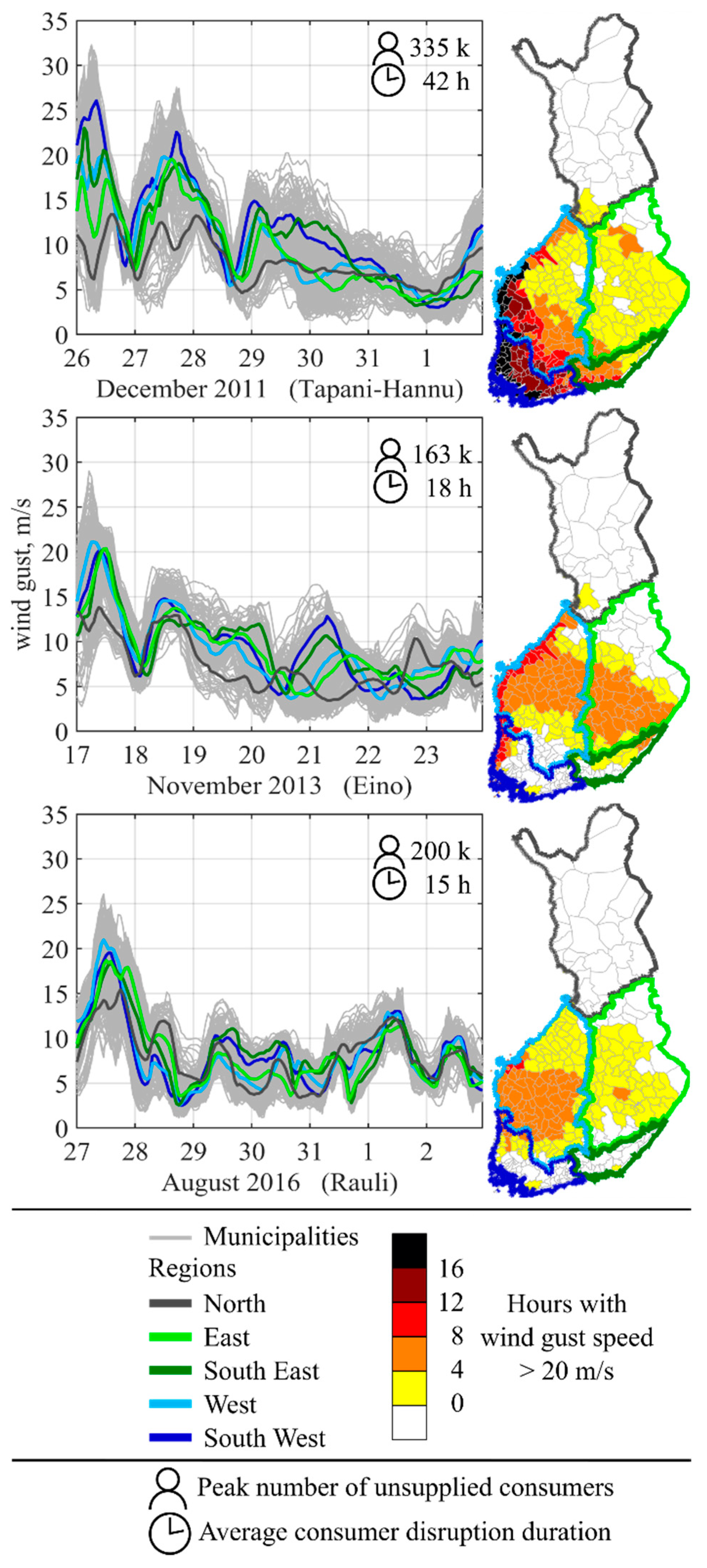
Rauli (27 August 2016) was the most damaging among the recent windstorms [46], despite its moderate wind gust speeds compared to the previously mentioned windstorms. Rauli is an excellent example of an impactful summer windstorm where factors other than the wind gust speed influenced the final damages. The impacts of Rauli were significant because of the time of the year: at the end of a rainy August, the soil was wet and unfrozen, and the trees had the maximum canopy cover, including leaves on the deciduous trees. In addition, summer windstorms are typically shorter in duration, and cover smaller areas (see Figure 2). However, Rauli was relatively long-lasting [51].

The wind gust fields for the weeks when the three selected windstorms occurred are shown in Figure 2. Within these fields, only the values above 15 m/s matter; 15 m/s is an assumed limit, above which repair work can no longer take place, while fault probabilities become significant at approximately 18 m/s. In Finland, the volume of forest damage during windstorms has been observed to follow the wind gust speed, as a function of wind gust speed with a power of ten [24]. Given that falling trees are the main powerline fault mechanism, it should not be surprising that there is also an indication of a power relation between the wind gust speed and faults [34]. Thus, the aggregated representation of wind hazard can be difficult. Nonetheless, aggregations using a statistical moment (e.g., the regional averages in the Figure 2 temporal profiles) or duration above a certain threshold (e.g., as done for the Figure 2 spatial profiles) correlate, and give similar distributions. The figure also includes the peak number of consumers without power, and the average interruption duration for each windstorm case. The values are derived from the dataset containing individual faults, compiled by the consultancy company Enease [52,53]. This dataset is presented in detail in the next section. The dataset does not contain information about repeating faults, which prohibits the derivation of the total number of customers affected that is commonly reported in secondary sources (Tapani–Hannu, 570 k [45,46], Eino, 230 k [2,46,49], Rauli, 200 k [46]). The average duration is computed as the ratio between the total consumer hours interrupted, and the peak number of consumers interrupted, which makes the average larger than it would be by computing the ratio with the total number of consumers interrupted. The interruption values for Rauli in the figure also account for scaling to match the secondary source, as explained in Section 4.1.

All the selected cases share some similarities, most notably the absence of soil frost, that are indicative of the model’s applicability. Soil frost is a well-known major impact-driving factor that is not accounted for in the model. Therefore, a model calibrated for one of these cases is unlikely to be suited for windstorms that occur during periods when soil frost is present. On the other hand, the most damaging windstorms that occur, and are expected to continue occurring, do so in the absence of soil frost. Additionally, long-term windiness trends show no indication that future windstorms will have significantly higher wind speeds. It is worth noting that there are some studies suggesting that the wind fields of the windstorms may get larger in the future, increasing the area exposed to strong winds, as well as causing a poleward shift in the storm tracks, possibly resulting in more windstorms in Finland [54,55]. However, taken together, most of the evidence seems to indicate the model’s ability to produce impact profiles for the most impactful future windstorms to be similar to its ability to recreate historic impact profiles.

3. Electricity System Resilience

Energy system resilience refers to the ability of the energy system to survive, and recover from, major disruptions, and is typically quantified by the system performance throughout all the phases of disruption [56]. Obtaining information on this performance requires modeling the energy system operation through the disruption, with an account of the potential faults and repairs. This section presents a summary of the framework for such modeling, and the information captured by it that can be used as an indicator of the resilience of the system.

3.1. Modeling Framework

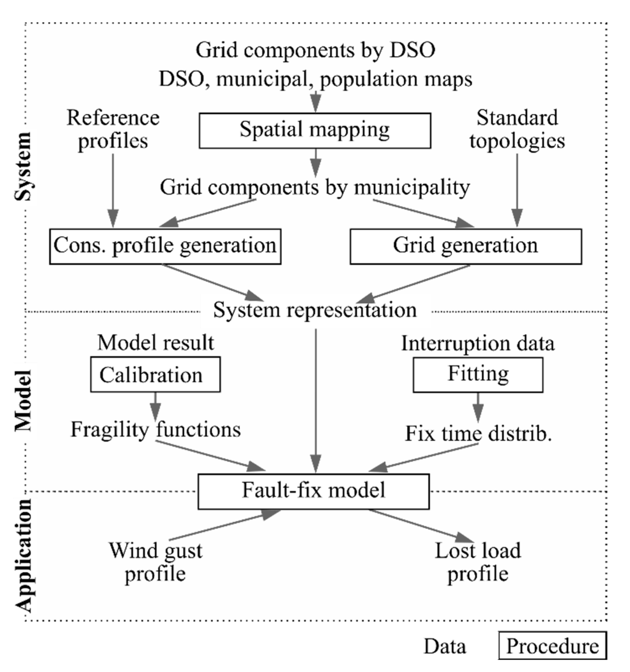
Figure 3 shows the structure of the modeling framework, documented in detail in [3], with three major parts. The first part generates a synthetic electricity grid and consumption profiles. The generated electricity grid covers the whole of Finland (except for the Åland islands), with MV granularity, where the basic segment is an MV line between the two MV to low voltage (LV) transformers. The system contains over 130 k of these segments (the exact number varies with the year of the study case). The consumption profiles distinguish the dependency on time (hourly resolution), space (municipal resolution), voltage level (medium and low), and consumer sectors (industrial, commercial, and residential). The second part combines the generated system with fragility functions and fixing-time distributions, both of which are derived from the historical power interruption data. The final part is the application of the model, by taking the spatiotemporal wind gust field of the case studies as an input, and giving the spatiotemporal LL profile as an output. The input data, along with their resolution, sources, and the part of the model in which they are used, are summarized in

Table 1. A summary of the model input data. LV/MV/HV stands for low/medium/high voltage, respectively. The interruption record contains data on the occurrence, duration, affected consumption, and number of consumers. In 2020, Finland had 309 municipalities, and interruption data are available for DSO service areas aggregated into five regions.

Variable	Resolution		Source		Used in
	Spatial	Temporal
Number of transformers (MV, HV)	DSO service area	Year	Energy Authority (regulator)	[57,58]	Spatial mapping
Length of powerlines (MV)
Cabling rate (MV)
Number of consumers (MV)
Consumption (LV, MV)
DSO service area shapefiles	DSO service area	Year	Adato Energy (consultancy)	[59]	Spatial mapping
Municipality shapefiles	Municipality	Year	National Land Survey	[60]	Spatial mapping
Population data shapefiles	1 km × 1 km	Year	Statistics Finland	[61]	Spatial mapping
Consumption by sector	Municipality	Year	Finnish Energy (industry association)	[62]	Spatial mapping
Reference consumption profiles	Country	Hour	Energy Authority (regulator)	[63]	Profile generation
Dwelling units by building type	Municipality	Year	Statistics Finland	[64]	Profile generation
Consumption	Country	Hour	Finnish Energy (industry association)	[65]	Profile generation
Temperature	31 km × 31 km	Hour	ERA5 reanalysis	[40,41]	Profile generation
Wind gust speed					Application
Forested area share	Municipality	Year	Finnish Environmental Institute	[66]	Application
Interruption	Aggregated region	Second	Enease (consultancy)	[52,53]	Model and application

. The annual data depend on the year, and the hourly data also on the time of year of the study case but, in all cases, the same data sources are used.

3.2. Electricity System Vulnerability

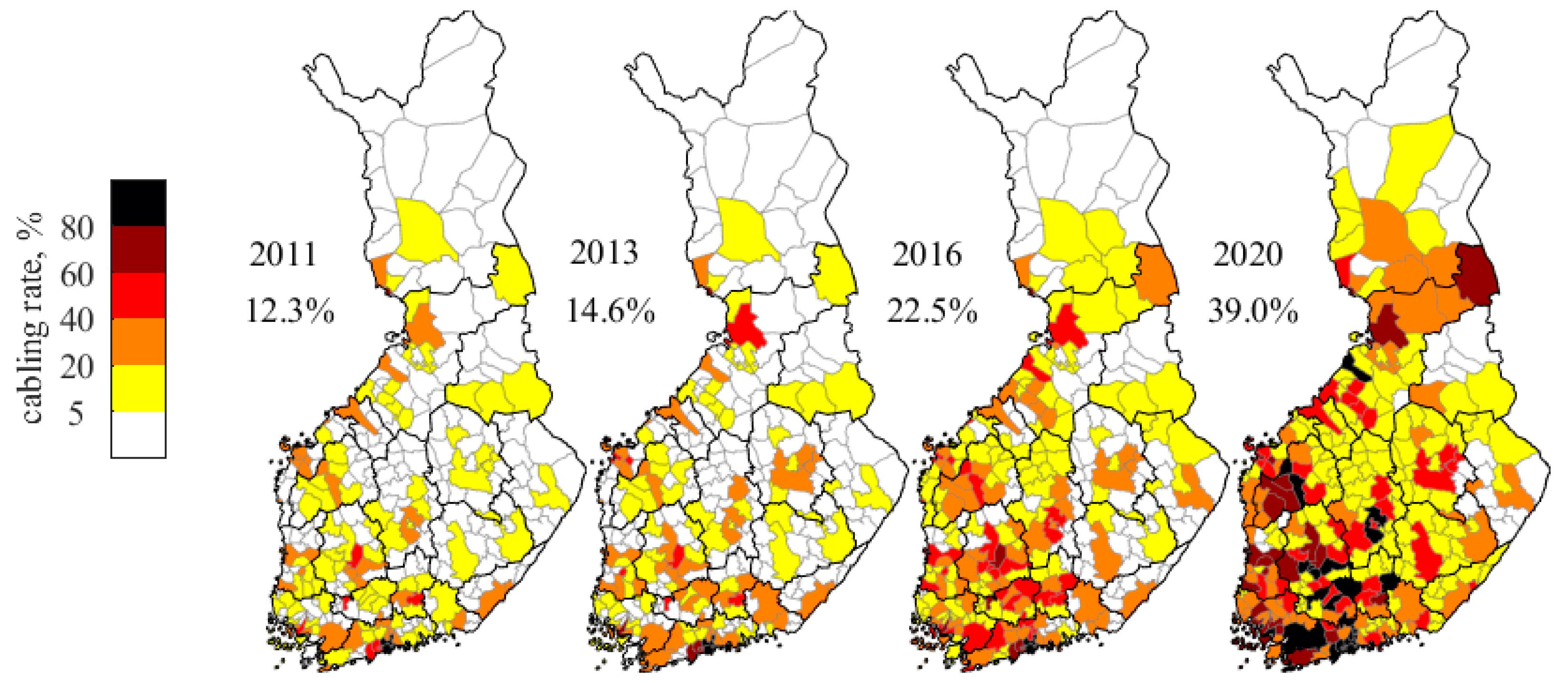
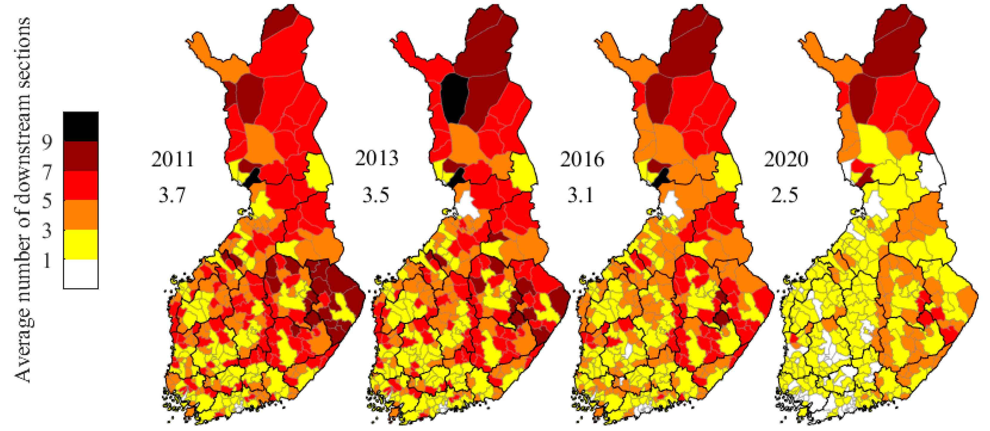
A good indication of electricity system vulnerability to wind hazard can be obtained from the electricity system representations (i.e., synthetic MV grids and consumption profiles) generated. Four such system representations were generated for the three years of the three windstorms introduced in Section 2.3, and for the year 2020, representing the current system. The most important change in Finnish electricity system vulnerability that has accrued during the 2011–2020 period was the underground cabling of powerlines, shown in Figure 4. Lines cabled underground are also typically placed along roadsides [67], which further reduces their vulnerability to windstorms, and the associated uprooting of trees. The level of cabled line vulnerability is illustrated by a negligible component of disruption costs, in the assessment of the powerline segment’s lifetime costs [67]. As a result, the powerlines cabled underground can be viewed as being mostly immune to windstorms, and are treated as such in the model. Furthermore, the cabling share can be used as an indicator of the share of the consumption at MV and LV levels that are no longer vulnerable to wind hazard. At the same time, the cabling carried out in the order of decreasing segment importance allows for a reduction in the average number of downstream nodes (see Figure 5) proportionally reducing the average impact of an individual fault. Regarding the consumption, there are no significant differences between years, while the seasonal consumption differences between the study-case-specific times of the year are accounted for during the generation of synthetic consumption profiles. The profile generation algorithm includes scaling up hourly reference profiles for the sector and municipality specific annual consumption totals, then normalizing the sum of the scaled profiles to match the national hourly consumption profile. Customer-type-specific reference profiles are provided by the Finnish energy system regulator at an hourly resolution for the whole year of 2018. The day-type selection used to map the reference consumption profiles from the weeks in 2018 to the weeks in the case studies is presented in Supplementary Material Section S1.

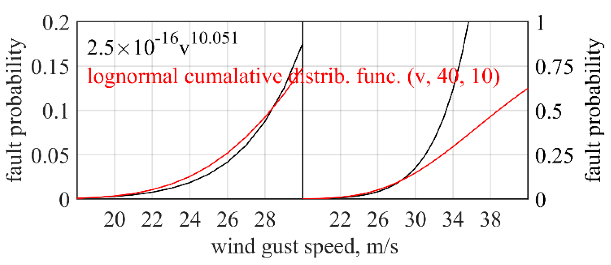
Another major indicator of electricity system resilience is the fragility of its components, described by fragility functions. The fragility functions in all four systems were kept the same, as no solid basis was found to detect changes for them throughout the years. Nevertheless, the form for the fragility functions was changed for this work. The original fragility function in [3] had a power function form which, with the higher wind speeds than studied before, lead to fault probabilities over one. To enable the model’s application for more severe wind gust speed ranges, the new function form was changed to lognormal. The lognormal function form enables an account of larger wind gust speeds, without resulting in unrealistic probabilities over one. The lognormal form is also a commonly used form for modeling mechanical engineering phenomena in general [14], and the fragility functions of electricity system components in particular [17,68]. The parameters for the lognormal function (expected value of 40, and standard deviation of 10) were chosen in such a way that the fragility functions in both forms were similar in the wind gust speed range between 18 m/s and 30 m/s, as shown in Figure 6. The wind gust speed of 18 m/s is when faults start to occur, and 30 m/s is close to the record of the windstorm for which the original function was fitted. The range of 18–30 m/s is close to the 16–27 m/s reported to represent the range dominated by faults occurring from a complex set of factors [69]. Modeling this complexity with fragility functions is difficult, resulting in the predictions of machine-learning-based models being more accurate [69]. However, above this range, all the fault mechanisms become dominated by wind, and thus a single physics-based fragility function form is well suited to represent the dependency [69]. The parameters of the original power-form fragility function were obtained by calibrating the modeled LL profile for the largest windstorm in Finnish grid history [3]. Calibration refers to running the model multiple times, with different fragility functions, and selecting one function with which the LL profile is the closest to the recorded reference profile. No additional calibrations were made here for the LL profiles from other historical windstorms.

3.3. Interruption Data Analysis

The account of interruption data is a significant factor for impact modeling ability, as it is used to derive the fragility functions, and the fix-time distributions. This is especially true in cases when the model is used for historically unprecedented windstorms, as the modeling results are sensitive to any extrapolation of derived relationships. The aim to capture as much information from the interruption data as possible includes the use of all available data, their analysis at the maximum justifiable detail, and the scrutiny of their reliability.

The interruption data used here include a list of individual faults, with information on the fault cause, time, and duration, the number of disrupted consumers, and their annual consumption. These data are collected by the former energy consultancy company Enease Ltd. (Helsinki, Finland), and were obtained for research purposes in aggregated form for five large areas in Finland, to anonymize company-specific data [52,53]. Data were collected and combined from individual DSOs from 2005 until 2019, and used for yearly power outage statistics reports [70]. Since 2019, Finnish Energy has no longer collected data from the individual DSOs, and does not produce the yearly power outage statistics, due to the lack of staff resources. Thus, the data analyzed in this paper cover the years 2005–2018 and include 235 k entries of faults caused by the wind.

The smallest subsets of these entries that can be analyzed independently are arguably the storm and calm periods, as they represent independent meteorological events. Such a grouping is performed here using only the interruption data, i.e., without meteorological data. A storm period was chosen as a set of sequential days with over 100 faults for at least one hour. An hourly NoFs was computed by summing the duration portions of all faults that at least in part fell within that hour. For example, if the fault occurred at 0:30 and lasted until 1:00 or later, its contribution to the NoFs in the first hour of the day would be 0.5. Windstorms, and the dominant share of the associated generation of new faults, typically last a few hours, and can extend up to a day. However, a large NoFs after a major windstorm can take multiple days to clear. In other words, the storm periods discussed in this paper represent the periods of windstorm impact on the grid, rather than periods of strong wind. A calm period is chosen as constituting a year quarter with all non-storm days, a period with a relatively limited change in the grid and environment conditions. The faults were grouped, with the storm and calm periods, by the day that the fault started, regardless of the fault duration.

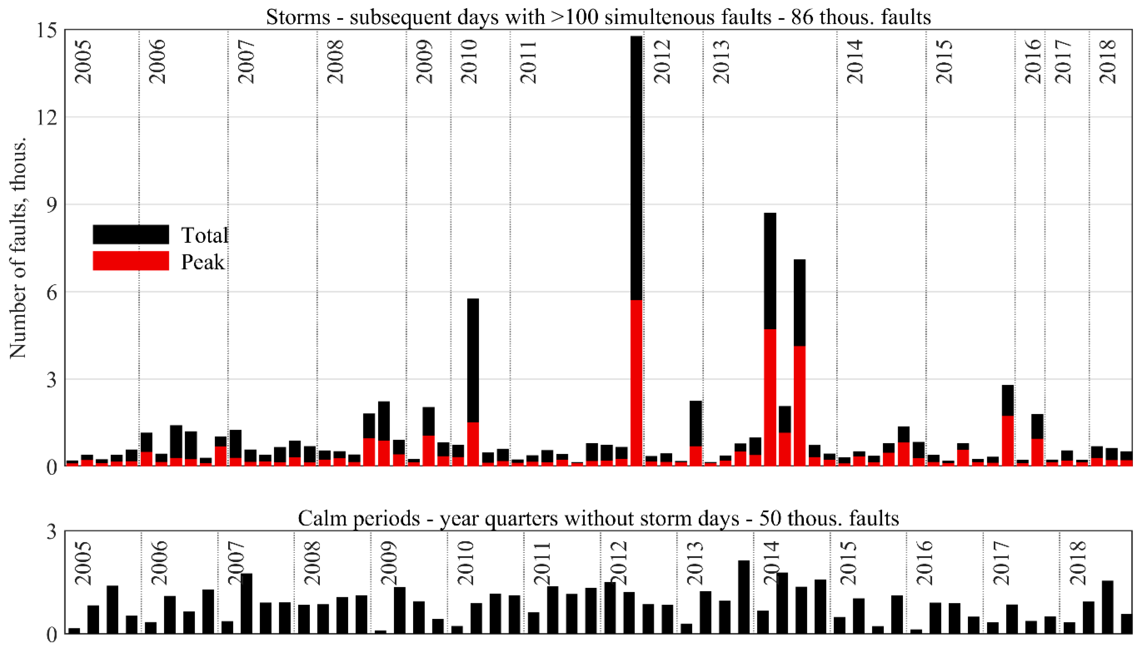
The fault duration distributions of each storm and calm period were discretized for the comparison of these periods, and for the derivation of the severity-dependent fix-time distribution that is discussed in the next subsection. The discretization was performed by taking the NoFs in a duration interval between the neighboring hour integers as a sum of all durations within that interval, divided by the upper integer. For example, if there were 100 faults with durations from 1 to 2 h that added up to a total of 160 h, it would be represented as 80 2 h long faults in a discretized distribution. This procedure conserved the fault hours and lost load, while reducing the total number of entries in the distribution, predominantly among the short faults. A significant portion of the power interruptions in the analyzed dataset had durations of a few minutes or less. These interruptions were most likely resolved via automatic means, without the dispatch of physical repair crews, and thus are not a primary concern of the current modeling work. Nevertheless, it is expected that the reduced weight with discretization would be a superior approximation to the complete removal of faults shorter than some arbitrarily selected duration level. An overview of the resulting total and peak NoFs for the storm and calm periods is shown in Figure 7. Figure 7 highlights the significance of the few largest windstorms that occurred rarely and irregularly.

The analysis of the interruption data quality indicates that the data from 2015 onwards, which include 29 k wind fault entries, are of questionable reliability. In 2015, data collection practices changed, to increase the data granularity [71], but the direct impact of this change is not known. Observations made from the data quality analysis that raise concerns about newer data reliability include a significantly higher share of entries with internally inconsistent or implausible data; a lower share of faults caused by the wind, and a higher share from unknown sources; distinct clustering in storm-specific statistics (the fix-time distributions and averages of LL per fault); and a major mismatch with the secondary source for the LL profile of the selected windstorm. The statistics of the interruption data reliability, and the profiles from the secondary sources on which these observations were made, are presented in Supplementary Material Sections S2 and S3. The distinct clustering of the storm fix-time distributions is presented in the next subsection. Due to reliability concerns, the post-2014 fault data are not used for fitting the fix-time distributions, while for the construction of LL reference profiles, they are used only in combination with the secondary data.

3.4. Fixing Times

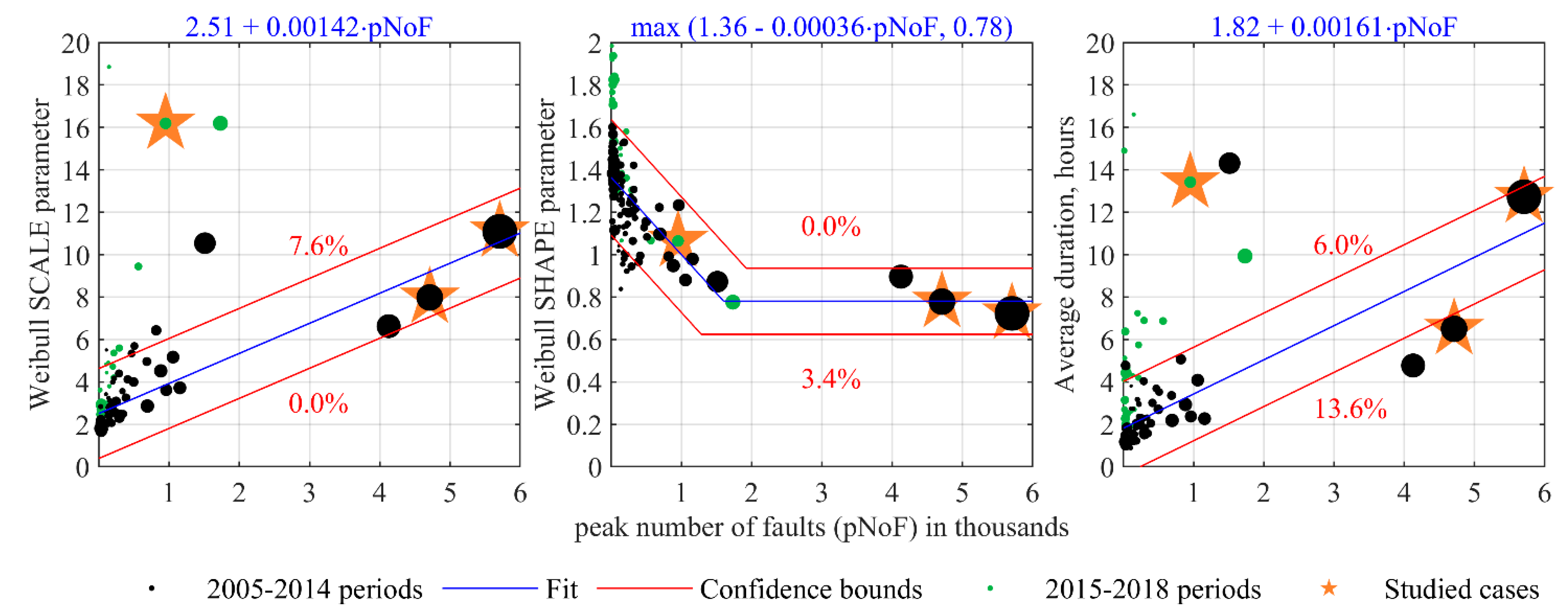
The fixing times are modeled with the storm severity-dependent distribution, to account for repair queues in the presence of a limited repair capacity. As in [3], the severity-dependent distribution is generated through the fitting of the discretized fault-duration distributions of fault subsets with the Weibull distribution, and then the fitting of the obtained Weibull parameters for their dependency on the peak NoFs. However, here, the generation is performed using 2005–2014 fault entries, grouped into 98 storm and calm periods that differ 150 times in the total NoFs, instead of the 2011–2012 fault entries grouped into three comparable size categories. This changes the methodological rationale, the required calculation step details, and the subsequent results.

The rationale of a methodology with essentially two fitting levels can be justified by the fact that the fits on the first level are carried out for the distributions resulting from independent meteorological events. At the same time, a large number of storm and calm periods provides many points for the second level fit. In turn, this provides a strong statistical basis for the reliability of the generated severity-dependent distribution. This also allows the capturing of the variability between the different periods, indicating the level of uncertainties present. On the other hand, some periods include relatively few entries, complicating their fit to the Weibull distribution. To avoid occasional bad fits, a floor of 77% for the goodness of fit was imposed, by rejecting the fit, and repeating the procedure of fitting, until a satisfactory fit was obtained. To account for the wide variation in the number of elements between periods, the second-level fit was performed with the total NoFs as the period weights.

The resulting first-level fits and their quality are shown in Supplementary Material Section S4, while the second-level fits are shown in Figure 8. The second-level fits were selected to be of the simplest linear form. However, the linear extrapolation of the shape parameter dependency can lead to negative values, which are outside of the Weibull distribution parameter bounds. To avoid such unrealistic outcomes, three storm periods with the largest peak NoFs were excluded from the shape-parameter fitting, and a floor for the minimum value was enforced. The minimum value chosen was equal to the shape parameter of the storm period with the second-largest peak NoFs.

Figure 8 includes several additional elements to aid the interpretation of results. Firstly, the rightmost panel of the plot shows the linear dependency fitted for the average duration. The average duration is not used in the latter analysis, but is easy to interpret, and largely corresponds to the scale parameter of the Weibull distribution. Secondly, the green dots show the values for the post-2014 data, assumed less reliable, and thus excluded from the fitting procedure. They show distinct clustering toward longer interruptions, compared to the rest of the data. Thirdly, the confidence bounds and share of faults outside these bounds indicate the fit representativeness. The confidence bounds are set equal to 20% of the largest parameter value, within the historic range of peak NoFs. Stricter confidence bounds, equal to 20% of the fitted value, are set for the shape parameter in the range, with an imposed floor value. The 20% level is based on the indication of the model accuracy in recreating the LL profiles for historic windstorm cases (see Section 4.2). Alternatively, confidence bounds could be derived directly from the interruption data, using mathematical methods such as the Kolmogorov–Smirnov test. However, it is not obvious whether such a mathematical procedure would represent the actual level of uncertainty, given the multitude of technical and environmental factors that differ between windstorms, and affect repair times. Moreover, the small shares of faults beyond the 20% bounds indicate the high representativeness of these bounds. Fourthly, the figure highlights the parameters for the historic windstorm cases studied individually in the next section.

4. Replicating Historic Impacts

Replicating the impact profiles for historic windstorms is arguably the most important test for the model, as there are no direct ways to test the model validity for studies beyond the historic record. The model is applied to three windstorm cases, selected according to their impact severity and recentness, as described in Section 2.3. The recreation of the LL profiles is the primary objective for the model, as the cost from load interruptions can be significantly higher than the direct cost of the physical damage to the electricity grid. Nevertheless, the number of failed segments aids in the analysis of the study cases, and thus is also included.

4.1. Means for Result Evaluation

The model results are compared to the LL and NoFs reference distributions in time, for the whole of Finland, and in space, with the distinction of five outage regions.

Hourly reference profiles for each outage region are derived primarily from the dataset of individual power interruptions described in Section 3.3. The profiles for the NoFs are directly constructed from this interruption dataset, by treating each entry as a fault, and applying the hourly discretization described previously in the same subsection. The construction of the LL profiles combines the data on the annual consumption of consumers disrupted by individual faults, with the hourly national consumption profile for Finland [65]. The two datasets are combined, assuming a constant consumption share of interrupted consumers throughout the year. The obtained LL profiles for the Tapani–Hannu and Rauli cases are compared with secondary sources (see Supplementary Material Section S3), with a good fit for Tapani–Hannu, and a large mismatch for Rauli. Because of the mismatch with data from secondary source for Rauli [72], and other issues with post-2014 data presented in Section 3.3, the LL profile is constructed by scaling down each Rauli interruption by a factor of three in amplitude, and a factor of two in duration, to match the secondary source. Despite imposed scaling, the LL profile for Rauli still benefits from the use of interruption data for individual faults, as they give information about the spatial distribution.

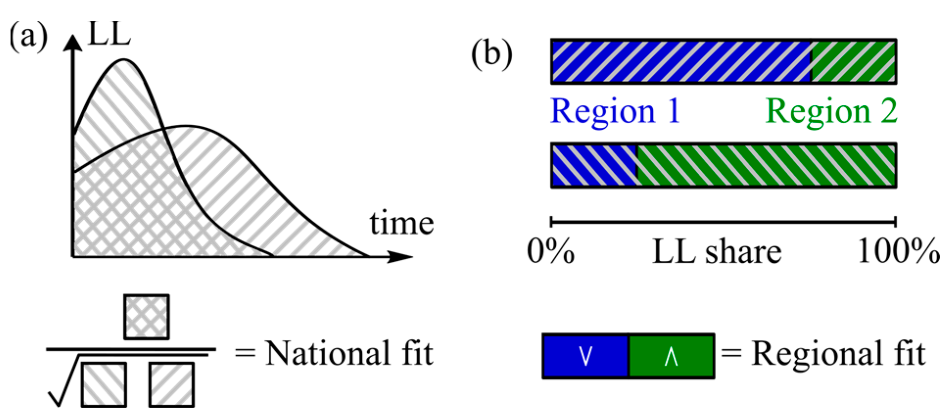
To quantify the model fit in recreating the reference profiles, two indicators are chosen. The first indicator shows the national fit equal to the ratio of overlapping area, and the geometric mean of the areas of the temporal profiles for the whole country (as indicated in Figure 9a) for the LL. This national fit indicator provides an intuitive metric that represents the ratio of visually observable areas. The national fit becomes the exact ratio of the areas when both profiles cover areas of the same size, which should not be far from the actual case, when the fit is relatively good. The mathematical expression of the national fit is:

$$National fit=\frac{{\mathrm{L}\mathrm{L}}_{mod}\cap {\mathrm{L}\mathrm{L}}_{ref}}{\sqrt{{\mathrm{L}\mathrm{L}}_{mod}·{\mathrm{L}\mathrm{L}}_{ref}}},$$

(1)

where $\mathrm{L}\mathrm{L}=$ lost load, $mod=$ model, and $ref=$ reference. The LL values are integrated over the time of the study period. The overlapping area is computed by integrating the minimum LL of the two profiles.

The second indicator shows the regional (i.e., spatial distribution) fit equal to the sum of regional shares that are smaller between the two profiles for the whole study period. This is illustrated for the case of two regions in Figure 9b, with the regional fit being equal to the sum of the lower profile share for region 1, and the upper profile share for region 2. The mathematical expression of regional fit is:

$$Regional fit={\sum }_{reg}^5\min \left({\left(\frac{\mathrm{L}{\mathrm{L}}_{reg}}{\mathrm{L}\mathrm{L}}\right)}_{mod},{\left(\frac{{\mathrm{L}\mathrm{L}}_{reg}}{\mathrm{L}\mathrm{L}}\right)}_{ref}\right),$$

(2)

where $reg=$ outage region. Again, the LL values in the equation are integrated over the time of the study period. Note that while the indicators in Figure 9 and Equations (1) and (2) are given for the LL, they apply identically for the NoFs.

The overlapping shares represent the intuitive quantification of the fit between two profiles, and are independent of the study period duration, as long as the profiles are captured. This quantification approach treats each fault hour and kWh of the LL equally. The cost of kWh may differ within the disruption profile, if the dependencies on the time of the day and the absolute disruption magnitude are accounted for, but such dependencies are outside the scope of the current work.

4.2. Model Results vs. Reference Profiles

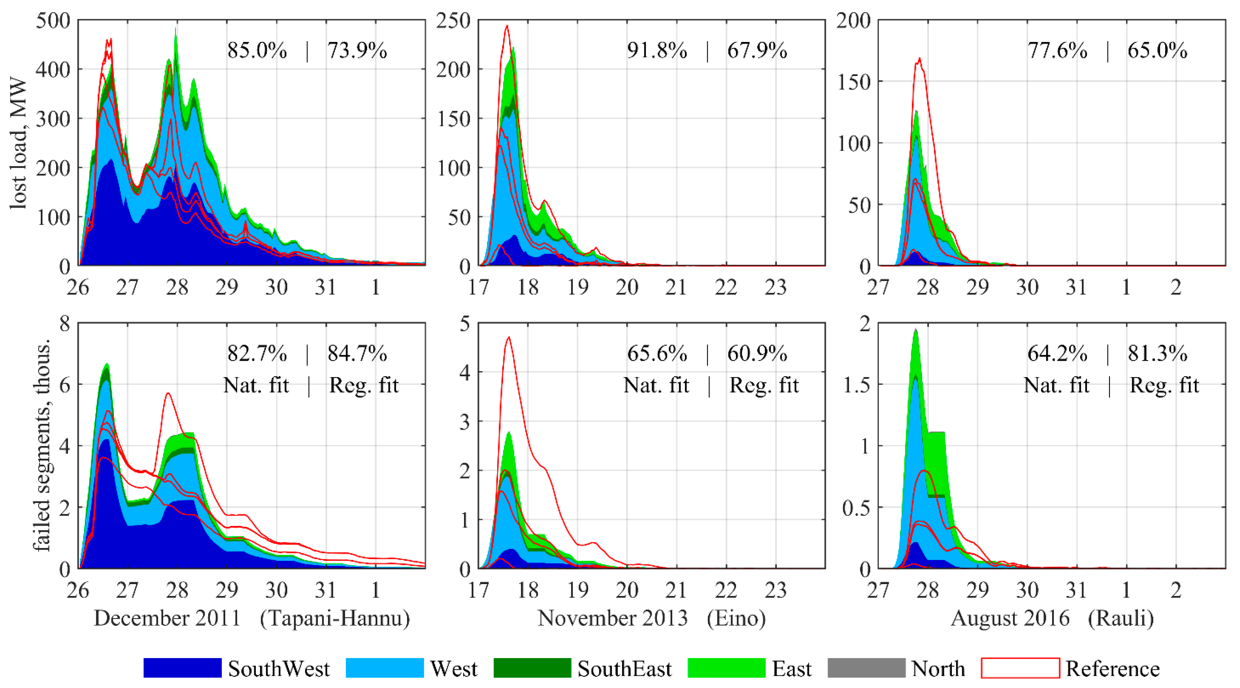
The model results in recreating the LL and NoFs profiles for historic windstorm cases are shown in Figure 10. The best fit values are for the national LL profiles, the replication of which is the primary objective of the model. These values are within a range of 77–92%, which gives a rough indication of uncertainties in the order of 20%.

Such a level of accuracy seems to be relatively good, considering the modeling approach, accuracy of other models, available data, and intended model use. The fragility-based modeling approach used here excludes a multitude of impact-driving factors with unknown significance. The accuracy comparison with other impact models is a complicated exercise in itself, but even data-intensive machine-learning-based models that account for hundreds of environmental variables retain non-insignificant uncertainties [8]. The available interruption data include only a few large windstorm cases, limiting the statistical basis for derived fragility functions, and severity-dependent fixing times. At the same time, the three studied windstorm cases contain 29% of the NoFs among all the storm periods in 2005–2018. Finally, the focus for the intended use of the model is on strategic energy system development and regulation questions, where the national impact scale may be of higher importance than the regional distribution.

The biggest mismatches between the model and reference profiles include the Rauli case, the underestimation of the disruption share in the east, and a worse match for the NoFs in all cases. The lower fit for the Rauli case is not surprising, given the more distinct windstorm (relatively low wind speeds and the presence of tree canopy) and primary data reliability concerns. The underestimation of impacts in the east indicates some regional differences that are not accounted for in the model. Examples of such factors could include looser soil, or trees that have adapted to grow in less windy conditions. Improving the regional fit requires a separate study of potentially relevant factors and, if found significant, their account in the model. The worse match for the NoFs is likely to be due to some differences between the distribution grid representation in the model and the real system that affect the NoFs without affecting the LL. One such difference could be the omission of disconnectors, due to the available data limitations, and the significant model complexity increase required. Disconnectors are devices that isolate damaged segments from the rest of the grid. Faults in the model are isolated within the MV line segment between two MV-to-LV transformers. This corresponds with the assumption that each MV-to-LV transformer has a disconnector, which is not the case in reality. The uneven distribution of disconnectors could be the cause of the higher NoFs mismatch while the associate error for the LL remains lower, as each fault disconnects the supply for a larger piece of the system. We should remember that a typical fault disconnects multiple segments downstream in a radial distribution grid (as shown in Figure 5). Whether this, or some other aspect, is the reason behind the larger NoFs mismatch, the expected remedy involves a more detail account of the distribution grid. However, the NoFs is considered a secondary variable for the target application, and thus not a priority for a major model expansion.

The modeled LL profile in the Tapani–Hannu case shows a good height fit for both the Tapani and Hannu peaks, but a good width fit only for the first Tapani peak. The height fit indicates the fit of the fragility function, as it primarily determines the upward part of the impact profile. A good height fit here shows that the form change for the fragility function was adequate, and there was neither a need for, nor a significant fit improvement potential from, recalibration. The width fit indicates the fit of the generated fixing-time distribution, as it primarily determines the downward part of the impact profile. It is worth recalling that the fitted dependency of the fix-time distribution parameters on the NoFs in Figure 8 resulted in a deviation from historic windstorm cases; i.e., the blue lines in Figure 8 did not go through the points describing the historic Tapani–Hannu distribution. Using historic distribution parameters may improve the fit for the modeled impact profile, but would defeat the purpose of the modeling, and is not possible for other (past or future) windstorm cases without historic impact data. Furthermore, a change in the severity-dependent fix-time distribution in the model would affect the downward profiles for both peaks. Thus, the improvement of the width fit for the Hannu peak would come at the price of the width fit for the Tapani peak. This suggests that the current representation of fix times only partially captures the repair work dynamics throughout two major windstorms separated by a period that does not allow for a full recovery from the first windstorm. However, this observation cannot be tested, due to the absence of another such pair of windstorms in Finland. On the other hand, the rarity of the Tapani–Hannu-like pair also suggests a low likelihood of encountering the associated underestimation of the second peak width in future windstorms. Alternatively, analytical methods for modeling fixing times may allow to avoid such problems. However, fixing times depend on the availability and position of repair personnel and material that depend on existing regulations and practices of grid operators [73]. Modeling such factors analytically would require a lot of difficult-to-obtain data and complex model formulations. Overall, even with underestimated width of the second peak, modeled LL profile for Tapani–Hannu matches the reference profile relatively well. Whether the model can generate similarly realistic impact profiles for other windstorms requires testing for other windstorms for which fragility functions were not calibrated.

The Eino and Rauli interruption data are not used for fragility function calibration in any form, but the results are similar to the Tapani–Hannu case. The national fit for the Eino windstorm is even better than that of Tapani–Hannu, capturing well both the height and the width of the impact profile. This indicates the model’s ability to produce realistic LL profiles for a range of windstorms, irrespective of the ways in which the Tapani and Hannu windstorms could be distinct. The national fit for Rauli is worse, but still relatively good, considering the significant differences in the natural environment, most notably the presence of tree leaves. The period between Tapani–Hannu and Rauli also covered significant changes in the electricity system, including an underground cabling rate growth from 12% to 39%, as well as other grid-hardening measures not accounted for in the model. Therefore, the fit for the Rauli profile further indicates the model’s ability to produce relatively realistic impact profiles for a range of windstorms that include significant differences.

5. Conclusions

This work presents an exploration of the ability of the fragility-based impact model with a detailed electricity system representation to generate realistic LL profiles for the most impactful windstorm cases, along three lines of evidence. The conclusions for each explored line of evidence are the following.

Wind impact:

• The impacts of windstorms on the electricity system are driven by a multitude of region-specific environmental, infrastructural, and organizational factors.
• The account of the significance of these factors, let alone the representation in a fragility-based impact model, is difficult.
• Attempts to quantify these factors have been few, especially in the Finnish environment.
• Most impactful windstorms share some similarities, which are expected to remain present in the most impactful future windstorms.

Grid resilience:

• Grid-cabling efforts in the last decade have significantly reduced Finnish electricity grid vulnerability to wind hazards.
• Storm and calm periods provide an optimal grouping basis for interruption data analysis, as they can be considered to present individual meteorological events.
• The two-level fitting of fixing times with such grouping provides a strong statistical basis for the resulting severity-dependent distribution and indication of the associated uncertainties (around 20%) that are difficult to capture through analytical means.
• The fragility functions and fixing-time distributions are designed to be applicable beyond the historical windstorm severity range, even though there are no direct means to validate the model ability there.

Impact modeling:

• A fragility-based model accounting for only a few factors can reproduce major windstorm impact profiles for different windstorm and grid cases, without recalibration.
• The collective evidence indicates that the presented model can generate realistic national LL profiles for the most impactful windstorms in Finland, with uncertainties in the order of 20%.
• The obtained level of accuracy is expected to be sufficient for the intended model use in studies on strategic electricity system development, and broader emergency preparedness questions.

The exploration of the model’s ability was limited to high-severity windstorms occurring in the absence of soil frost, and the absence of coinciding with other major hazards to powerlines, such as a heavy snow load on trees. Further investigation is needed to determine if the model is applicable to cases outside of the mentioned limits, potentially with the recalibration of the fragility functions. For windstorm cases where the model is applicable, the most notable limitations appear to be a lower accuracy for the number of faults (compared to LL) and for spatial distribution (compared to the national temporal profile). On the other hand, the model’s reliance on the interruption data and statistical methods of deriving severity-dependent fixing-time distributions does not seem to be of significant concern.

The presented modeling framework is expected to be applicable to other highly forested countries at the mid-latitudes, as no unique aspects for Finland were encountered during the study. Therefore, the exploration performed, in addition to providing strong evidence of the presented model’s applicability in Finland, also provides indirect evidence of a similar model’s ability in other countries. The indirect evidence is of high value, given the rarity of major windstorms. This also means that similar studies in other countries would provide relevant evidence of the fragility-based model’s use in Finland.

The feasibility of analogous exploration studies in other countries would depend on the availability of interruption data, and the data needed to construct an impact model with detailed electricity system representation. The former is arguably more crucial, as there are multiple ways to generate synthetic grids and consumption profiles based on proxy data. That said, exploration should be tailored to account for country-specific impact-driving factors and their evolution. This includes both grid (i.e., dominant hardening measures) and natural environment (i.e., vegetation and climate) factors. In Finland, a major change on the grid side was the underground cabling, and on the weather side, a major variable that could change in the future is the presence and depth of soil frost. In other countries, however, the most relevant changes among impact-driving factors are likely to be different.

Considering future work, running additional historic cases would be beneficial, but the added value would be less than the value obtained from the study of the initial set of cases. The following planned work is the application of the model to a historically unprecedented but meteorologically plausible windstorm case in Finland, to provide a basis for the exploration of cost-driving factors in higher-severity disruptions. Alternative directions for future work that are also promising include runs with longer study periods, more rigorous treatment of uncertainties, extending the analytical representation of the model to faults and repairs that currently rely on historic interruption statistics, and testing the model on other types of storm with grid-damaging winds, and on storms in different environmental conditions.

References

1. Bompard, E.; Huang, T.; Wu, Y.; Cremenescu, M. Classification and Trend Analysis of Threats Origins to the Security of Power Systems. Int. J. Electr. Power Energy Syst. 2013, 50, 50–64. [Google Scholar] [CrossRef]
2. Gregow, H.; Laurila, T.K.; Mäkelä, A.; Rantanen, M. Review on Winds, Extratropical Cyclones and Their Impacts in Northern Europe and Finland; Finnish Meteorological Institute: Helsinki, Finland, 2020.
3. Jasiūnas, J.; Heikkinen, T.; Lund, P.D.; Láng-Ritter, I. Resilience of Electric Grid to Extreme Wind: Considering Local Details at National Scale. Reliab. Eng. Syst. Saf. 2023, 232, 109070. [Google Scholar] [CrossRef]
4. Forssén, K. Resilience of Finnish Electricity Distribution Networks against Extreme Weather Conditions. Master’s Thesis, Aalto University, Espoo, Finland, 2016. [Google Scholar]
5. Nurmi, V.; Pilli-Sihvola, K.; Gregow, H.; Perrels, A. Overadaptation to Climate Change? The Case of the 2013 Finnish Electricity Market Act. EconDisCliCha 2019, 3, 161–190. [Google Scholar] [CrossRef] [Green Version]
6. Tervo, R.; Láng, I.; Jung, A.; Mäkelä, A. Predicting Power Outages Caused by Extratropical Storms. Nat. Hazards Earth Syst. Sci. 2021, 21, 607–627. [Google Scholar] [CrossRef]
7. McRoberts, D.B.; Quiring, S.M.; Guikema, S.D. Improving Hurricane Power Outage Prediction Models Through the Inclusion of Local Environmental Factors. Risk Anal. 2018, 38, 2722–2737. [Google Scholar] [CrossRef]
8. Watson, P.L.; Spaulding, A.; Koukoula, M.; Anagnostou, E. Improved Quantitative Prediction of Power Outages Caused by Extreme Weather Events. Weather Clim. Extrem. 2022, 37, 100487. [Google Scholar] [CrossRef]
9. Nateghi, R.; Guikema, S.; Quiring, S.M. Power Outage Estimation for Tropical Cyclones: Improved Accuracy with Simpler Models. Risk Anal. 2014, 34, 1069–1078. [Google Scholar] [CrossRef]
10. Popović, Ž.N.; Kovački, N.V.; Popović, D.S. Resilient Distribution Network Planning under the Severe Windstorms Using a Risk-Based Approach. Reliab. Eng. Syst. Saf. 2020, 204, 107114. [Google Scholar] [CrossRef]
11. Xue, J.; Mohammadi, F.; Li, X.; Sahraei-Ardakani, M.; Ou, G.; Pu, Z. Impact of Transmission Tower-Line Interaction to the Bulk Power System during Hurricane. Reliab. Eng. Syst. Saf. 2020, 203, 107079. [Google Scholar] [CrossRef]
12. Zhai, C.; Chen, T.Y.; White, A.G.; Guikema, S.D. Power Outage Prediction for Natural Hazards Using Synthetic Power Distribution Systems. Reliab. Eng. Syst. Saf. 2021, 208, 107348. [Google Scholar] [CrossRef]
13. Prettico, G.; Gangale, F.; Mengolini, A.; Lucas, A.; Fulli, G. Distribution System Operators Observatory: From European Electricity Distribution Systems to Reference Network; EU JRC Institute for Energy and Transport: Luxembourg, 2016. [Google Scholar]
14. Panteli, M.; Pickering, C.; Wilkinson, S.; Dawson, R.; Mancarella, P. Power System Resilience to Extreme Weather: Fragility Modeling, Probabilistic Impact Assessment, and Adaptation Measures. IEEE Trans. Power Syst. 2017, 32, 3747–3757. [Google Scholar] [CrossRef] [Green Version]
15. Clements, D.; Mancarella, P. Fragility Curve Based Storm Modelling of Distribution Networks with Staff Constraints. In Proceedings of the IET International Conference on Resilience of Transmission and Distribution Networks (RTDN 2017), Birmingham, UK, 26–28 September 2017; pp. 1–5. [Google Scholar]
16. Jamieson, M.R.; Strbac, G.; Bell, K.R.W. Quantification and Visualisation of Extreme Wind Effects on Transmission Network Outage Probability and Wind Generation Output. IET Smart Grid 2020, 3, 112–122. [Google Scholar] [CrossRef]
17. Scherb, A.; Garrè, L.; Straub, D. Evaluating Component Importance and Reliability of Power Transmission Networks Subject to Windstorms: Methodology and Application to the Nordic Grid. Reliab. Eng. Syst. Saf. 2019, 191, 106517. [Google Scholar] [CrossRef]
18. Fu, G.; Wilkinson, S.; Dawson, R.J.; Fowler, H.J.; Kilsby, C.; Panteli, M.; Mancarella, P. Integrated Approach to Assess the Resilience of Future Electricity Infrastructure Networks to Climate Hazards. IEEE Syst. J. 2018, 12, 12. [Google Scholar] [CrossRef] [Green Version]
19. Mutanen, A. Improving Electricity Distribution System State Estimation with AMR-Based Load Profiles. Ph.D. Thesis, Tampere University of Technology, Tampere, Finland, 2018. [Google Scholar]
20. Perrels, A.; Haakana, J.; Hakala, O.; Kujala, S.; Láng-Ritter, I.; Lehtonen, H.; Lintunen, J.; Pohjola, J.; Sane, M.; Fronzek, S.; et al. Kustannusarviointi Ilmastonmuutokseen Liittyvästä Toimimattomuudesta (KUITTI) (Assessment of the Cost of Inaction Regarding Climate Change (KUITTI)); Publications of the Government’s Analysis, Assessment and Research Activities 2022:37; Valtioneuvoston Kanslia: Helsinki, Finland, 2022. [Google Scholar]
21. Ouyang, M.; Dueñas-Osorio, L. Multi-Dimensional Hurricane Resilience Assessment of Electric Power Systems. Struct. Saf. 2014, 48, 15–24. [Google Scholar] [CrossRef]
22. Räisänen, O.; Haapaniemi, J.; Haakana, J.; Lassila, J.; Partanen, J.; Ahonen, J.; Kurki, L. Assessing Overhead Line’s Susceptability to Storm Wind Damage Using Open Data. In Proceedings of the CIRED 2021—The 26th International Conference and Exhibition on Electricity Distribution, Online, 20–23 September 2021; Volume 2021, pp. 2794–2798. [Google Scholar]
23. Noebels, M.; Quirós-Tortós, J.; Panteli, M. Decision-Making Under Uncertainty on Preventive Actions Boosting Power Grid Resilience. IEEE Syst. J. 2022, 16, 2614–2625. [Google Scholar] [CrossRef]
24. Valta, H.; Lehtonen, I.; Laurila, T.K.; Venäläinen, A.; Laapas, M.; Gregow, H. Communicating the Amount of Windstorm Induced Forest Damage by the Maximum Wind Gust Speed in Finland. Adv. Sci. Res. 2019, 16, 31–37. [Google Scholar] [CrossRef] [Green Version]
25. Roberts, J.F.; Champion, A.J.; Dawkins, L.C.; Hodges, K.I.; Shaffrey, L.C.; Stephenson, D.B.; Stringer, M.A.; Thornton, H.E.; Youngman, B.D. The XWS Open Access Catalogue of Extreme European Windstorms from 1979 to 2012. Nat. Hazards Earth Syst. Sci. 2014, 14, 2487–2501. [Google Scholar] [CrossRef]
26. Gardiner, B.; Byrne, K.; Hale, S.; Kamimura, K.; Mitchell, S.J.; Peltola, H.; Ruel, J.-C. A Review of Mechanistic Modelling of Wind Damage Risk to Forests. For. Int. J. For. Res. 2008, 81, 447–463. [Google Scholar] [CrossRef] [Green Version]
27. Safety Investigation Authority. July-August 2010 Fierce Weather (Heinä-Elokuun 2010 Rajuilmat); Safety Investigation Authority: Helsinki, Finland, 2010. [Google Scholar]
28. Gregow, H.; Peltola, H.; Laapas, M.; Saku, S.; Venäläinen, A.; Laapas, H. Combined Occurrence of Wind, Snow Loading and Soil Frost with Implications for Risks to Forestry in Finland under the Current and Changing Climatic Conditions. Silva Fenn. 2011, 45, 35–54. [Google Scholar] [CrossRef] [Green Version]
29. Kilpeläinen, A.; Gregow, H.; Strandman, H.; Kellomäki, S.; Venäläinen, A.; Peltola, H. Impacts of Climate Change on the Risk of Snow-Induced Forest Damage in Finland. Clim. Chang. 2010, 99, 193–209. [Google Scholar] [CrossRef]
30. Venäläinen, A.; Tuomenvirta, H.; Heikinheimo, M.; Kellomäki, S.; Peltola, H.; Strandman, H.; Väisänen, H. Impact of Climate Change on Soil Frost under Snow Cover in a Forested Landscape. Clim. Res. 2001, 17, 63–72. [Google Scholar] [CrossRef] [Green Version]
31. Gardiner, B.; Blennow, K.; Carnus, J.-M.; Fleischer, P.; Ingemarson, F.; Landmann, G.; Lindner, M.; Marzano, M.; Nicoll, B.; Orazio, C.; et al. Destructive Storms in European Forests: Past and Forthcoming Impacts; European Forest Institute: Joensuu, Finland, 2010. [Google Scholar]
32. Gardiner, B. Wind Damage to Forests and Trees: A Review with an Emphasis on Planted and Managed Forests. J. For. Res. 2021, 26, 248–266. [Google Scholar] [CrossRef]
33. Liu, S.; Ji, X.; Zhang, X. Effects of Soil Properties and Tree Species on Root–Soil Anchorage Characteristics. Sustainability 2022, 14, 7770. [Google Scholar] [CrossRef]
34. Haakana, J.; Räisänen, O.; Karhunen, M.; Láng-Ritter, I. Impact of Wind Speed and Ground Frost on Electricity Distribution System Interruptions. Reliab. Eng. Syst. Saf. 2023, in press.
35. Laurila, T.K.; Gregow, H.; Cornér, J.; Sinclair, V.A. Characteristics of Extratropical Cyclones and Precursors to Windstorms in Northern Europe. Weather Clim. Dyn. 2021, 2, 1111–1130. [Google Scholar] [CrossRef]
36. Laurila, T.K. Winds and Windstorms in Northern Europe and Finland. Ph.D. Thesis, Ilmatieteen laitos-Finnish Meteorological Institute, Helsinki, Finland, 2022. [Google Scholar]
37. Rimali, A. Analysis of Frozen Ground in Finland: Affecting Environmental Factors, Trends in Northern Finland and Applicability of Satellite Data. Master’s Thesis, University of Oulu, Oulu, Finland, 2019. [Google Scholar]
38. Gregow, H. Impact of Strong Winds, Heavy Snow Loads and Soil Frost Conditions on the Risks to Forests in Northern Europe. Ph.D. Thesis, University of Eastern Finland, Joensuu, Finland, 2013. [Google Scholar]
39. Lehtonen, I.; Venäläinen, A.; Kämäräinen, M.; Asikainen, A.; Laitila, J.; Anttila, P.; Peltola, H. Projected Decrease in Wintertime Bearing Capacity on Different Forest and Soil Types in Finland under a Warming Climate. Hydrol. Earth Syst. Sci. 2019, 23, 1611–1631. [Google Scholar] [CrossRef] [Green Version]
40. Hersbach, H.; Bell, B.; Berrisford, P.; Hirahara, S.; Horányi, A.; Muñoz-Sabater, J.; Nicolas, J.; Peubey, C.; Radu, R.; Schepers, D.; et al. The ERA5 Global Reanalysis. Q. J. R. Meteorol. Soc. 2020, 146, 1999–2049. [Google Scholar] [CrossRef]
41. ERA5 Hourly Data on Single Levels from 1979 to Present. Available online: https://cds.climate.copernicus.eu/cdsapp#!/dataset/reanalysis-era5-single-levels?tab=form (accessed on 3 December 2021).
42. Jeppesen, J. Fact Sheet: Reanalysis. Available online: https://www.ecmwf.int/en/about/media-centre/focus/2020/fact-sheet-reanalysis (accessed on 28 December 2022).
43. Gryning, S.-E.; Floors, R. Investigating Predictability of Offshore Winds Using a Mesoscale Model Driven by Forecast and Reanalysis Data. Metz 2020, 29, 117–130. [Google Scholar] [CrossRef]
44. Finnish Meteorological Institute Merkittäviä Myrskyjä Suomessa-Significant Storms in Finland. Available online: https://www.ilmatieteenlaitos.fi/merkittavia-myrskyja-suomessa (accessed on 2 January 2023).
45. Kufeoglu, S.; Lehtonen, M. Cyclone Dagmar of 2011 and Its Impacts in Finland. In Proceedings of the IEEE PES Innovative Smart Grid Technologies, Europe, Istanbul, Turkey, 12–15 October 2014; pp. 1–6. [Google Scholar]
46. Krohns-Välimäki, H. Development of a Situation Awareness System for Disturbance Management of Electricity Networks. Ph.D. Thesis, Tampere University of Technology, Tampere, Finland, 2018. [Google Scholar]
47. Finnish Meteorological Institute. Monthly Climate Review. December 2011 (Ilmastokatsaus. Joulukku 2011); Finnish Meteorological Institute: Helsinki, Finland, 2011.
48. Storms over Scandinavia. Available online: https://www.eumetsat.int/storms-over-scandinavia (accessed on 22 December 2022).
49. Finnish Meteorological Institute. Monthly Climate Review. November 2013 (Ilmastokatsaus. Marraskuu 2013); Finnish Meteorological Institute: Helsinki, Finland, 2013.
50. Storm History Blog: 2013 Eino Ja Seija, Reima Ja Oskari, “Elviira”-Ukkosmyrsky (Thunderstorms). Available online: https://myrskyvaroitus.com/index.php/myrskytieto/myrskyhistoria/37-2013 (accessed on 22 December 2022).
51. Finnish Meteorological Institute. Monthly Climate Review. Rauli Rose to the Heavyweight of the Storms (Ilmastokatsaus. Rauli Nousi Myrskyjen Raskaaseen Sarjaan); Finnish Meteorological Institute: Helsinki, Finland, 2016.
52. Enease Oy. Interruptions 2005–2014 (Keskeytykset 2005–2014). Received via Personal Communication with Anssi Seppälä; Enease Oy: Helsinki, Finland, 2017. [Google Scholar]
53. Enease Oy. Interruptions 2015–2018 (Keskeytykset 2015–2018). Received via Personal Communication with Anssi Seppälä; Enease Oy: Helsinki, Filand, 2019. [Google Scholar]
54. Priestley, M.D.K.; Catto, J.L. Future Changes in the Extratropical Storm Tracks and Cyclone Intensity, Wind Speed, and Structure. Weather Clim. Dyn. 2022, 3, 337–360. [Google Scholar] [CrossRef]
55. Sinclair, V.A.; Rantanen, M.; Haapanala, P.; Räisänen, J.; Järvinen, H. The Characteristics and Structure of Extra-Tropical Cyclones in a Warmer Climate. Weather Clim. Dyn. 2020, 1, 1–25. [Google Scholar] [CrossRef] [Green Version]
56. Jasiūnas, J.; Lund, P.D.; Mikkola, J. Energy System Resilience—A Review. Renew. Sustain. Energy Rev. 2021, 150, 111476. [Google Scholar] [CrossRef]
57. Energy Authority. Technical Indicators for Electricity Network Operation 2005–2015 (Sähköverkkotoiminnan Tekniset Tunnusluvut 2005–2015), Received upon Personal Request from Energy Authority; Energy Authority: Helsinki, Finland, 2021. [Google Scholar]
58. Energy Authority Technical Indicators for Electricity Network Operation 2016–2020 (Sähköverkkotoiminnan Tekniset Tunnusluvut 2016–2020). Available online: https://energiavirasto.fi/verkkotoiminnan-julkaisut (accessed on 4 July 2022).
59. Adato Energia Oy. DSO Service Area Responsibility Map 2015 Shapefile (Vastuual). Received via Personal Communication with Risto Heliö; Adato Energia Oy: Helsinki, Finland, 2020. [Google Scholar]
60. National Land Survey of Finland File Service of Open Data. Available online: https://tiedostopalvelu.maanmittauslaitos.fi/tp/kartta?lang=en (accessed on 18 November 2021).
61. Statistics Finland Population Grid Data 1 km × 1 km. Available online: https://stat.fi/org/avoindata/paikkatietoaineistot/vaestoruutuaineisto_1km_en.html (accessed on 18 November 2021).
62. Finnish Energy Electricity Use by Municipality in 2007 to 2020 (Sähkönkäyttö Kunnittain 2007–2020). Available online: https://energia.fi/uutishuone/materiaalipankki/sahkonkaytto_kunnittain_2007-2020.html (accessed on 18 November 2021).
63. Energy Authority Load Profiles (Kuormitusprofiilit). Available online: https://energiavirasto.fi/hinnoittelun-valvonta (accessed on 3 December 2021).
64. Statistics Finland Household-Dwelling Units by Tenure Status, Type of Building, Number of Persons, 2005–2020. Available online: https://pxdata.stat.fi/PxWeb/pxweb/en/StatFin/StatFin__asas/statfin_asas_pxt_115y.px/ (accessed on 3 December 2021).
65. Finnish Energy Hourly Data on Electricity (Sähkön Tuntidata). Available online: https://energia.fi/uutishuone/materiaalipankki/sahkon_tuntidata.html (accessed on 27 July 2022).
66. Finnish Environment Institute Land cover by Municipality at the 2nd Classification Level (Maanpeite Kunnittain 2. Luokit-telutasolla). Available online: https://www.syke.fi/fi-FI/Avoin_tieto/Paikkatietoaineistot/Paikkatietoanalyysien_tuloksia(37720) (accessed on 8 December 2021).
67. Partanen, J.; Lassila, J.; Haakana, J. Regulation and Development of Electricity Distribution Network Business (Sähkönjakeluverkkoliiketoiminnan Sääntely ja Kehittäminen); Lappeenranta University of Technology: Lappeenranta, Finland, 2020. [Google Scholar]
68. Jufri, F.H.; Widiputra, V.; Jung, J. State-of-the-Art Review on Power Grid Resilience to Extreme Weather Events: Definitions, Frameworks, Quantitative Assessment Methodologies, and Enhancement Strategies. Appl. Energy 2019, 239, 1049–1065. [Google Scholar] [CrossRef]
69. Hughes, W.; Zhang, W.; Cerrai, D.; Bagtzoglou, A.; Wanik, D.; Anagnostou, E. A Hybrid Physics-Based and Data-Driven Model for Power Distribution System Infrastructure Hardening and Outage Simulation. Reliab. Eng. Syst. Saf. 2022, 225, 108628. [Google Scholar] [CrossRef]
70. Power Outage Statistics 2010–2019 (Keskeytystilasto). Available online: https://energia.fi/tilastot/sahkotilastot/keskeytystilasto (accessed on 10 January 2023).
71. Finnish Energy. Interruption Statistics 2015 (Keskeytystilasto 2015); Finnish Energy: Helsinki, Finland, 2016. [Google Scholar]
72. Storm History Blog: 2016 Salomo ja Rauli kesämyrskyt (Summer storms). Available online: https://myrskyvaroitus.com/index.php/myrskytieto/myrskyhistoria/156-2016-salomo-ja-rauli-kesaemyrskyt (accessed on 10 February 2023).
73. Dunn, S.; Wilkinson, S.; Alderson, D.; Fowler, H.; Galasso, C. Fragility Curves for Assessing the Resilience of Electricity Networks Constructed from an Extensive Fault Database. Nat. Hazards Rev. 2018, 19, 04017019. [Google Scholar] [CrossRef] [Green Version]
Figure 1. Number of days with a national mean of daily maxima of wind gusts above the 15–20 m/s thresholds.
Energies 16 05678 g001
Figure 2. The wind gust distribution in time (left side) and space (right side), with the subsequent electricity disruption indicators. Sources: wind gust data, ERA5 reanalysis; disruptions, Enease.
Energies 16 05678 g002
Figure 3. The structure of the modeling framework developed in [3]. The figure is reproduced from the source paper.
Energies 16 05678 g003
Figure 4. The municipal and national evolution of MV powerline cabling rates in Finland.
Energies 16 05678 g004
Figure 5. The municipal and national evolution of the average number of MV line segments downstream of overhead MV line segments.
Energies 16 05678 g005
Figure 6. The fragility functions for a 1 km long MV overhead powerline segment.
Energies 16 05678 g006
Figure 7. The number of faults for the storm and calm periods.
Energies 16 05678 g007
Figure 8. The dependencies of the key distribution parameters on the severity of the storm/calm period. The dot sizes are proportional to the period’s total number of faults. The percentages present a share of the total number of faults outside the confidence bounds among the 2005–2014 periods.
Energies 16 05678 g008
Figure 9. Schematic illustration of the indicators for (a) the national and (b) the regional fit between the modeled and reference profiles of the lost load.
Energies 16 05678 g009
Figure 10. The spatiotemporal disruption profiles for historic windstorm cases: modeled versus reference. The reference profile curves are in the same order as the modeled profile areas.
Energies 16 05678 g010