Power Measurement Using Adaptive Chirp Mode Decomposition for Electrical Vehicle Charging Load

Abstract

Due to nonlinear components in the charging piles of electric vehicles, harmonics and nonstationary signals in the electric vehicle charging load bring voltage and current distortion, seriously affecting the accuracy of the power-related calculation in nonsinusoidal environments. This paper proposed a new approach to calculate the active power and root mean square values from decomposed components using the adaptive chirp mode decomposition (ACMD) method on voltage and current. The advantage of the ACMD-based method is that it correctly provides the power-related quantities of harmonics or nonstationary components for the electric vehicle charging load. The performance of the proposed method was verified using synthetic signals and simulation tests. The experimental results presented better estimations for each quantity defined in IEEE Standard 1459-2010, compared with the discrete wavelet transform approach.

1. Introduction

With the enhancement of environmental protection awareness, electric vehicles have been widely used in many countries to alleviate global warming and energy crisis [1,2]. Typically, electric vehicles obtain electrical energy from the power grid through charging piles, especially direct current (DC) charging piles, whereas due to nonlinear components contained in the batteries of the electric vehicles and charging piles, the charging behavior of the electric vehicles, especially fast charging mode, brings a large number of harmonic and nonstationary signals, resulting in voltage and current distortion on the grid side of the charging piles, i.e., the voltage or current waveform is not standard sinusoidal [3]. The nonsinusoidal waveform would seriously affect the accuracy of electricity metering; thus, the research on the power calculation for electric vehicles makes sense for fair trade between users and power companies, as well as the generation, transmission, and operation of electricity.

For the power calculation under nonsinusoidal conditions, Budeanu [4] and Fryze [5] first proposed the definition of power quantities, commonly referred to as power theories, based on frequency-domain or time-domain analysis, respectively. After that, the definitions of various power components have been developed by many researchers [6,7,8,9,10,11]. Among these, IEEE Standard 1459-2010 [12], as one of the most prominent power theories, provides definitions mainly based on Fourier transform analysis. Although Fourier transform can provide the frequency information of analytical signals, it is only suitable to analyze the stationary and periodic signals due to the missing time-domain information. Commonly, harmonics, sudden changes, and nonstationary signals are generated during the charging processing of electric vehicles [13]. For Fourier transform, it is not possible to extract the time–frequency information of nonstationary signals; thus, it would bring large errors in power calculation.

To address the limitation of Fourier transform, wavelet-related transforms, as one of the most widely used time–frequency analyses, have been applied to power calculation in nonsinusoidal environments. Discrete wavelet transform (DWT) is first applied to calculate the root mean square (RMS) and power values by decomposing the given signals into constituent frequency sub-bands [14,15]. According to the definition of IEEE Standard 1459-2010 [12], the DWT was utilized to estimate the power components in a single system [14] and a three-phase system [16]. Further, for maintaining the temporal resolution of each decomposition level, stationary discrete wavelet transform (SDWT) without downsampling was used for the power calculation [17]. To achieve uniform frequency bandwidth for each sub-band, discrete wavelet packet transform (DWPT) [18] or stationary DWPT [19] was proposed for power calculation.

Although wavelet-related transforms can decompose the signals into frequency sub-bands through a filtering process, there is the issue of energy leakage [20], i.e., the content of decomposed frequency sub-bands does not correspond to individual harmonics or special nonstationary signal components. If the sub-bands are used for the power calculation of individual harmonic components or special nonstationary signal components, the results cause inconsistencies from the real power. This limitation of wavelet-related transforms is not present in adaptive chirp mode decomposition (ACMD). The ACMD extracts signal modes one by one with good adaptability and high time–frequency resolution, widely used in many fields [21,22,23,24]. However, the ACMD has not been applied for power calculation in the literature.

Thus, according to the definition of the IEEE Standard 1459-2010 [12], this paper presents an ACMD-based method to calculate power-related quantities of the charging load of the electric vehicles through the charging piles, since the electric vehicles connect to the power grid through the charging piles. Based on a time–frequency representation of the voltage and current using the ACMD method, the power-related quantities are calculated for the fundamental, harmonic, and nonstationary components, respectively. The proposed method is suitable for estimating harmonics or nonstationary components of voltage and current signals on the grid side of the charging piles, improving the representation of power-related quantities in nonstationary conditions.

2. Proposed Method

This section first presents the general mathematical mode of the voltage and current signals, according to the principle of the charging piles of electric vehicles. And then, the ACMD method is introduced to decompose the voltage and current signals into each component. Finally, decomposed components are utilized to estimate the corresponding active power and the RMS value of the voltage and current signals for the electric vehicle charging load.

2.1. General Mathematical Mode of Charging Voltage and Current

Due to the wide use of power electronic devices in the charging piles, the charging for the batteries of electric vehicles brings harmonic current and nonstationary signals to the power grid. The general structure of the charging piles is mainly composed of a rectifier circuit, a power converter, and an output filter circuit, as shown in Figure 1. Alternating current (AC) power is rectified to DC power through a three-phase bridge uncontrollable rectifier circuit and then provided for the DC/DC power converter to output the required DC of the electric vehicles. Finally, DC is filtered to charge the batteries of the electric vehicles.

More studies on the load characteristics of electric vehicles show that the voltage and current waveforms on the grid side of the charging piles, collected at charging stations [13,25], contain multiple harmonics and nonstationary signals. Typically, the current waveform mainly includes 6 h ± 1 order harmonics, and the amplitude of the harmonics gradually decreases with the increase in the harmonic order, which further can be confirmed in the simulation model in Section 3.2.

Generally, the voltage and current on the grid side of the charging piles can be respectively expressed as

$$\begin{array}{cc}\hfill & u\left(t\right)=u_b\left(t\right)+\sum _{h=1}{u}_h\left(t\right)+u_s\left(t\right)\hfill \\ \hfill & =\sqrt{2}{U}_{b}sin(\omega t+{\phi }_b)+\sum _{h=1}\sqrt{2}{U}_{h}sin((6h\pm 1)\omega t+{\phi }_h)+u_s\left(t\right)\hfill \end{array}$$

(1)

and

$$\begin{array}{cc}\hfill & i\left(t\right)=i_b\left(t\right)+\sum _{h=1}{i}_h\left(t\right)+i_s\left(t\right)\hfill \\ \hfill & =\sqrt{2}{I}_{b}sin(\omega t+{\varphi }_b)+\sum _{h=1}\sqrt{2}{I}_{h}sin((6h\pm 1)\omega t+{\varphi }_h)+i_s\left(t\right),\hfill \end{array}$$

(2)

where ($u_b$, $u_h$, $u_s$) denote the fundamental, harmonic, and nonstationary components of the voltage signal, respectively; ($i_b$, $i_h$, $i_s$) denote the fundamental, harmonic, and nonstationary ones of the current signal, respectively; $\omega$ is the fundamental frequency in radians; and (${\phi }_b$, ${\phi }_h$, ${\varphi }_b$, ${\varphi }_h$) are the initial phases of the fundamental voltage, the h-th harmonic voltage, the fundamental current, and the h-th harmonic current, respectively.

To accurately calculate the charging power of charging piles for the electric vehicles, the ACMD is firstly applied to decompose the fundamental, harmonic, and nonstationary components from $u\left(t\right)$ and $i\left(t\right)$ in our work, and then the power-related quantities are calculated according to IEEE Standard 1459-2010 [12].

2.2. ACMD-Based Power-Related Calculation

2.2.1. Adaptive Chirp Mode Decomposition (ACMD)

The ACMD, as a recursive mode decomposition technique, can adaptively extract signal components one by one using the matching pursuit method. For a nonstationary signal $x\left(t\right)$ with m components, it can be modeled as

$$x\left(t\right)=\sum _{i=1}^m{x}_i\left(t\right)=\sum _{i=1}^m{A}_i\left(t\right)cos\left(2\pi {\int }_0^t{f}_i\left(\tau \right)d\tau +{\phi }_i\right),$$

(3)

where $A_i\left(t\right)$, $f_i\left(t\right)$, and ${\phi }_i$ denote the instantaneous amplitude, instantaneous frequency, and the initial phase of the i-th component, respectively. Based on the technique of frequency demodulation, a demodulation frequency ${\tilde{f}}_i\left(t\right)$ is introduced, and then Equation (3) can be reformulated as

$$x\left(t\right)=\sum _{i=1}^m\left\{p_i\left(t\right)cos\left(2\pi {\int }_0^t{\tilde{f}}_i\left(\tau \right)d\tau \right)+q_i\left(t\right)sin\left(2\pi {\int }_0^t{\tilde{f}}_i\left(\tau \right)d\tau \right)\right\},$$

(4)

with

$$\begin{array}{c}\hfill p_i\left(t\right)=A_i\left(t\right)cos\left(2\pi {\int }_0^t(f_i\left(\tau \right)-{\tilde{f}}_i\left(\tau \right))d\tau +{\phi }_i\right)\\ \hfill q_i\left(t\right)=A_i\left(t\right)sin\left(2\pi {\int }_0^t(f_i\left(\tau \right)-{\tilde{f}}_i\left(\tau \right))d\tau +{\phi }_i\right),\end{array}$$

(5)

where $cos\left(2\pi {\int }_0^t{\tilde{f}}_i\left(\tau \right)d\tau \right)$ and $sin\left(2\pi {\int }_0^t{\tilde{f}}_i\left(\tau \right)d\tau \right)$ denote two demodulation operators, and $p_i\left(t\right)$ and $q_i\left(t\right)$ denote two demodulated signals with a phase difference of ${90}^{\circ }$. In particular, $p_i\left(t\right)$ and $q_i\left(t\right)$ become slowly varying baseband signals and have the narrowest bandwidth when ${\tilde{f}}_i\left(t\right)=f_i\left(t\right)$.

To extract the i-th signal component $x_i\left(t\right)$, the ACMD solve the minimization problem as follows

$$\begin{array}{cc}\hfill \underset{\left\{p_i\left(t\right)\right\},\left\{q_i\left(t\right)\right\},\left\{f_i\left(t\right)\right\}}{min}& \left\{\parallel p_i^{{}^{″}}{\left(t\right)\parallel }_2^2+\parallel q_i^{{}^{″}}{\left(t\right)\parallel }_2^2+\gamma {\parallel x\left(t\right)-x_i\left(t\right)\parallel }_2^2\right\},\hfill \\ \hfill \mathrm{s}.\mathrm{t}.x_i\left(t\right)& =p_i\left(t\right)cos\left(2\pi {\int }_0^t{\tilde{f}}_i\left(\tau \right)d\tau \right)+q_i\left(t\right)sin\left(2\pi {\int }_0^t{\tilde{f}}_i\left(\tau \right)d\tau \right)\hfill \end{array}$$

(6)

where ${\parallel ·\parallel }_2$ denotes $L_2$ norm, ${(·)}^{{}^{″}}$ denotes the second derivative, two terms $\parallel p_i^{{}^{″}}{\left(t\right)\parallel }_2^2$ and $\parallel q_i^{{}^{″}}{\left(t\right)\parallel }_2^2$ are used as smoothness constraints for measuring bandwidth of the signal, $\gamma >0$ is the penalty factor, and the last term $\parallel x\left(t\right)-x_i{\left(t\right)\parallel }_2^2$ denotes the residue energy after the currently estimated i-th component is eliminated.

To implement ACMD decomposition in a computer, the signal $x\left(t\right)$ is sampled at discrete time $t=t_0,...,t_{N-1}$, where N is the number of samples. And then, the objective function of (6) can be written in a discrete form

$$L(p_i,q_i,f_i)={∥\mathbf{D}{p}_i∥}_2^2+{∥\mathbf{D}{q}_i∥}_2^2+\gamma {∥x-(p_i{c}_i+q_i{s}_i)∥}_2^2,$$

(7)

where $\mathbf{D}$ is a second-order difference matrix, given by

$$\mathbf{D}={\left[\begin{array}{cccccc}1& -2& 1& \cdots & \cdots & 0\\ 0& 1& -2& 1& \cdots & 0\\ ⋮& \ddots & \ddots & \ddots & \ddots & ⋮\\ 0& \cdots & \cdots & -1& 2& -1\end{array}\right]}_{(N-2)\times N},$$

and

$$\begin{array}{c}\hfill c_i=\mathrm{diag}[cos\left({\theta }_i\left(t_0\right)\right),...,cos\left({\theta }_i\left(t_{N-1}\right)\right)]\\ \hfill s_i=\mathrm{diag}[sin\left({\theta }_i\left(t_0\right)\right),...,sin\left({\theta }_i\left(t_{N-1}\right)\right)],\end{array}$$

with ${\theta }_i\left(t\right)=2\pi {\int }_0^t{\tilde{f}}_i\left(\tau \right)d\tau$, where $diag[·]$ denotes the diagonal matrix.

To solve the optimization problem in (7), an iterative algorithm is used to alternately update the demodulated signals $p_i$, $q_i$, and the frequency $f_i$. For the m-th iteration, with the current frequency $f_i^{(m-1)}$, the solutions of $p_i$ and $q_i$ are updated by setting $\partial L(p_i,q_i,f_i)/\partial p_i=0$ and $\partial L(p_i,q_i,f_i)/\partial q_i=0$, given by

$$\begin{array}{cc}\hfill p_i^{\left(m\right)}& ={\left(\frac{1}{\gamma }{\mathbf{D}}^{\mathrm{T}}\mathbf{D}+{\left(c_i^{\left(m\right)}\right)}^{\mathrm{T}}{c}_i^{\left(m\right)}\right)}^{-1}{\left(c_i^{\left(m\right)}\right)}^{\mathrm{T}}x\hfill \\ \hfill q_i^{\left(m\right)}& ={\left(\frac{1}{\gamma }{\mathbf{D}}^{\mathrm{T}}\mathbf{D}+{\left(s_i^{\left(m\right)}\right)}^{\mathrm{T}}{s}_i^{\left(m\right)}\right)}^{-1}{\left(s_i^{\left(m\right)}\right)}^{\mathrm{T}}x,\hfill \end{array}$$

(8)

respectively, and then, the instantaneous frequency $f_i$ is updated by

$$f_i^{(m+1)}=f_i^{\left(m\right)}+{\left(\frac{2}{\beta }{\mathbf{D}}^{\mathrm{T}}\mathbf{D}+\mathbf{I}\right)}^{-1}\Delta {\tilde{f}}_i^{\left(m\right)},$$

(9)

with

$$\begin{array}{ccc}\hfill \Delta {\tilde{f}}_i^{\left(m\right)}\left(t\right)& =& \frac{1}{2\pi }\frac{d}{dt}\left({\tan }^{-1}\left(\frac{{\mathrm{p}}_{\mathrm{i}}^{\left(\mathrm{m}\right)}\left(\mathrm{t}\right)}{{\mathrm{q}}_{\mathrm{i}}^{\left(\mathrm{m}\right)}\left(\mathrm{t}\right)}\right)\right)\hfill \\ & =& \frac{q_i^{\left(m\right)}\left(t\right){\left(p_i^{\left(m\right)}\left(t\right)\right)}^{\prime }-p_i^{\left(m\right)}\left(t\right){\left(q_i^{\left(m\right)}\left(t\right)\right)}^{\prime }}{2\pi \left({\left(p_i^{\left(m\right)}\left(t\right)\right)}^2+{\left(q_i^{\left(m\right)}\left(t\right)\right)}^2\right)},\hfill \end{array}$$

(10)

where $\beta >0$ is a weighting factor, and ${(·)}^{{}^{\prime }}$ denotes the derivative.

Since the iterative algorithm requires the initial frequency $f_i^{\left(0\right)}$ in advance, synchroextracting transform (SET) [26] is adopted to estimate $f_i^{\left(0\right)}$ in this study. The SET, as a novel postprocessing strategy of short-time Fourier transform, has the advantage of better energy concentration to provide good instantaneous initial frequency for iteration. The iterative process continues until there is little difference in the extracted signal component $x_i$ in two adjacent iterations. After the signal component $x_i$ is extracted from the raw signal, the residual signal is obtained by removing $x_i$ from the raw signal, and then the iteration can be applied to the residual signal to extract the next signal component sequentially.

The above procedure is repeated for M times, and the components of signal $x\left(t\right)$ are finally obtained as

$$x\left(t\right)=\sum _{k=1}^M{x}_k\left(t\right)+R_s\left(t\right),$$

(11)

where $R_s\left(t\right)$ denotes the residual signal after M components are separated from the original signal. More details of the iteration algorithm can be found in [27].

When the ACMD method is applied to the voltage and current signals of charging piles, the corresponding fundamental component, harmonic components, and nonstationary components are separated from each other, and then, the decomposed components are used to implement the calculation of the active power, the RMS values of the voltage and current.

2.2.2. Power Calculation

According to IEEE Standard 1459-2010 [12], the active power (P), the RMS values of the voltage (U) and current (I) are calculated as

$$\begin{array}{cc}\hfill P& =\frac{1}{KT}{\int }_{t=t_0}^{t_0+KT}u\left(t\right)\times i\left(t\right)dt,\hfill \end{array}$$

(12)

$$\begin{array}{cc}\hfill U& =\sqrt{\frac{1}{KT}{\int }_{t=\tau }^{\tau +KT}{u}^2\left(t\right)dt},\hfill \end{array}$$

(13)

and

$$\begin{array}{cc}\hfill I& =\sqrt{\frac{1}{KT}{\int }_{t=\tau }^{\tau +KT}{i}^2\left(t\right)dt},\hfill \end{array}$$

(14)

respectively, where $\tau$ and $\tau +KT$ are the start time and end time of measurements, respectively, and $kT$ is an integer multiple of the power system fundamental period.

Using $u\left(t\right)$ in (1) and $i\left(t\right)$ in (2), the active power P in (12) is expressed as

$$P=P_{bb}+P_{bh}+P_{bs}+P_{hb}+P_{hh}+P_{hs}+P_{sb}+P_{sh}+P_{ss}$$

(15)

with

$$\begin{array}{cc}\hfill P_{bb}& =\frac{1}{KT}{\int }_{t=t_0}^{t_0+KT}{u}_b\left(t\right)i_b\left(t\right)dt,P_{hh}=\frac{1}{KT}\sum _{h=1}{\int }_{t=t_0}^{t_0+KT}{u}_h\left(t\right)i_h\left(t\right)dt\hfill \\ \hfill P_{ss}& =\frac{1}{KT}{\int }_{t=t_0}^{t_0+KT}{u}_s\left(t\right)i_s\left(t\right)dt,\hfill \\ \hfill P_{bh}& =\frac{1}{KT}\sum _{h=1}{\int }_{t=t_0}^{t_0+KT}{u}_b\left(t\right)i_h\left(t\right)dt,P_{hb}=\frac{1}{KT}\sum _{h=1}{\int }_{t=t_0}^{t_0+KT}{u}_h\left(t\right)i_b\left(t\right)dt,\hfill \\ \hfill P_{bs}& =\frac{1}{KT}{\int }_{t=t_0}^{t_0+KT}{u}_b\left(t\right)i_s\left(t\right)dt,P_{sb}=\frac{1}{KT}{\int }_{t=t_0}^{t_0+KT}{u}_s\left(t\right)i_b\left(t\right)dt,\hfill \\ \hfill P_{hs}& =\frac{1}{KT}\sum _{h=1}{\int }_{t=t_0}^{t_0+KT}{u}_h\left(t\right)i_s\left(t\right)dt,P_{sh}=\frac{1}{KT}\sum _{h=1}{\int }_{t=t_0}^{t_0+KT}{u}_s\left(t\right)i_h\left(t\right)dt,\hfill \end{array}$$

(16)

where $P_{bb}$, $P_{hh}$, and $P_{ss}$ are the fundamental, harmonic, and nonstationary active power, respectively; and $P_{bh}$, $P_{hb}$, $P_{bs}$, $P_{sb}$, $P_{hs}$, and $P_{sh}$ are the distortion active powers, generated by the different cross-combinations from the fundamental/harmonic/nonstationary voltage and the fundamental/harmonic/nonstationary current, respectively.

Since

$${\int }_0^{2\pi }sin\left(n\omega t\right)sin\left(m\omega t\right)dt=0$$

for $n\ne m$, we have $P_{bh}=P_{hb}=0$. And then, $P_{bs}\simeq 0$, $P_{sb}\simeq 0$, $P_{hs}\simeq 0$, and $P_{sh}\simeq 0$ can be considered in statistics, although there are minor errors. Thus, according to References [25,28], ($P_{bs}$, $P_{sb}$, $P_{hs}$, and $P_{sh}$) can be ignored, and then, the simplified calculation of the active power in (15) is given by

$$P=P_{bb}+P_{hh}+P_{ss},$$

(17)

i.e., the active power is the summation of the fundamental, harmonic, and nonstationary active power.

Accordingly, we calculate the RMS values of the voltage and current as

$$U=\sqrt{U_b^2+U_h^2+U_s^2},I=\sqrt{I_b^2+I_h^2+I_s^2},$$

(18)

where ($U_b$, $U_h$, and $U_s$) are the RMS values of the fundamental, harmonic, and nonstationary voltage, respectively, and ($I_b$, $I_h$, and $I_s$) are the RMS values of the fundamental, harmonic, and nonstationary current, respectively.

In practice, the analog voltage and current are first digitalized, and the continuous integration operation would be converted into the discrete ones. Thus, the active power ($P_{bb}$, $P_{hh}$, and $P_{ss}$) in (17) can be calculated as

$$P_{bb}=\frac{1}{N}\sum _{n=0}^{N-1}{u}_b\left(n\right)\times i_b\left(n\right),P_{hh}=\frac{1}{N}\sum _{h=1}\sum _{n=0}^{N-1}{u}_h\left(n\right)\times i_h\left(n\right),P_{ss}=\frac{1}{N}\sum _{n=0}^{N-1}{u}_s\left(n\right)\times i_s\left(n\right),$$

(19)

where ($u_{b,h,s}\left(n\right)$, $i_{b,h,s}\left(n\right)$) are the digitalized data of ($u_{b,h,s}\left(t\right)$, $i_{b,h,s}\left(t\right)$) at the n-th sampling index, respectively, and N is the integration interval. Accordingly, the RMS values of the voltage and current in (18) can be calculated as

$$\begin{array}{cc}\hfill U_b& =\sqrt{\frac{1}{N}\sum _{n=0}^{N-1}{u}_b^2\left(n\right)},I_b=\sqrt{\frac{1}{N}\sum _{n=0}^{N-1}{i}_b^2\left(n\right)},\hfill \\ \hfill U_h& =\sqrt{\frac{1}{N}\sum _{h=1}\sum _{n=0}^{N-1}{u}_h^2\left(n\right)},I_h=\sqrt{\frac{1}{N}\sum _{h=1}\sum _{n=0}^{N-1}{i}_h^2\left(n\right)},\hfill \\ \hfill U_s& =\sqrt{\frac{1}{N}\sum _{n=0}^{N-1}{u}_s^2\left(n\right)},I_s=\sqrt{\frac{1}{N}\sum _{n=0}^{N-1}{i}_s^2\left(n\right)},\hfill \end{array}$$

(20)

for the fundamental, harmonics, and nonstationary components, respectively.

3. Experiments and Results

In this section, we evaluate the proposed ACMD-based estimation of RMS values and active power using synthetic signals and simulation tests. In the following experiments, the key parameters $\gamma$ and $\beta$ of the ACMD method are set as $\gamma ={10}^{-6}$ and $\beta ={10}^{-9}$, respectively. The performance of the ACMD-based method is compared with the DWT-based method, since DWT is a time–frequency method widely used in signal analysis for power systems. The relative error of the estimated quantity is calculated as

$$Error=\frac{|Ref-Est|}{Ref},$$

(21)

where $Ref$ is the reference value, and $Est$ is the estimated value from the ACMD or DWT method.

3.1. Nonstationary Synthetic Signal

To demonstrate the performance of the ACMD method in signal decomposition and power-related estimation, three stationary waveforms, containing the fundamental and two harmonics, and one nonstationary component, are considered in synthetic signals of the voltage and current, expressed as

$$\begin{array}{cc}\hfill u\left(t\right)& =u_1\left(t\right)+u_2\left(t\right)+u_3\left(t\right)+u_4\left(t\right),\hfill \\ \hfill & =\sqrt{2}\left(220sin(2\pi \times 50t)+20sin(2\pi \times 250t+2\pi )+5sin(2\pi \times 350t+\pi )\right)\hfill \\ \hfill & +e^{-0.3t}cos\left(2\pi (450t+0.5\pi cos(2\pi \times 30t))\right)),\hfill \end{array}$$

(22)

$$\begin{array}{cc}i\left(t\right)\hfill & =i_1\left(t\right)+i_2\left(t\right)+i_3\left(t\right)+i_4\left(t\right),\hfill \\ \hfill & =\sqrt{2}\left(25sin(2\pi \times 50t)+10sin(2\pi \times 250t)+5sin(2\pi \times 350t)\right)\hfill \\ \hfill & +2e^{-0.3t}cos\left(2\pi (450t+0.5\pi cos(2\pi \times 30t))\right)),\hfill \end{array}$$

(23)

where the fundamental frequency is 50 Hz, the sampling frequency is 1500 Hz for discretizing $i\left(t\right)$ and $u\left(t\right)$, and the time interval of the synthetic signal is 0.5 s in this experiment.

To visually evaluate the decomposition performance of ACMD and DWT methods, we show the resultant synthetic current waveform and each component in Figure 2a as the ground-truth ones, based on (22). After the DWT with mother wavelet ‘db4’ and ACMD methods are used to decompose the current $i\left(t\right)$, the decomposed components and reconstructed signal are shown in Figure 2b,c. According to the principle of the DWT method, the fundamental component can be extracted from three-level DWT decomposition, and its frequency is within that of the highest-level approximation coefficients, i.e., ca3 in Figure 2b. From the decomposed results of the DWT method shown in Figure 2b, we observe that there is a component that does not already exist in (22) within [93.75, 187.5] Hz. In addition, the obtained components within [0, 93.75] Hz are not pure fundamental components as expected but mixed with the leakage components from other frequency ranges. Similar patterns exist in other frequency ranges, whereas the ACMD method obtains each component, more closely to the ground-truth ones, compared with the results from the DWT method.

The calculated quantities and relative errors (‰) of the fundamental, harmonics, and nonstationary components are shown in

Table 1. Comparisons of estimated quantities of ACMD-based and DWT-based methods for synthetic signal.

Quantity		Reference Values	ACMD		DWT
Symbols	Parameters	Analytical	Value	Error (‰)	Value	Error (‰)
U	Voltage RMS (V)	220.97	220.82	0.68	220.87	0.45
I	Current RMS (A)	27.39	27.38	0.36	27.38	0.36
P	Active power (W)	5625.86	5618.00	1.40	5602.85	4.09
$U_b$	Fundamental voltage RMS (V)	220.00	219.85	0.68	217.96	9.27
$I_b$	Fundamental current RMS (A)	25.00	24.98	0.80	24.80	8.00
$P_{bb}$	Fundamental active power (W)	5500.00	5492.78	1.31	5399.46	18.28
$U_h$	Harmonic voltage RMS (V)	20.62	20.59	1.45	35.13	703.68
$I_h$	Harmonic current RMS (A)	11.18	11.17	0.89	10.85	29.52
$P_{hh}$	Harmonic active power (W)	125.00	124.66	2.72	186.88	495.04
$U_s$	Nonstationary voltage RMS (V)	1.31	1.07	183.21	6.46	3931.29
$I_s$	Nonstationary current RMS (A)	0.66	0.53	196.96	4.14	5272.72
$P_{ss}$	Nonstationary active power (W)	0.86	0.57	337.21	16.52	18,209.30

, where the reference values are directly calculated from the analytic expressions in (22), agreeing with IEEE Standard 1459-2010. The estimated quantities for the three-type components are calculated from the decomposed results from the ACMD and DWT methods. The results in Table 1 show that the DWT-based method causes small estimations for the fundamental and large ones for harmonic, especially for nonstationary components, resulting in bringing large estimated errors for each component. The main reason is its leakage issue as mentioned above, whereas compared with the DWT-based method, the ACMD-based method brings quantities closer to the reference values with fewer estimation errors.

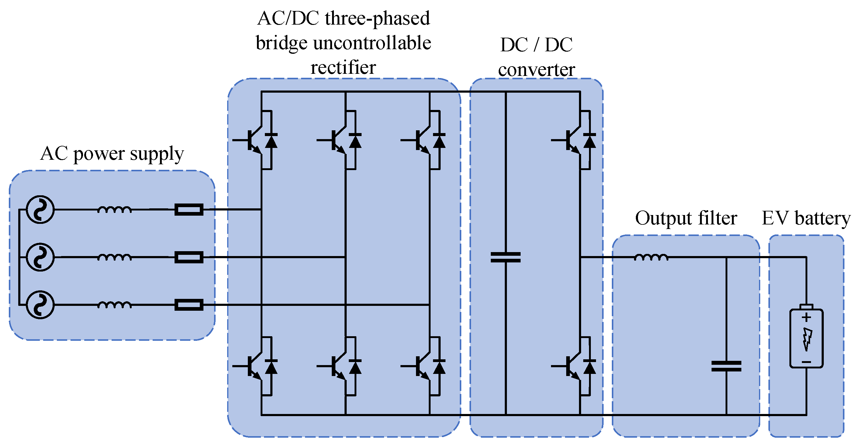
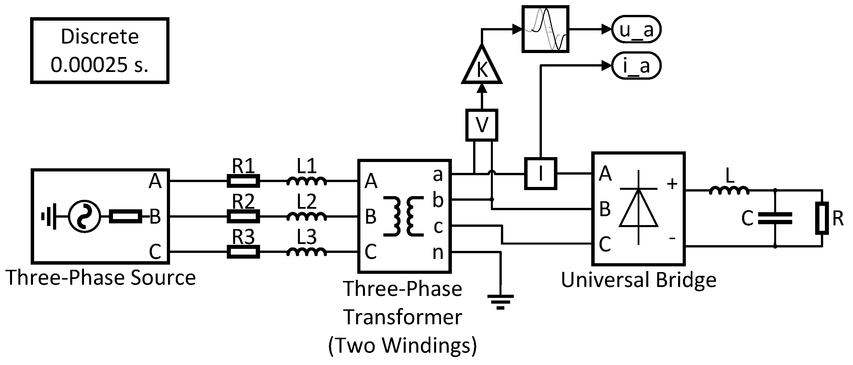
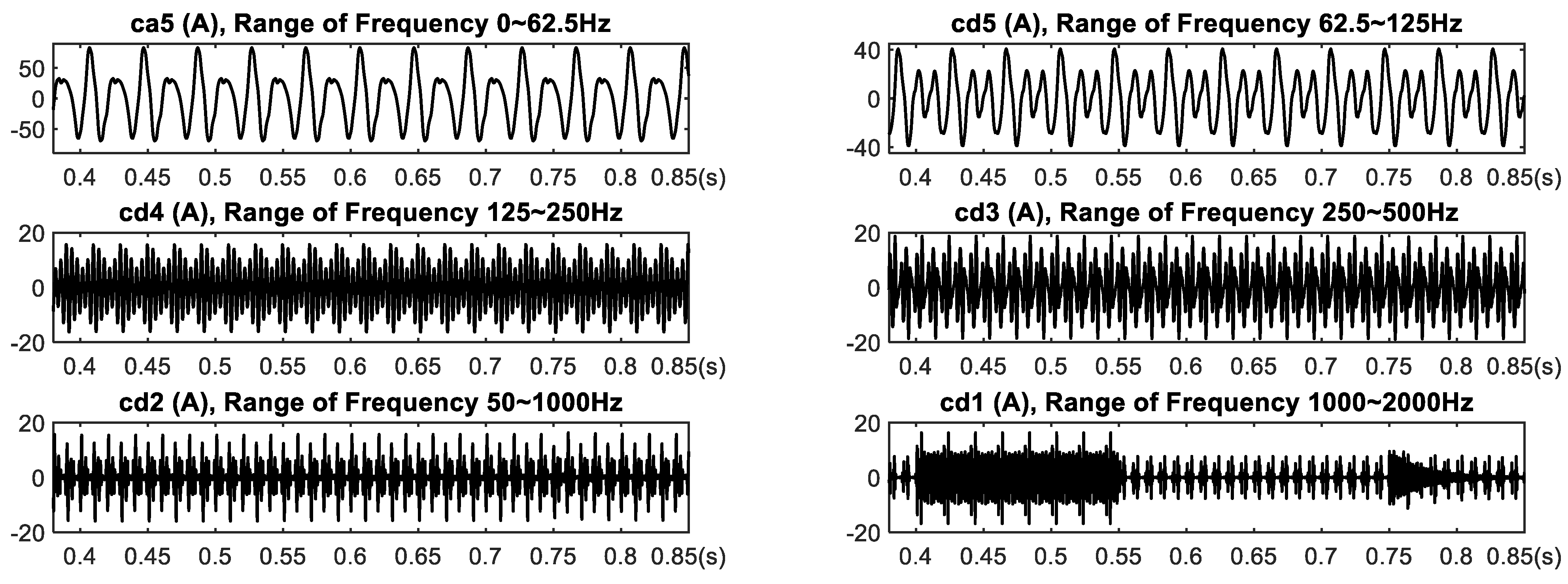
3.2. Simulation Signal

The performance of the proposed ACMD-based calculation method is further validated by using a simulation model in MATLAB/SIMULINK, as shown in Figure 3. The current and voltage waveforms at the grid side of the charging pile are shown in Figure 4a,b, respectively. From Figure 4, we observe that the charging current is similar to a square wave, deviating from the standard sine signal, while the voltage contains fewer harmonics, closer to the sine signal. Further, considering there are nonlinear elements in the charging piles of electric vehicles, the nonstationary signals are introduced to the current and voltage for realistically simulating the charging characteristics of electric vehicles. In this experiment, sawtooth impulse and high-frequency attenuation signals are used for the nonstationary signals $u_s$ and $i_s$, expressed as

$$u_s\left(t\right)=\left\{\begin{array}{cc}8\times sawtooth(2\pi \times 1800t+0.5\pi ,0.5),\hfill & t\in (0.4,0.55)s,\hfill \\ 8\times e^{-40t}sin(2\pi \times 1500t),\hfill & t\in (0.75,0.9)s,\hfill \end{array}\right.$$

(24)

and

$$i_s\left(t\right)=\left\{\begin{array}{cc}10\times sawtooth(2\pi \times 1800t+0.5\pi ,0.5),\hfill & t\in (0.4,0.55)s,\hfill \\ 10\times e^{-40t}sin(2\pi \times 1500t),\hfill & t\in (0.75,0.9)s,\hfill \end{array}\right.$$

(25)

respectively. Figure 4c shows the waveform of $i_s\left(t\right)$. To observe the components of current, the spectrum of the current $i\left(t\right)$ is shown in Figure 4d, which demonstrates that 6 h ± 1 order harmonics with successively attenuated amplitude appear on the corresponding spectral bins beside the fundamental, and the nonstationary signals appear on multiple high-frequency ranges, as shown in the enlarged drawing.

The sampling frequency is 4000 Hz in this experiment, and five-level DWT decomposition with the mother wavelet ‘db4’ is applied on current and voltage, making it that the highest-level frequency range corresponds to that of the fundamental component (i.e., ca5). Figure 5 shows the decomposed results of the current. From the decomposed fundamental and nonstationary components, it is easy to discern that both of them are mixed with other frequency components. Meanwhile, the ACMD method is utilized for current and voltage, and the decomposed results for the current are shown in Figure 6. Since the ACMD method performs decomposition recursively, two nonstationary signals are extracted separately, and close to the raw waveform in the views of waveform trend and occurrence interval. For harmonics, parts of the waveform within black windows are enlarged and displayed in small attached windows for comparison. Compared with the results from the DWT method in Figure 5, the decomposed components from the ACMD method in Figure 6 more agree with the real ones.

Using the decomposed components from the DWT and ACMD methods, the RMS values, active power, and relative error (‰) for the three components are calculated and shown in

Table 2. Comparisons of estimated quantities of ACMD-based and DWT-based methods for simulation signals in MATLAB/SIMULINK.

Quantity		Reference Values	ACMD		DWT
Symbols	Parameters	Analytical	Value	Error (‰)	Value	Error (‰)
U	Voltage RMS (V)	224.76	224.77	0.0	223.88	3.92
I	Current RMS (A)	49.54	49.62	1.61	49.49	1.01
P	Active power (W)	10,756.46	10,749.33	0.66	10,659.48	9.02
$U_b$	Fundamental voltage RMS (V)	224.41	224.46	0.22	200.07	108.46
$I_b$	Fundamental current RMS (A)	47.8200	47.83	0.21	42.74	106.23
$P_{bb}$	Fundamental active power (W)	10,686.11	10,691.48	0.50	8512.89	203.36
$U_h$	Harmonic voltage RMS (V)	10.49	10.75	24.78	100.39	8570.06
$I_h$	Harmonic current RMS (A)	12.60	12.74	11.11	24.69	959.52
$P_{hh}$	Harmonic active power (W)	48.48	51.07	53.42	2139.69	43,135.52
$U_s$	Nonstationary voltage RMS (V)	2.28	2.47	83.33	3.78	657.89
$I_s$	Nonstationary current RMS (A)	2.86	2.82	13.98	3.69	290.21
$P_{ss}$	Nonstationary active power (W)	6.54	5.79	114.48	6.89	53.45

. Since the real value for each component can not be calculated directly as the case for synthetic signals, the RMS values of the fundamental and harmonics are calculated from the corresponding information of spectral magnitude, while the quantities of the nonstationary component are calculated according to $u_s$ and $i_s\left(t\right)$ in (24) and (25). Similar to the comparison results for synthetic signals, the ACMD-based method achieves better estimation for each component and total active power for simulation data compared with the DWT-based method.

4. Conclusions

In this paper, a new approach based on the ACMD method was proposed to estimate the power-related quantities for electric vehicle charging load, according to the definition in the IEEE Standard 1459-2010 in the time–frequency domain. The current and voltage on the grid side of the charging piles were decomposed into the fundamental correctly, harmonic, and nonstationary components through the ACMD method. With the decomposed components, the active power and the RMS values were calculated for each component and the overall. Compared with the DWT-based method, the proposed ACMD-based method achieved better estimation of power-related quantities for the electric vehicle charging load with significantly fewer estimation errors, especially for the harmonics and nonstationary components. To further explore the advantage of the ACMD method for more applications in power systems, our future works will focus on power-related estimation of three-phase systems or other electric devices (e.g., power transformer) for abnormality detection, fault diagnosis, etc.

References

1. Zhao, H.; Wang, L.; Chen, Z.; He, X. Challenges of Fast Charging for Electric Vehicles and the Role of Red Phosphorous as Anode Material: Review. Energies 2019, 12, 3897. [Google Scholar] [CrossRef] [Green Version]
2. Liu, S.; He, K.; Pan, X.; Hu, Y. Review of Development Trend of Transportation Energy System and Energy Usages in China Considering Influences of Intelligent Technologies. Energies 2023, 16, 4142. [Google Scholar] [CrossRef]
3. Ding, X.; Shi, H.; Wang, Y.; Zhuang, Y.; Yuan, G.; Zhu, S. Research on Harmonic Management of Single-Phase AC Charging Pile Based on Active Filtering. Energies 2023, 16, 2817. [Google Scholar] [CrossRef]
4. Budeanu, C. Puissances Ractives et Fictives; Institut National Romain pour l’Étude de l’Aménagement et de l’Utilisation d’Énergie: Bucharest, Romania, 1927. [Google Scholar]
5. Fryze, S. Active, reactive and apparent power in circuts with nonsinusoidal voltages and currents. Przglad Elektro. 1931, 1, 193–203. [Google Scholar]
6. Miyasaka, G.; Silvério, E.; Xavier, G.; da Silva, H.; Braz, L.; Oliveira, R.; Lima, R.; Macedo, J. Analysis of Reactive Energy Measurement Methods Under Non-Sinusoidal Conditions. IEEE Lat. Am. Trans. 2018, 16, 2521–2529. [Google Scholar] [CrossRef]
7. Pajic, S.; Emanuel, A.E. Modern apparent power definitions: Theoretical versus practical Approach-the general case. IEEE Trans. Power Deliv. 2006, 21, 1787–1792. [Google Scholar] [CrossRef]
8. George, S.; Agarwal, V. A novel, DSP based algorithm for optimizing the harmonics and reactive power under non-sinusoidal supply voltage conditions. IEEE Trans. Power Deliv. 2005, 20, 2526–2534. [Google Scholar] [CrossRef]
9. De Almeida Coelho, R.; Brito, N.S.D. Power Measurement Using Stockwell Transform. IEEE Trans. Power Deliv. 2021, 36, 3091–3100. [Google Scholar] [CrossRef]
10. Morsi, W.G.; El-Hawary, M.E. Defining Power Components in Nonsinusoidal Unbalanced Polyphase Systems: The Issues. IEEE Trans. Power Deliv. 2007, 22, 2428–2438. [Google Scholar] [CrossRef]
11. Lev-Ari, H.; Stankovic, A.M. A decomposition of apparent power in polyphase unbalanced networks in nonsinusoidal operation. IEEE Trans. Power Syst. 2006, 21, 438–440. [Google Scholar] [CrossRef]
12. IEEE Std 1459-2010 (Revision of IEEE Std 1459-2000); IEEE Standard Definitions for the Measurement of Electric Power Quantities under Sinusoidal, Nonsinusoidal, Balanced, or Unbalanced Conditions. IEEE: New York, NY, USA, 2010; pp. 1–50.
13. Liu, J.; Xu, Q.; Tian, Z.; Guo, Y.; Qi, S.; Wang, L. Feature Extraction Method for DC Charging Signal of Electric Vehicle. In Proceedings of the 3rd Annual International Conference on Information System and Artificial Intelligence (ISAI2018), Hong Kong, China, 24–26 June 2016. [Google Scholar]
14. Morsi, W.G.; El-Hawary, M.E. Reformulating Power Components Definitions Contained in the IEEE Standard 1459-2000 Using Discrete Wavelet Transform. IEEE Trans. Power Deliv. 2007, 22, 1910–1916. [Google Scholar] [CrossRef]
15. Yoon, W.K.; Devaney, M. Reactive power measurement using the wavelet transform. IEEE Trans. Instrum. Meas. 2000, 49, 246–252. [Google Scholar] [CrossRef] [Green Version]
16. Morsi, W.G.; El-Hawary, M.E. Reformulating Three-Phase Power Components Definitions Contained in the IEEE Standard 1459-2000 Using Discrete Wavelet Transform. IEEE Trans. Power Deliv. 2007, 22, 1917–1925. [Google Scholar] [CrossRef]
17. Morsi, W.; El-Hawary, M. A new perspective for the IEEE standard 1459–2000 via stationary wavelet transform in the presence of nonstationary power quality disturbance. In Proceedings of the 2009 IEEE Power & Energy Society General Meeting, Calgary, AB, Canada, 26–30 July 2009; p. 1. [Google Scholar]
18. Osipov, D.S.; Dolgikh, N.N.; Goryunov, V.N.; Kovalenko, D.V. Algorithms of packet wavelet transform for power determination under nonsinusoidal modes. In Proceedings of the 2016 Dynamics of Systems, Mechanisms and Machines (Dynamics), Omsk, Russia, 15–17 November 2016; pp. 1–5. [Google Scholar]
19. Alves, D.K.; Costa, F.B.; de Araujo Ribeiro, R.L.; de Sousa Neto, C.M.; Rocha, T.D.O.A. Real-Time Power Measurement Using the Maximal Overlap Discrete Wavelet-Packet Transform. IEEE Trans. Instrum. Meas. 2017, 64, 3177–3187. [Google Scholar] [CrossRef]
20. Peng, Z.K.; Jackson, M.R.; Rongong, J.A.; Chu, F.L.; Parkin, R.M. On The Energy Leakage Of Discrete Wavelet Transform. Mech. Syst. Signal Process. 2009, 23, 330–343. [Google Scholar] [CrossRef] [Green Version]
21. Wang, X.; Tang, G.; Yan, X.; He, Y.; Zhang, X.; Zhang, C. Fault Diagnosis of Wind Turbine Bearing Based on Optimized Adaptive Chirp Mode Decomposition. IEEE Sens. J. 2021, 21, 13649–13666. [Google Scholar] [CrossRef]
22. Zhang, X.; Liu, Z.; Kong, Y.; Li, C. Mutual Interference Suppression Using Signal Separation and Adaptive Mode Decomposition in Noncontact Vital Sign Measurements. IEEE Trans. Instrum. Meas. 2022, 71, 1–15. [Google Scholar] [CrossRef]
23. Wang, H.; Chen, S.; Zhai, W. Data-driven adaptive chirp mode decomposition with application to machine fault diagnosis under non-stationary conditions. Mech. Syst. Signal Process. 2023, 188, 109997. [Google Scholar] [CrossRef]
24. Ding, C.; Wang, B. Sparsity-assisted adaptive chirp mode decomposition and its application in rub-impact fault detection. Measurement 2022, 188, 110539. [Google Scholar] [CrossRef]
25. Qi, S.R. Research on the Influence of Electrical Vehicle Charging Load on Electric Energy Measurement Accuracy. Master’s Thesis, Southeast University, Nanjing, China, 2019. [Google Scholar]
26. Yu, G.; Yu, M.; Xu, C. Synchroextracting Transform. IEEE Trans. Ind. Electron. 2017, 64, 8042–8054. [Google Scholar] [CrossRef]
27. Chen, S.; Yang, Y.; Peng, Z.; Dong, X.; Zhang, W.; Meng, G. Adaptive chirp mode pursuit: Algorithm and applications. Mech. Syst. Signal Process. 2019, 116, 566–584. [Google Scholar] [CrossRef]
28. Tong, T.; Ni, W.; Gu, D.; Cao, Y.; Yang, W. Study on the method of electric energy measurement for unsteady signal. In Proceedings of the 16th IET International Conference on AC and DC Power Transmission (ACDC 2020), Online, 2–3 July 2020; Volume 2020, pp. 1634–1640. [Google Scholar]
Figure 1. Topology of the charging pile of electric vehicles.
Energies 16 05305 g001
Figure 2. Current synthetic waveform and the corresponding decomposed results by using DWT and ACMD methods: (a) synthetic current and its components; (b) decomposed and reconstructed results of the DWT method; (c) decomposed and reconstructed results of the ACMD method.
Energies 16 05305 g002
Figure 3. Simulation model in MATLAB/SIMULINK.
Energies 16 05305 g003
Figure 4. Waveform generated from simulation model and the spectrum of current: (a) current; (b) voltage; (c) nonstationary i s ; (d) the spectrum of the current.
Energies 16 05305 g004
Figure 5. Decomposed results by using DWT method for current.
Energies 16 05305 g005
Figure 6. Decomposed results by using ACMD method for current.
Energies 16 05305 g006