Abstract
Regarding the need to decrease carbon emissions, the electric vehicle (EV) industry is growing rapidly in China; the charging needs of EVs require the number of EV charging stations to grow significantly. Therefore, many refueling stations have been modified to integrated energy stations, which contain photovoltaic systems. The key issue in current times is to figure out how to operate these integrated energy stations in an efficient way. Therefore, an effective scheduling model is needed to operate an integrated energy station. Photovoltaic (PV) and energy storage systems are integrated into EV charging stations to transform them into integrated energy stations (PE-IES). Considering the demand for EV charging during different time periods, the PV output, the loss rate of energy storage systems, the load status of regional grids, and the dynamic electricity prices, a multi-objective optimization scheduling model was established for operating integrated energy stations that are connected to a regional grid. The model aims to simultaneously maximize the daily profits of the PE-IES, minimize the daily loss rate of the energy storage system, and minimize the peak-to-valley difference of the load in the regional grid. To validate the effectiveness of the model, simulation experiments under three different scenarios for the PE-IES were conducted in this research. Each object weight was determined using the entropy weight method, and the optimal solution was selected from the Pareto solution set using an order-preference technique according to the similarity to an ideal solution (TOPSIS). The results demonstrate that, compared to traditional charging stations, the daily revenue of the PE-IES stations increases by 26.61%, and the peak-to-valley difference of the power load in the regional grid decreases by 30.54%, respectively. The effectiveness of PE-IES is therefore demonstrated. Furthermore, to solve the complex optimization problem for PE-IES, a novel multi-objective optimization algorithm based on multiple update strategies (MOMUS) was proposed in this paper. To evaluate the performance of the MOMUS, a detailed comparison with seven other algorithms was demonstrated. These results indicate that our algorithm exhibits an outstanding performance in solving this optimization problem, and that it is capable of generating high-quality optimal solutions.
1. Introduction
With the rapid growth of the electric vehicle (EV) industry, traditional gas stations are undergoing transformations to become EV charging stations to meet the increasing demand for EVs. Furthermore, the large-scale charging demands of EVs can cause changes in the load characteristics of the power distribution network, increase the peak load, and cause other issues that require reasonable planning and management measures to balance the load and reduce the pressure on the grid [1,2]. The optimal scheduling of EV charging stations can improve the utilization rate of charging stations, lower the cost of charging, and, at the same time, reduce the user waiting time and the impact of charging on the grid.
Developing a series of planning and scheduling schemes based on the characteristics and requirements of the scheduling problem is crucial to ensure whole-system efficiency, optimize resource utilization, and improve production efficiency. The authors of [3] developed an optimization model for the installation configuration and operation strategy of integrated energy devices to assess the installation configuration problems of gas turbines. Meanwhile, the authors of [4] established an optimization model for integrated energy systems with the objectives of minimizing the energy utilization rate, total costs, and carbon emissions. The authors of [5] introduced a multi-objective optimization model for integrated energy systems, considering the interests of electricity and natural gas networks, as well as distributed regional heating and cooling units.
An efficient scheduling strategy can reduce the idle time of charging stations, lower the time spent waiting in queues, improve user satisfaction, and reduce the operational costs and energy waste of charging stations. The authors of [6] developed a method to manage EVs, EV charging stations, and the grid in a hierarchical way. In [7], a critical load recovery strategy was proposed; it couples the grid and the transportation network with a path planning model to dispatch energy to EV charging stations during each time period. The authors of [8] developed a new dynamic pricing strategy for EV charging costs with the objective of maximizing the service quality. Meanwhile, another study [9] proposed a charging strategy based on transactional energy management to reduce the charging costs of the EVs.
A dispatching model serves as the foundation and prerequisite for developing dispatching strategies. Dispatching strategies, in turn, are specific plans which are developed for specific problems based on the dispatching model. Both are complementary and constitute the core components of a dispatching system. The authors of [10] established an optimization and scheduling model for EV charging stations with the objective of minimizing the total costs. This study focused on the capacity configuration problem of the system.
Several studies have introduced renewable energy sources into EV charging stations to reduce the cost of purchasing electricity from the grid. In [11], wind power and energy storage systems were introduced into car charging stations and a scheduling model for the stations was established, with the objectives of maximizing profit and minimizing the wind curtailment rate. The authors of [12] developed a multi-objective scheduling model with the objectives of minimizing the load variation rate, generation cost, and curtailment rate. The purpose of this model was to enable the coordinated operation of the EV charging stations, wind power systems, and thermal power systems, ensuring their synergistic operation. These two aforementioned studies aimed to minimize wind power waste in order to reduce the cost of purchasing electricity.
Profit is one of the primary objectives that people are most concerned about when pursuing a goal. The authors of [13] developed a Stackelberg game model for the interaction between the EV charging station, photovoltaic (PV) generation, and the microgrid. Meanwhile, the authors of [14] proposed a game-theory-based energy exchange method between the wind farms and the EV charging stations, which reduced the risk of wind energy and EV imbalances in the energy market using an optimal bidding strategy to maximize profits. The authors of [15] established an optimized scheduling model for off-grid photovoltaics operators, EV charging stations, and energy storage systems, with the goal of maximizing profit. Meanwhile, [16] established a scheduling model for PV, EV charging stations, and the grid, with the objective of minimizing the total costs.
A few studies have introduced battery energy storage systems (BESSs) as backup power sources in EV charging stations to store electrical energy from the grid to supply the charging stations. The charging and discharging behavior of these energy storage systems may lead to energy losses, thereby adding to the operational costs of these charging stations. Thus, accounting for both the costs and losses of energy storage systems is a critical consideration in the design and the operation of the charging infrastructure. From examining the literature, the authors of [17] developed a capacity optimization model for energy storage systems with the objective of minimizing the cost of the storage system. In order to increase resource utilization, the authors of [18] established a dispatching model which combined the grid, the EV charging stations, and the PV systems on private rooftops. This study introduced PV systems on private rooftops into EV charging stations, making residents a beneficiary group. Based on the status of the photovoltaic system along with the information on the arrival and departure of the EVs at the charging station, the authors of [19] developed a charging strategy to reduce the cost of purchasing electricity from the grid. Meanwhile, the authors of [18,20] developed a scheduling model that includes the residential electricity load, photovoltaic systems, EVs, and energy storage systems, with the objective of minimizing the total cost (including the transaction costs between the microgrid and the main grid, depreciation costs of BESSs, and pollution treatment costs). The authors of [21] considered the optimal locations for EV charging stations, and established a multi-objective programming model with the objectives of minimizing the EV charging costs and the bus voltage deviations.
Based on the above research, it can be seen that most of the existing models for the optimal dispatching of EV charging stations are either single-objective or dual-objective optimization models. And either linear programming algorithms, intelligent optimization algorithms, or deep learning algorithms are generally applied to solve these models.
However, the coordinated scheduling of the EV charging stations with the grid is a complex problem that is high-dimensional, multi-objective, and nonlinear. To increase the resource utilization rate within the EV charging stations while ensuring the stability of the regional grid, this paper incorporated a small-scale PV system and a BESS into the EV charging station, transforming it into an integrated energy station (PE-IES). Then, an optimal dispatching model for the PE-IES was established. While meeting the demand of EVs, the PE-IES can feed the excess energy back into the grid to maximize the revenue and minimize the peak-valley difference of the power load of the regional grid.
As the PE-IES energy optimal dispatching model has many objectives, solving this model requires a corresponding optimization algorithm. The non-dominated sorting genetic algorithm-Ⅲ (NSGA-III) [22] introduced the reference point mechanism into the selection of individuals, which made a significant breakthrough in solving many-objective problems. However, the NSGA-III suffers from a poor distribution of individuals in the feasible domain and encompasses an unsatisfactory convergence speed and local search capability in solving complex engineering problems. Many scholars have conducted research to address this issue.
Several scholars have introduced different operators into the NSGA-III algorithm. For example, the authors of [23] applied a new selection-elimination operator to the iterative process, with the small habitat technique to the selection of the reference points and the elimination operator to the selection of the individuals. The authors of [24] applied a greedy metric to mathematically transform the selected reference points in every few iterations. In addition, some scholars have also improved the population iteration process. For example, the authors of [25] applied the fruit fly optimization algorithm (FOA) instead of the GA to the population update process part of the original NSGA-III algorithm, and applied this improved NSGA-III algorithm to the multiple unmanned aerial vehicle path planning problem. The authors of [26] proposed an information feed-back model and applied this model to the population update process of the NSGA-III algorithm. The individuals in the current iteration were selected based on the information of the individuals in the previous iterations. The above improved many-objective algorithm had varying degrees of improvement in the solution quality and the computational speed compared to the original algorithm.
However, the model of the PE-IES is a complex problem that is high-dimensional multi-objective, and nonlinear. The algorithm must have both a strong global searching ability and a local search ability to solve this problem. Therefore, it is crucial to improve both the global searching capability and the local search capability of the algorithm. In 2020, inspired by the unique mating behavior of the black widow spider, Peña Delgado AF proposed the black widow spider optimization algorithm (BWOA) [27]. In 2015, the moth-flame optimization (MFO) was an algorithm proposed by Seyedali Mirjalili, and was inspired by the laws of nature [28]. The above two algorithms are known for having an excellent global search capability and local search capability. A new population updating strategy was developed by combining the linear search strategy of the BWOA, the spiral search strategy of the MFO, and the Levy strategy. Thus, a many-objective optimization algorithm based on multiple update strategies (MOMUS) has been proposed in this paper. Finally, in order to verify the superior performance of the MOMUS, we compared it with seven other algorithms. The results show that MOMUS is superior in terms of the solution quality compared to the other seven algorithms.
The main contributions of this paper can be summarized as follows:
- By incorporating a PV system and a BESS into the EV charging station and transforming it into a PE-IES, not only can the charging demand of the EVs be met, but the total revenue can also be increased while reducing the peak-valley difference of the power load of the regional grid. Additionally, minimizing the loss rate of the BESS has been set as an objective to improve the lifespan of the BESS.
- A multi-objective optimization model for PE-IES has been established, taking into account the dynamic electricity price, the number of charging vehicles in each time period, and the PV output in each time period, with the objectives of maximizing the daily profit, minimizing the peak-valley difference of the regional grid, and minimizing the loss rate of the BESS.
- A novel many-objective optimization algorithm based on multiple update strategies (MOMUS) has been proposed. MOMUS has been compared with seven algorithms, and the results show that the solution quality obtained by MOMUS is superior to that of the other seven algorithms.
The rest of this paper is organized as follows. In Section 2, the research problem and the component structure of the PE-IES are introduced. In Section 3, the framework of the PE-IES optimization model is presented. In Section 4, three cases were established to analyze the impact of the introduction of the PV and energy storage systems on the integrated energy station. And the detailed procedure for solving the PE-IES using the MOMUS algorithm is also presented. In Section 5, the simulation experimental data and the result analysis are given. In Section 6, the main contributions of this paper and the future work to be performed are summarized.
2. Problem Formulation
2.1. Research Problem
A large number of electric vehicle charging will have a series of impacts on the grid and charging stations, among which the most significant is the energy supply. With the increasing number of EVs, the demand for charging will also sharply increase, which may affect the stability and reliability of the grid as a result. To meet the charging demand of a large number of EVs, it is therefore necessary to upgrade and expand the grid to ensure a stable and reliable energy supply. At the same time, the construction and planning of charging stations should be incorporated into energy planning and management to allocate energy resources reasonably and reduce pressure on the grid.
In addition, charging stations need to have a large number of charging piles and related facilities to meet the charging needs of the EVs. At the same time, the layout and location of these charging piles should be considered to better serve users, reduce the impact on the surrounding environment and traffic, and ensure the smooth operation of the charging process. In addition, it is important to ensure the quality and safety of the charging services, including through the regular maintenance and safety management of the charging equipment.
Energy scheduling can enable efficient energy utilization of the charging stations, reduce energy waste, and lower energy costs. In addition, it can also improve the quality of both the charging services and the user experience by implementing intelligent scheduling and queue management based on user charging demands and charging pile usage, thus reducing waiting times and improving the charging efficiency for users.
In the beginning, many scholars had made contributions to the field of energy scheduling for EV charging stations. In the collaborative scheduling problem between the electric vehicle charging stations and the grid, there are multiple objectives involved, but most of the models established in the aforementioned research only have one or two objectives, which thereby limits their practical application. Considering the value of renewable energy, a PV system and a BESS were added to the PE-IES, and a collaborative optimization and scheduling model between the PE-IES and the grid was established. The differences between our research and the studies mentioned in the introduction are shown in Table 1.

Table 1.
The differences between the optimal scheduling models in the above studies.
2.2. The Component Structure of the PE-IES Model
Large-scale EV charging will have an impact on both the grid and the charging stations. For the grid, EV charging will increase the load, especially during peak periods, which may cause bottleneck problems in the power system. Additionally, EV charging is mainly concentrated during the night and the early morning, which may affect the peak-valley difference of the grid, and measures need to be taken to balance the load. Without fully considering the impact of EV charging on the grid, it may exacerbate the voltage instability and power loss problems of the grid. For charging stations, large-scale EV charging will also have an impact. It is necessary to consider how to meet the charging demand, especially during peak periods. Additionally, the reasonable use of renewable energy, such as PV can reduce the pressure on the power system. Furthermore, it is necessary to manage the energy storage and distribution of EV charging stations to maximize their efficiency and reliability. Therefore, to achieve the sustainable development of EV charging, it is necessary to alleviate its impact on the grid and charging stations through reasonable planning and management. Therefore, an optimization and dispatching model for the PE-IES has been established in this paper.
The energy storage system consists of lithium batteries. When the grid load is low, the energy storage system will perform charging from the public grid. When the grid load is high, the energy storage system can feed back power to the grid so that it can gain profit from the grid. Among other things, the storage system will give priority to supplying electricity to the charging piles for charging. When the energy storage system is not enough, the grid will supply power directly to the charging piles. Energy generated by the PV system is provided to the energy storage system in priority. The energy flow configuration diagram of the PE-IES is shown in Figure 1.
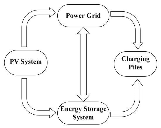
Figure 1.
Energy flow configuration diagram in PE-IES.
In this paper, the PE-IES consists of three parts: the PV system, the energy storage system, and the charging pile, as shown in Figure 2. The core part of the PV system (PV panels) will be laid on the roof of the IEFS building. The inverters will be three sets of inverters, including DC–DC inverters, DC–AC inverters, and AC–DC inverters, respectively. The role of the AC–DC inverters is to deliver energy from the grid to the energy storage system or the charging piles. The role of the DC–DC inverters is to supply the power generated by PV to the station energy storage system, while DC–AC inverters transmit the power generated by PV to the public grid, and in this way, the station can obtain profits from the grid.
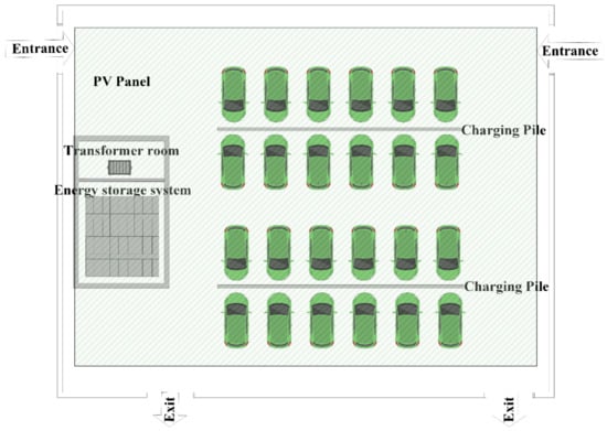
Figure 2.
The composition structure of the PE-IES.
3. Optimized Model Framework
In the PE-IES optimization model, the time-of-day tariff, the EVs charging price for each time interval, the station load status for each time interval, and the PV output for each time interval are used as the input data. Then, the energy flow values of six directions (energy supplied by the PV system to the energy storage system, energy supplied by the PV system to the grid, energy supplied by the energy storage system to the grid, energy supplied by the energy storage system to the charging post, energy supplied by the grid to the energy storage system, and energy supplied by the grid to the charging post, respectively) in each time interval of the station will be solved using the modeling simulation. The decision variables are the energy stored in the energy storage system for each time interval. The values calculated from the decision variables to the six directions of energy flow are presented in Algorithm 1. In addition, this paper applied MOMUS to solve this model.
Algorithm 1 describes the method for converting the decision variables into energy flow values between the systems within the PE-IES.
| Algorithm 1. The transformation process of the decision variables. |
|
3.1. PV System
PV power generation is a technology that uses the PV effect of semiconductors (generally monocrystalline silicon, polycrystalline silicon, and amorphous silicon) to directly convert light energy into electrical energy [29]. PV power generation is known as a non-polluting, cheap, and freely available energy source for human use. PV power generation systems consist of solar panels (the core component), solar controllers, transmission lines, other electrical appliances, etc. The output of photovoltaics can be represented by Equation (1) [30]:
where indicates the PV output power at moment t, is the solar radiation intensity at moment t, is the rated solar radiation, is the rated power of the PV panel, is the generation efficiency, is the temperature coefficient, is the temperature of the environment at moment t, is the temperature of the PV panel under normal conditions, and is the reference temperature of the PV panel. The parameters in Equation (1) are shown in Table 2.
Table 2.
Parameters of the PV system.
3.2. Energy Storage System Model
The energy storage system of the PE-IES can be charged by the public grid and can also supply energy to the charging piles or to the public grid. As shown in Figure 2, the PE-IES model has six energy flow directions. The energy of the storage system comes from the public grid and the PV system, and so the current energy state of the storage system can be expressed by Equation (2):
where is the energy stored in the energy storage system in the time interval, is the amount of electricity supplied by the grid to the energy storage system in the t time interval, is the amount of electricity supplied by the PV system to the energy storage system in the t time interval, is the amount of electricity supplied to the public grid by the energy storage system in the t time interval, is the amount of electricity supplied to the charging piles by the energy storage system in the t time interval, is the charging power of the grid to the energy storage system in the t time interval, is the charging power of PV to the energy storage system in the t time interval, is the discharge power of the energy storage system to the grid, is the discharging power of the energy storage system to the power charging piles, is the discharging power of the energy storage system to the grid, is the discharging power of the energy storage system in the t time interval, is the charging efficiency of the energy storage system, is the discharge efficiency of the energy storage system, and is the time interval, where .
3.3. The Loss Rate of the Energy Storage System Model
The charging or discharging process of the energy storage system of the PE-IES will bring losses to the energy storage system. In order to extend the life of the energy storage system and reduce the losses, it is necessary to model the losses of the energy storage system to calculate the current loss state of the energy storage system, which can estimate the remaining life of the energy storage system. This paper uses the battery capacity loss model from reference [31], which has been proven to have a high accuracy in calculating the battery loss by the charging behavior of the battery. The battery capacity loss can be represented by Equations (3) and (4):
where is the battery capacity loss rate, is the initial state of battery charging, and is the cumulative battery throughput. , , , , , and are the relevant parameters.
The values of and are determined according to the values of the , as shown in Table 3. The values of the other parameters are shown in Table 4. Please refer to [31] for detailed information on each parameter.
Table 3.
Values of and for the different values.
Table 4.
Parameters in the capacity loss model of the energy storage system.
3.4. Optimization Objectives
3.4.1. Maximize the Daily Revenue of the PE-IES
The first objective was to maximize the daily profit of the PE-IES. The daily profit of the PE-IES can be solved by Equation (5) based on the time-of-day tariff and the EV’s charging price for each time interval:
where is the daily revenues of the PE-IES, is the amount of electricity provided by the public grid to the charging piles in the t time interval, is the amount of electricity supplied by the PV system to the public grid in the t time interval, is the charging price of the EVs in the t time interval, is the electricity price in the t time interval, and is the price at which the station sells electricity to the grid in the t time interval.
3.4.2. Minimize the Peak-to-Valley Difference of the Load in the Regional Grid
When the PE-IES is connected to the grid as a load, it will affect the peak-to-valley difference of the load in the regional grid. In order to reduce the peak-to-valley difference of the load and maintain the safety of the grid, minimizing the peak-to-valley difference of the load in the regional grid was set as the objective, as represented in Equations (6) and (7):
where is the peak-to-valley difference of the load in the regional grid, and is the original load of the regional grid, respectively.
3.4.3. Minimize the Loss Rate of the Energy Storage System
In order to have a longer lifetime for the energy storage system, the third objective was to minimize the loss rate of the energy storage system. In this paper, we only considered the effects of charging and discharging on the capacity of the energy storage system. The energy storage system capacity loss is related to the throughput of the energy storage system’s power. Therefore, the third objective can be defined as the minimum of the cumulative number of charges in the energy storage system, as shown in Equation (8):
where is the total loss rate of the energy storage system in a day, and is the loss rate of the energy storage system in the t time interval. The percentage of the capacity loss of the energy storage system can be calculated by Equations (3) and (4).
3.4.4. Relationship between the Objectives
The PE-IES is profitable in two ways: the first way is to charge EVs, the second way is to sell electricity to the grid. When the daily profit increases, the amount of electricity purchased will also increase, as shown in Equation5. But the second objective function (as displayed in Equation (7)) was to minimize the daily amount of electricity purchased, which inevitably causes a conflict. The third objective was to minimize the loss rate of the energy storage system of the PE-IES (as depicted Equation (8)). However, the loss rate of the energy storage system is related to the amount of charge and discharge of the battery. When the charge and discharge are high, the loss rate of the energy storage system is also high, and in turn lower. It can be seen that the first objective and the third objective will also conflict with one another. In summary, the three objectives in the PE-IES model have an exclusion relationship. The PE-IES should therefore be solved by a multi-objective optimization algorithm.
3.5. Constraints
The PE-IES energy control center develops the optimal operation strategy of the station based on the charging demand of the EVs, the PV output, and the charging and selling price of electricity. However, the following constraints need to be satisfied in the process of dispatching energy.
- (1)
- Energy balance constraints
The amount of energy produced in the PE-IES should be equal to the amount consumed, which can be expressed by Equations (9) and (10):
where is the electricity demanded by EVs in the t time interval, is the electricity produced by the PV system in the t time interval, is the electricity added to the energy storage system, and is the electricity released from the energy storage system.
When the number of EVs exceeds the station capacity in a period, the station cannot provide enough energy to meet the demand of the EVs. The constraint of Equation (11) therefore needs to be satisfied.
- (2)
- Inequality constraints
The power stored in the energy storage system needs to satisfy the constraints, as shown in Equation (12):
where is the maximum storage capacity of the energy storage system, and is the minimum storage capacity of the energy storage system.
- (3)
- Constraints on the state of the energy storage system
The energy storage system cannot have charging and discharging states at the same time. Thus, the following constraints need to be satisfied, as shown in Equations (13)–(16):
where is the charging state of PV to the energy storage system, is the charging state of the public grid to the energy storage system, is the discharging state of the energy storage system to the public grid, and is discharging state of the energy storage system to the charging piles, .
4. Case Study and the Solution Method
4.1. Data Collection
- (1)
- The tariff of grid in each period and the price of charging for EVs
The Beijing time-of-day tariff is shown in Figure 3. It can be seen that the valley period of the public grid tariff was 23:00–7:00. The flat periods of the public grid tariff were 7:00–10:00, 15:00–18:00, and 21:00–22:00, respectively. The peak periods of the public grid tariff were 10:00–15:00 and 18:00–21:00, respectively. The price of EV charging at each time interval and the price of selling electricity from the station to the grid at each time interval will thus be used as the initial data.
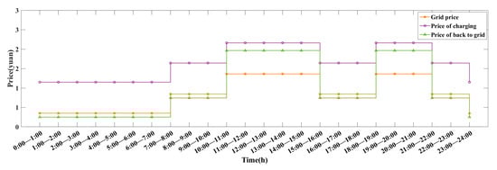
Figure 3.
Tariff of the grid, the price of charging for EVs, and the price of feedback power to the grid.
- (2)
- Load state of the PE-IES
The load of the PE-IES is mainly for charging EVs (private EVs and electric taxis). The general charging time of private EVs was found to be concentrated in the period of 18:00–20:00. Electric taxis charging time was determined to be concentrated at 12:00–14:00 and 23:00–3:00 during the noon break and after work hours, respectively.
It has been assumed that the PE-IES needs to charge 100 vehicles per day, each with a battery capacity of 60 KWh. When the EVs arrive at the station, the battery is assumed to have a residual charge of 10% before charging and 90% after charging, respectively, considering that the battery cannot be overcharged or discharged. The station load is shown in Figure 4.
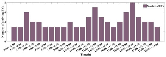
Figure 4.
Number of arriving EVs in different periods.
- (3)
- The PV output
The PV system can only produce energy when light is available. According to Equation (1), the PV system power in the PE-IES can be calculated, as shown in Figure 5.
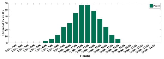
Figure 5.
Energy generation of PV system in each period.
- (4)
- Other basic data in the PE-IES
In the proposed PE-IES, there are 10 charging piles. The power rating of each charging pile is 60 KW. Assuming that the energy storage system can store a maximum of 780 KWh of energy, and that the energy stored in the energy storage system should not be higher than 85% of the maximum capacity and not lower than 15% of the minimum capacity, respectively, the battery capacity of the EV was set to 60 KWh with reference to the Tesla Model 3. The daily load curve of a certain residential area is shown in Figure 6.
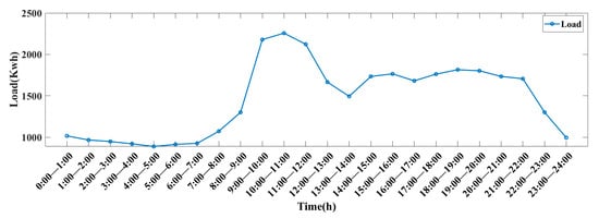
Figure 6.
The daily load curve of the residential area.
4.2. Case Study
In order to analyze the roles of the PV system and the BESS in the PE-IES and verify the effectiveness of the PE-IES, this article simulated the operation of the PE-IES in three different scenarios. The simulation experiments were conducted in MatlabR2020b with the following computer configurations: CPU 2.4GHz, RAM 8.0GB. The specific operating conditions of the three cases are as follows:
Case 1: in this case, there is no PV system or BESS in the PE-IES, meaning that all energy comes from the grid. Without an energy storage system, when a car needs to charge, the PE-IES can only purchase electricity from the grid to meet the EV charging demand. PE-IES is a complete load for the grid. The charging power of the car cannot exceed the maximum charging power of the station, and the specific value can be found in Section 4.1 of this paper. Due to the lack of an energy storage system, the PE-IES model only has two objectives: the maximum daily revenue of the PE-IES, and the minimum load peak-valley difference of the regional grid, respectively.
Case 2: in this case, the PE-IES only has the BESS, and the PV outputs zero in all time periods. Since the grid load is lower in the early morning, the BESS can be charged during this period. When the grid load is higher, the BESS can either be discharged to reduce the amount of electricity purchased by the PE-IES or be directly discharged to the grid to reduce the peak load of the grid. The constraints of the energy storage system can be found in Equations (10)–(12).
Case 3: in this case, the PE-IES has both the PV system and the BESS. Both the grid and the PV system can charge the energy storage system, which can provide energy to the charging stations or to the grid. The grid can also provide energy to the charging stations and the PV system can deliver energy to the grid. The constraints of the PV system and the BESS can be found in Equations (9)–(16). The differences between the above three cases are shown in Table 5.
Table 5.
Comparison of various cases.
MOMUS can be used to calculate all three cases mentioned above. The population size, NP, was 200, and the maximum number of iterations, Tmax, was 200, respectively.
4.3. MOMUS
The PE-IES model is a complex model with three objectives and multiple constraints. Therefore, the algorithm needs to encompass a stronger search capability when solving this model. Both the MFO and BWO algorithms have an excellent global search capability and local search capability. The MOMUS algorithm learns from the spiral search approach of the MFO algorithm and the linear search approach of the BWOA, respectively. The Levy strategy was introduced into the MOMUS algorithm in order to avoid falling into the local optima during the search process. The main steps for solving the PE-IES model using the MOMUS algorithm are as follows:
Step 1: generate the parent population , advantageous population , the maximum number of iterations , initial data of PE-IES energy dispatching model, etc.
Step 2: four individuals , , and will be selected from the parent population , and the advantageous population according to the number of iterations.
When the algorithm is in the first iteration, four different individuals , , and are selected in the population .
When the algorithm is not in the first iteration, any two different individuals, e.g., , are selected in population , and any two different individuals, e.g., , are selected from population , respectively.
Step 3: generate three random numbers, e.g., , , and , and choose different update formulas according to the following conditions.
When < 0.7 and < 0.7, the individual performs the position update with Equation (17):
where is the individual after the location update, and is a parameter that takes the values 0 or 1.
When < 0.7 and ≥ 0.7, the individual performs the position update with Equation (18):
where is an individual and is another individual.
When ≥ 0.7 and < 0.9, the individual performs the position update with Equation (19):
where denotes an individual in population , and , and are parameters in the location update equation, and can be expressed in Equations (20)–(23):
where is a random number between 0 and 1, respectively, and is the number of current iterations.
When ≥ 0.7 and ≥ 0.9, the individual can perform the position update with Equation (24):
where represents the levy flight formula and is the dimension of the decision variable.
Step 4: place individuals with updated positions in the offspring population . .
Execute Algorithm 1 (calculate the value of the energy transferred between the systems of the PE-IES according to the state of the energy storage system).
The combined population is sorted non-dominantly, and all individuals are stratified () according to their solutions. All individuals in stratum are placed in population .
Step 5: the number of individuals in each layer is added until , and the current cumulative number of layer is recorded as .
If , then all individuals in layers are placed in the offspring population.
If , all individuals in the layer are normalized using Equations (25)–(27), and reference points are generated:
where is the intercept between the axis of the ith target and the linear hyper-plane; is the number of objective functions, is the minimum value of the ith objective function in solution set ,, and is the ith transformed objective.
Step 6: the vertical distances between all individuals in the layer and each reference point are calculated, and all individuals in the layer are connected to the nearest reference point, where the vertical distances can be calculated by Equation (28).
Step 7: the number of individuals associated with the reference point is calculated, which can be represented as . The number of individuals selected is calculated from , which can be denoted as .
Step 8: randomly select a non-repeating reference point. And if , the individual with the smallest vertical distance from the selected reference point is selected. If all reference points , but , then individuals with the reference point will be selected.
Step 9: repeat steps 2–8 until the Tmax has been reached.
Algorithm 2 mainly describes the complete process of solving the PE-IES optimization model using MOMUS. The objective functions of the PE-IES optimization model will be used as the fitness functions.
| Algorithm 2. The complete process of the MOMUS algorithm. |
Input: Define the initial number of population (), the maximum number of iterations (Tmax), the input data of the PE-IES model, such as tariff of the grid, number of arriving EVs, etc.
|
The flow chart of the MOMUS algorithm for solving the PE-IES energy optimal dispatching model is shown in Figure 7.
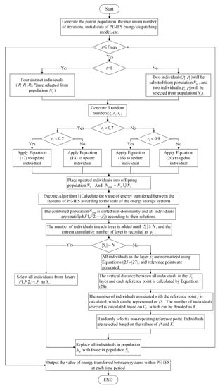
Figure 7.
Flow chart of solving PE-IES using the MOMUS algorithm.
5. Results and Discussion
5.1. Results Analysis
In Case 1, the station becomes a complete load on the grid due to there being no PV system and no energy storage system. The revenue comes from the difference between the station’s purchase price of electricity from the grid and the price of charging the EVs. The amount of electricity purchased from the grid for each time interval at the station is the same as the amount of electricity demanded by the EVs. Since there is no energy storage system in the station, the loss of the energy storage system is 0. Figure 8 shows the profit for each time interval and cumulative profit. Figure 9 shows the amount of electricity purchased for each time interval and the final load of the grid in that area. It can be seen from Figure 9 that after the PE-IES is powered by the regional grid of a certain residential area, the load in each time period of the residential area increased.
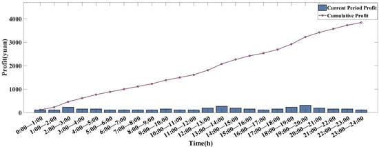
Figure 8.
Profit and cumulative profit of the PE-IES for each period in Case 1.
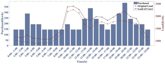
Figure 9.
Amount of electricity purchased in the PE-IES (left Y-axis) and the load in each time period of the regional grid (right Y-axis) in Case 1.
In Case 2, the integrated energy station contains an energy storage system. When the grid load is low, the energy storage system can be charged during this period, which can reduce the energy waste from the grid. When the grid load is high, the energy storage system can be discharged during this period, which can thereby reduce the amount of electricity purchased. The above method can be used to carry out peak shaving and valley filling of the regional grid.
In this case, the results of the operation is shown in Figure 10. After using the entropy weight method to determine the weights of each objective function as 0.35, 0.34, and 0.31, respectively, a set of solutions were selected from the Pareto set (with objective 1 = −4811.9, objective 2 = 1011.67, and objective 3 = 0.0871%, respectively). The purchased power of the PE-IES in each time period is shown in Figure 11, and the load status of the regional grid is shown in Figure 12, respectively.
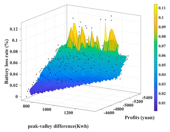
Figure 10.
The Pareto solution set of PE-IES in Case 2 solved using the MOMUS algorithm.
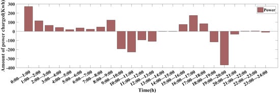
Figure 11.
Charging and discharging of the PE-IES’ energy storage system in each period in Case 2.
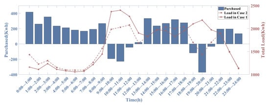
Figure 12.
Amount of electricity purchased in the PE-IES (left Y-axis) and the load in each time period of the regional grid (right Y-axis) in Case 2.
From Figure 11, it can be observed that the energy storage system charges during periods of low-grid load (0:00–9:00, and 17:00–18:00, respectively), while discharging during periods of high-grid load (9:00–13:00, and 18:00–21:00, respectively). It can be inferred from Figure 11 and Figure 12 that the PE-IES can use the energy storage system to meet the charging needs of the EVs on-site while peak shaving and valley filling the regional grid. In addition, Figure 12 compares the final load curves of the regional grid in Case 1 and Case 2, where the peak-valley differences of Case 1 and Case 2 are 1343 and 1011.67, respectively. The peak-valley difference of Case 2 decreased by 24.67% compared to Case 1.
Case 3 is the PE-IES model proposed in this paper. The revenue comes from the difference between the station’s purchase price of electricity from the grid and the price of charging the EVs. The PV system and the energy storage system that delivers energy to the grid can also generate revenue. The energy storage system obtains energy not only from the grid but also from the PV system. The results of Case 3 are shown in Figure 13.
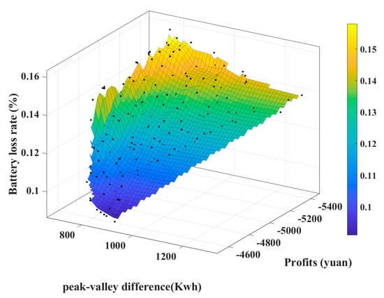
Figure 13.
The Pareto solution set of PE-IES in Case 3 solved using the MOMUS algorithm.
The weights of each objective were determined using the entropy weight method as 0.36, 0.33, and 0.31, respectively, and a set of solutions were selected from the Pareto set (with objective 1 = −4861.9, objective 2 = 932.75, and objective 3 = 0.1002%, respectively). The purchased power of the PE-IES in each time period is shown in Figure 14, and the load status of the regional grid is shown in Figure 15, respectively.
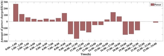
Figure 14.
Charging and discharging of the PE-IES’ energy storage system in each period in Case 3.
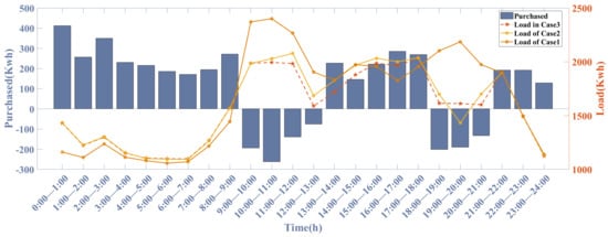
Figure 15.
Amount of electricity purchased in the PE-IES (left Y-axis) and the load in each time period of the regional grid (right Y-axis) in Case 3.
In Case 3, the energy storage system loss rate increased by 15.04% compared to Case 2. However, the daily profit increased by 1.04% and 26.61% compared to Case 2 and Case 1, respectively. The peak-to-valley difference of the load in the regional grid decreased by 7.80% and 30.54% compared to Case 2 and Case 1, respectively. The daily revenues in Case 3 were found to be higher than those in Case 2. The first reason for this was that the PV systems reduce the amount of electricity purchased at the station, which ultimately reduces the cost of electricity purchased. The second reason was that the PV system delivers the generated energy to the grid, which subsequently adds revenues to the station. The loss rate of the energy storage system in Case 3 was found to be higher than that in Case 2. As the energy generated by the PV system in Case 3 will be preferentially delivered to the energy storage system, the charge and discharge of the energy storage system will be increased. Eventually, the loss rate of the energy storage system will further increase as a result.
Based on the above three cases, we can draw the following conclusions. The energy storage system can be charged when the grid load is low, and discharged when the grid load is high, which will reduce the peak-to-valley difference of the load in the regional grid. Combined with the energy storage system and the PV system, the loss rate of the energy storage system will increase. But it can also further reduce the peak-valley difference of the regional grid, and increase the daily revenues of the station as a result.
5.2. Algorithm Comparison
To demonstrate the effectiveness of the MOMUS algorithm, eight algorithms (adaptive NSGA-III (ANSGA-III) [32], bi-Goal Evolution (BIGE) [33], effective θ-dominance-based evolutionary algorithm (θ-DEA) [34], knee point-driven evolutionary algorithm (KNEA) [35], NSGA-III [22], a reference points-based evolutionary algorithm (RPEA) [36], a strength Pareto evolutionary algorithm based on reference direction (SPEAR) [37], and the MOMUS algorithm) were applied in the experiments to calculate the PE-IES optimal dispatching model. Each algorithm was run 10 times. Figure 16 show the results of applying these eight algorithms to solve the PE-IES model, respectively.
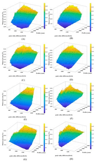
Figure 16.
The Pareto solution sets obtained by solving the PE-IES using eight different algorithms. (A) Results of ANSGA-Ⅲ; (B) Results of BIGE; (C) Results of KNEA; (D) Results of NSGA-Ⅲ; (E) Results of RPEA; (F) Results of SPEAR; (G) Results of θ-DEA; and (H) Results of MOMUS.
In order to compare the performance of the algorithms in solving the model, Table 6, Table 7 and Table 8 give the comparison results of three metrics (spread, HV, and runtime) for each of the eight algorithms. Each of these algorithms was run 10 times, and the best, worst, and average values of results are shown. Spread and HV were calculated as follows.
Table 6.
Comparison of the metric spread.
Table 7.
Comparison of the metric HV.
Table 8.
Comparison of the metric runtime(s).
(1) Spread: This metric indicates the distributivity of the solution set in the space of the feasible domains [38]. When the value of spread is smaller, it proves that the distributivity of the solution set in the space is stronger. It can be determined using Equation (29):
where and are the Euclidean distances between the extremal and boundary solutions of the non-dominated solution set; is the number of solutions in the non-dominated solution set found by the algorithm; is the Euclidean distance between adjacent solutions in the non-dominated solution set; and is the average of all .
(2) Hypervolume (HV): the hypervolume consisting of the position of the solution set in the feasible domain space and the position of the reference point [39]. When the HV is larger, it indicates the better performance of the algorithm. It can be calculated using Equation (30):
where is the number of solutions in the non-dominated solution set, and is the hypervolume formed by the ith solution and the reference point in the non-dominated solution set.
(3) Runtime: how long the algorithm takes to compute the problem. The larger the runtime, the longer the runtime of the algorithm.
HV and spread are two evaluation indicators for measuring the quality of the solutions obtained by these algorithms. The HV indicator represents the volume of the region enclosed by the non-dominated solution set obtained by the algorithm and the reference point in the objective space. A larger HV value indicates a better overall performance of the algorithm. The spread indicator is often used as a measure of the diversity of the solutions generated by an algorithm. In the process of solving the PE-IES, a smaller spread value indicates a better overall performance of the algorithm. From the data in Table 7, compared with the other seven algorithms, the runtime of the MOMUS algorithm was shorter, which shows that the computational complexity of the MOMUS algorithm is smaller. From the data in Table 6, Table 7 and Table 8, it is clear that the set of non-dominated solutions computed by the MOMUS algorithm has a better overall performance compared to the seven other algorithms. Overall, it has been demonstrated from this study that MOMUS outperforms the other seven algorithms in terms of performance.
In Case 1, the PE-IES does not have a PV system nor a BESS, which is a traditional electric vehicle charging station. In Case 2, the PE-IES does not have a PV system and includes a BESS for energy storage. From Figure 9 and Figure 12, it can be observed that compared to the load peak-valley difference of the regional grid in Case 1, the load peak-valley difference of the regional grid in Case 2 decreased by 24.67%, and the profit increased by 26.25%, respectively. Since Case 1 does not have a BESS, the energy loss of the energy storage system in Case 2 increased by 0.0871%. As can be seen from this, energy storage systems can not only store excess energy during periods of low demand and release it during peak periods to smooth out the load on the grid and reduce its burden, but they can also reduce electricity costs by storing energy during periods of low demand and releasing it during peak periods. Furthermore, energy storage systems can generate additional revenue for the charging station by selling excess energy back to the grid. In Case 3, the PE-IES is a complete model that includes both the PV system and the BESS. From Figure 15, it can be seen that the PE-IES in Case 3 increased its profits by 26.61% and reduced the load peak-valley difference of the regional grid by 30.54%, respectively, compared to the PE-IES in Case 1. In Case 3, the PE-IES has a PV system in addition to the BESS compared to the PE-IES in Case 2. The loss rate of the energy storage system in Case 3 was higher than that in Case 2. As the energy generated by the PV system in Case 3 will be preferentially delivered to the energy storage system, the charge and discharge of the energy storage system will increase as a result. However, the daily profit increased by 1.04%, and the load peak valley difference of the regional grid was reduced by 7.80%, respectively. From this, it can be seen that adding a PV system can reduce the purchase cost of electricity for the PE-IES, and excess electricity can be sold to the grid to reduce the load peak-valley difference of the grid, ultimately maintaining the stability of the grid operation.
Furthermore, this paper proposed a new many-objective optimization algorithm based on multi-updating strategies. MOMUS was compared with ANSGA-III, BIGE, θ-DEA, KNEA, NSGA-III, SRPEA, and PEAR under the same conditions using evaluation metrics, such as HV, spread, and runtime. The results confirmed that MOMUS achieves a higher quality Pareto front solutions compared to the other algorithms.
6. Conclusions
The large-scale charging of EVs imposes an additional load on the grid, which may lead to an increased instability in the power system. It is necessary to balance the load on the grid and prevent it from affecting the peak-to-valley difference in the grid. At the same time, for EV charging stations, it is important to consider how to meet the charging demand, utilize renewable energy resources effectively, and manage the energy storage and distribution of the charging stations. Therefore, this article introduces the PV system and BESS into the charging station to form a PE-IES. This paper considers the PV output at different time periods, electricity prices at different time periods, the number of charging vehicles at different time periods, and the regional grid load at different time periods. A multi-objective optimization model for PE-IES was also established. The goal was to meet the charging demand for electric vehicles while considering the loss rate of the BESS, ultimately improving the daily profit of the PE-IES and reducing the peak-to-valley difference of the load in the regional grid. After conducting simulation experiments in the three cases, the results indicate that compared to the traditional charging station, the daily profit of the PE-IES will increase by 26.61%, and the peak-to-valley difference of the load in the regional grid will decrease by 30.54%, respectively. The validity of the model was also proven. Furthermore, this paper proposed a new algorithm (MOMUS) to solve the PE-IES model. MOMUS was compared with seven other algorithms in terms of the evaluation metrics HV, spread, and runtime. The obtained results confirm that MOMUS outperforms the other algorithms in terms of its optimization performance. In the future, the joint optimal scheduling of all PE-IESs in the region will be the focus of the work.
Author Contributions
X.L.: Investigation, experimentation, data curation, methodology and supervision. B.Q.: Investigation, experimentation, data curation, writing—original draft and writing—review and editing. Z.J.: Investigation, data curation, and validation. B.F.: Conceptualization, Validation and investigation. H.H.: Conceptualization, Validation and investigation. All authors have read and agreed to the published version of the manuscript.
Funding
National Natural Science Foundation of China, grant number 51809097; and Open Foundation of Hubei Engineering Research Center for Safety Monitoring of New Energy and Power Grid Equipment, grant number HBSKF202125.
Data Availability Statement
Data available on request due to restrictions, e.g., privacy or ethical.
Acknowledgments
The author would appreciate the support of the National Natural Science Foundation of China (51809097) and the Open Foundation of Hubei Engineering Research Center for Safety Monitoring of New Energy and Power Grid Equipment (HBSKF202125) and the help of the editor and reviewers.
Conflicts of Interest
The authors declare no conflict of interest.
References
- Kene, R.O.; Olwal, T.O. Energy Management and Optimization of Large-Scale Electric Vehicle Charging on the Grid. World Electr. Veh. J. 2023, 14, 95. [Google Scholar] [CrossRef]
- Kene, R.; Olwal, T.; van Wyk, B.J. Sustainable Electric Vehicle Transportation. Sustainability 2021, 13, 12379. [Google Scholar] [CrossRef]
- Qiao, Y.; Hu, F.; Xiong, W.; Guo, Z.; Zhou, X.; Li, Y. Multi-objective optimization of integrated energy system considering installation configuration. Energy 2022, 263, 12578. (In English) [Google Scholar] [CrossRef]
- Lv, D.; Tang, J.; Yang, C. A Multi-objective Optimal Dispatch Method for Integrated Energy System Considering Multiple Loads Variations. E3S Web Conf. 2021, 256, 02025. [Google Scholar] [CrossRef]
- Kou, Y.N.; Zheng, J.H.; Li, Z.; Wu, Q.H. Many-objective optimization for coordinated operation of integrated electricity and gas network. J. Mod. Power Syst. Clean Energy 2017, 5, 350–363. (In English) [Google Scholar] [CrossRef]
- Saner, C.B.; Trivedi, A.; Srinivasan, D. A Cooperative Hierarchical Multi-Agent System for EV Charging Scheduling in Presence of Multiple Charging Stations. IEEE Trans. Smart Grid 2022, 13, 2218–2233. (In English) [Google Scholar] [CrossRef]
- Su, S.; Wei, C.; Li, Z.; Xia, M.; Chen, Q. Critical load restoration in coupled power distribution and traffic networks considering spatio-temporal scheduling of electric vehicles. Int. J. Electr. Power Energy Syst. 2022, 141, 108180. [Google Scholar] [CrossRef]
- Zhao, Z.; Lee, C.K.M. Dynamic Pricing for EV Charging Stations: A Deep Reinforcement Learning Approach. IEEE Trans. Transp. Electrif. 2022, 8, 2456–2468. [Google Scholar] [CrossRef]
- Wu, Z.; Chen, B. Distributed Electric Vehicle Charging Scheduling with Transactive Energy Management. Energies 2022, 15, 163. (In English) [Google Scholar] [CrossRef]
- Dai, Q.; Liu, J.; Wei, Q. Optimal Photovoltaic/Battery Energy Storage/Electric Vehicle Charging Station Design Based on Multi-Agent Particle Swarm Optimization Algorithm. Sustainability 2019, 11, 1973. (In English) [Google Scholar] [CrossRef]
- Javed, M.S.; Song, A.; Ma, T. Techno-economic assessment of a stand-alone hybrid solar-wind-battery system for a remote island using genetic algorithm. Energy 2019, 176, 704–717. (In English) [Google Scholar] [CrossRef]
- Zhang, X.; Zheng, L. Coordinated dispatch of the wind-thermal power system by optimizing electric vehicle charging. Clust. Comput. 2019, 22, 8835–8845. (In English) [Google Scholar] [CrossRef]
- Hao, Y.; Dong, L.; Liang, J.; Liao, X.; Wang, L.; Shi, L. Power forecasting-based coordination dispatch of PV power generation and electric vehicles charging in microgrid. Renew. Energy 2020, 155, 1191–1210. (In English) [Google Scholar] [CrossRef]
- Shojaabadi, S.; Talavat, V.; Galvani, S. A game theory-based price bidding strategy for electric vehicle aggregators in the presence of wind power producers. Renew. Energy 2022, 193, 407–417. (In English) [Google Scholar] [CrossRef]
- Dukpa, A.; Butrylo, B. MILP-Based Profit Maximization of Electric Vehicle Charging Station Based on Solar and EV Arrival Forecasts. Energies 2022, 15, 5760. (In English) [Google Scholar] [CrossRef]
- Shi, R.; Zhang, P.; Zhang, J.; Niu, L.; Han, X. Multidispatch for Microgrid including Renewable Energy and Electric Vehicles with Robust Optimization Algorithm. Energies 2020, 13, 2813. (In English) [Google Scholar] [CrossRef]
- Kerdphol, T.; Fuji, K.; Mitani, Y.; Watanabe, M.; Qudaih, Y. Optimization of a battery energy storage system using particle swarm optimization for stand-alone microgrids. Int. J. Electr. Power Energy Syst. 2016, 81, 32–39. (In English) [Google Scholar] [CrossRef]
- El-Taweel, N.A.; Farag, H.E.; Shaaban, M.F.; AlSharidah, M.E. Optimization Model for EV Charging Stations With PV Farm Transactive Energy. IEEE Trans. Ind. Inform. 2022, 18, 4608–4621. (In English) [Google Scholar] [CrossRef]
- Prajapati, S.; Fernandez, E. Solar PV parking lots to maximize charge operator profit for EV charging with minimum grid power purchase. Energy Sources Part A Recover. Util. Environ. Eff. 2020. (In English) [Google Scholar] [CrossRef]
- Wen, L.; Zhou, K.; Yang, S.; Lu, X. Optimal load dispatch of community microgrid with deep learning based solar power and load forecasting. Energy 2019, 171, 1053–1065. (In English) [Google Scholar] [CrossRef]
- Amiri, S.S.; Jadid, S.; Saboori, H. Multi-objective optimum charging management of electric vehicles through battery swapping stations. Energy 2018, 165, 549–562. [Google Scholar] [CrossRef]
- Deb, K.; Jain, H. An Evolutionary Many-Objective Optimization Algorithm Using Reference-Point-Based Nondominated Sorting Approach, Part I: Solving Problems With Box Constraints. IEEE Trans. Evol. Comput. 2014, 18, 577–601. [Google Scholar] [CrossRef]
- Cui, Z.; Chang, Y.; Zhang, J.; Cai, X.; Zhang, W. Improved NSGA-III with selection-and-elimination operator. Swarm Evol. Comput. 2019, 49, 23–33. [Google Scholar] [CrossRef]
- De Oliveira, M.C.; Delgado, M.R.; Britto, A. A hybrid greedy indicator- and Pareto-based many-objective evolutionary algorithm. Appl. Intell. 2021, 51, 4330–4352. [Google Scholar] [CrossRef]
- Li, K.; Yan, X.; Han, Y.; Ge, F.; Jiang, Y. Many-objective optimization based path planning of multiple UAVs in oilfield inspection. Appl. Intell. 2022, 52, 12668–12683. [Google Scholar] [CrossRef]
- Gu, Z.-M.; Wang, G.-G. Improving NSGA-III algorithms with information feedback models for large-scale many-objective optimization. Future Gener. Comput. Syst.-Int. J. Escience 2020, 107, 49–69. [Google Scholar] [CrossRef]
- Peña-Delgado, A.F.; Peraza-Vázquez, H.; Almazán-Covarrubias, J.H.; Torres Cruz, N.; García-Vite, P.M.; Morales-Cepeda, A.B.; Ramirez-Arredondo, J.M. A Novel Bio-Inspired Algorithm Applied to Selective Harmonic Elimination in a Three-Phase Eleven-Level Inverter. Math. Probl. Eng. 2020, 2020, 8856040. [Google Scholar] [CrossRef]
- Mirjalili, S. Moth-flame optimization algorithm: A novel nature-inspired heuristic paradigm. Knowl. Based Syst. 2015, 89, 228–249. [Google Scholar] [CrossRef]
- Hernández, J.; Sanchez-Sutil, F.; Muñoz-Rodríguez, F.; Baier, C. Optimal sizing and management strategy for PV household-prosumers with self-consumption/sufficiency enhancement and provision of frequency containment reserve. Appl. Energy 2020, 277, 115529. [Google Scholar] [CrossRef]
- Sun, B.J. A multi-objective optimization model for fast electric vehicle charging stations with wind, PV power and energy storage. J. Clean. Prod. 2021, 288, 125564. (In English) [Google Scholar] [CrossRef]
- Suri, G.; Onori, S. A control-oriented cycle-life model for hybrid electric vehicle lithium-ion batteries. Energy 2016, 96, 644–653. [Google Scholar] [CrossRef]
- Jain, H.; Deb, K. An Evolutionary Many-Objective Optimization Algorithm Using Reference-Point Based Nondominated Sorting Approach, Part II: Handling Constraints and Extending to an Adaptive Approach. IEEE Trans. Evol. Comput. 2014, 18, 602–622. [Google Scholar] [CrossRef]
- Li, M.; Yang, S.; Liu, X. Bi-goal evolution for many-objective optimization problems. Artif. Intell. 2015, 228, 45–65. [Google Scholar] [CrossRef]
- Yuan, Y.; Xu, H.; Wang, B.; Yao, X. A New Dominance Relation-Based Evolutionary Algorithm for Many-Objective Optimization. IEEE Trans. Evol. Comput. 2016, 20, 16–37. [Google Scholar] [CrossRef]
- Zhang, X.; Tian, Y.; Jin, Y. A Knee Point-Driven Evolutionary Algorithm for Many-Objective Optimization. IEEE Trans. Evol. Comput. 2015, 19, 761–776. [Google Scholar] [CrossRef]
- Liu, Y.; Gong, D.; Sun, X.; Zhang, Y. Many-objective evolutionary optimization based on reference points. Appl. Soft Comput. 2017, 50, 344–355. [Google Scholar] [CrossRef]
- Jiang, S.; Yang, S. A Strength Pareto Evolutionary Algorithm Based on Reference Direction for Multiobjective and Many-Objective Optimization. IEEE Trans. Evol. Comput. 2017, 21, 329–346. [Google Scholar] [CrossRef]
- Deb, K.; Pratap, A.; Agarwal, S.; Meyarivan, T. A fast and elitist multiobjective genetic algorithm: NSGA-II. IEEE Trans. Evol. Comput. 2002, 6, 182–197. [Google Scholar] [CrossRef]
- Brest, J.; Greiner, S.; Boskovic, B.; Mernik, M.; Zumer, V. Self-Adapting Control Parameters in Differential Evolution: A Comparative Study on Numerical Benchmark Problems. IEEE Trans. Evol. Comput. 2006, 10, 646–657. [Google Scholar] [CrossRef]


Disclaimer/Publisher’s Note: The statements, opinions and data contained in all publications are solely those of the individual author(s) and contributor(s) and not of MDPI and/or the editor(s). MDPI and/or the editor(s) disclaim responsibility for any injury to people or property resulting from any ideas, methods, instructions or products referred to in the content. |
© 2023 by the authors. Licensee MDPI, Basel, Switzerland. This article is an open access article distributed under the terms and conditions of the Creative Commons Attribution (CC BY) license (https://creativecommons.org/licenses/by/4.0/).