Energy Forecasting Model for Ground Movement Operation in Green Airport

Abstract

The aviation industry has driven economic growth and facilitated cultural exchange over the past century. However, concerns have arisen regarding its contribution to greenhouse gas emissions and potential impact on climate change. In response to this challenge, stakeholders have proposed the use of electric ground support vehicles, powered by renewable energy sources, at airports. This solution aims to not only reduce emissions, but to also lower energy costs. Nonetheless, the successful implementation of such a system relies on accurate energy demand forecasting, which is influenced by flight data and fluctuations in renewable energy availability. This paper presents a novel data-driven, machine-learning-based energy prediction model that compared the performance of the Facebook Prophet and vector autoregressive integrated moving average algorithms to develop time series models to forecast the ground movement operation net energy demand in the airport, using historical flight data and an onsite airport-based PV power system (ASPV). The results demonstrate the superiority of the Facebook Prophet model over the vector autoregressive integrated moving average (VARIMA), highlighting its utility for airport operators and planners in managing energy consumption and preparing for future electrified ground movement operations at the airport.

1. Introduction

The concept of a green airport can be classified under both the green transport plan (GTP) and green architecture plan (GAP), using a range of renewable energy and energy-efficient technologies [1]. The term “green airport” refers to a number of creative initiatives that improve the overall environmental performance of airport operations, intermodal transportation of people and goods between airports, and airport infrastructure. These initiatives include electrification and the use of renewable energy sources. An airport with a green concept reduces GHG emissions and improves energy efficiency and surface accessibility by integrating new concepts in public transportation [2].

Green airports have become increasingly popular in recent years as the aviation industry aims to reduce its carbon footprint and improve sustainability [2]. Energy forecasting is an essential task in green airports, as it helps to optimize energy production and consumption, reduce costs, and improve energy efficiency [3]. Additionally, electric utilities and energy management systems, such as grid operators, use energy forecasting models to predict the electricity demand required to balance the generation and load demand [4]. This process involves estimating the future load demand to ensure the reliable operation of the electric grid. Energy forecasting is essential for power system planners and grid operators to guarantee sufficient electricity generation to meet future demand [5].

Moreover, load forecasting is essential for other participants in the electric energy generation, transmission, and distribution systems. It helps in capacity expansion, better grid operation, budget planning, maintenance scheduling, and fuel management [6]. Forecasting is also employed in various fields, such as finance, to predict stock exchange courses, business to manage inventory, and forecast demand; medicine, to monitor the spread of diseases; and meteorology, for weather forecasting [7]. Forecasting is the process of predicting future outcomes by analysing trends in past and present data [8]. It comprises three main components: input variables (past and present data), forecasting/estimation methods (analysis of trends), and output variables (future predictions), as illustrated in Figure 1.

Forecasted models can cover a range of time frames, from a few hours to as long as 100 years [9]. Ref. [10] proposed that short-term forecasts cover a period of five years or less, medium-term forecasts range between three and fifteen years, and long-term forecasts span ten years or more. However, this categorization can confuse medium- and long-term projections because of their overlapping time frames. To avoid this confusion, Ref. [9] defines time span or modelling horizons as follows: short-term (t < 3 years), medium-term (between 3 and 15 years inclusive), and long-term (more than 15 years), where t represents the time span in years.

Forecasting techniques used for trend analysis can be broadly classified into two main types: stand-alone and hybrid. Stand-alone methods use a single technique for trend analysis, while hybrid methods integrate more than one stand-alone technique. Stand-alone methods can be further classified into statistical, computational intelligence (CI), and mathematical programming (MP). Hybridization is typically used to improve the reliability and accuracy of forecast output [7]. Hybrid methods are divided into four categories: statistical–statistical, statistical–CI, CI–CI, and statistical–MP methods. In addition, some studies in the literature use multiple stand-alone and/or hybrid methods for comparison and critique purposes [9].

Past research on forecasting methods in energy planning has traditionally been divided into either application areas or categories of underlying techniques. However, the evolution of application areas and new techniques have made these categorizations inflexible and incomplete [11]. For example, application-based categorizations have not fully accommodated the importance of behavioural energy conservation in the climate and energy debate. Similarly, dividing forecasting methods into statistical and AI-based approaches is inaccurate and insufficient, as hybrid methods that combine both approaches are increasingly common [9].

Research has indicated that hybrid methods are more effective in forecasting nonlinear and discontinuous data, especially when the relationship between variables is unknown and difficult to handle statistically [12,13,14,15]. However, it is worth noting that hybrid machine-learning methods can be more complex in both learning and application than statistical methods. Consequently, the learning complexity of a method can influence the choice of forecasting technique [16]. In addition, data availability is also a crucial factor to consider when choosing a forecasting method. For example, artificial neural networks (ANNs) are data-driven and require a large dataset for higher forecasting accuracy [17]. In incomplete data sets, fuzzy logic may be more suitable. However, the level of accuracy with fuzzy logic may not always be satisfactory [17]. Grey prediction is another useful method, particularly when dealing with uncertainty problems, small sample sizes, and incomplete or discrete data [15,18].

Many researchers advocate for the use of hybridization methods to improve the accuracy of forecasting models [19,20]. Ref. [21] discusses the challenges faced by various country-driven sectors due to the COVID-19 pandemic, highlighting the lessons learned from these challenges. The paper provides a roadmap for future forecasting in these sectors, emphasizing the importance of accurate data and the use of appropriate forecasting methods. The sectors covered in the paper include healthcare, tourism, education, finance, and trade.

The authors in [22] proposed a hybrid approach combining machine learning and statistical methods to improve the accuracy of forecasting models. However, they note that this can increase the complexity of the models. The paper emphasizes the significance of integrating predictions from dynamic models and machine learning models to improve forecasting accuracy. The hybrid forecasting approach presented in the study offers a valuable framework for combining the strengths of statistical and machine learning techniques. The empirical evaluations demonstrate the superiority of the hybrid model over individual models. The paper provides insights into the advantages and challenges of the hybrid approach, and highlights its potential for enhancing forecasting capabilities in various domains.

Time Series Forecasting

Time series algorithms have been widely used in energy forecasting tasks due to their ability to capture the patterns and trends in time series data. The technique is used to predict future values of a variable based on its past behaviour. Popular models for time series forecasting include autoregressive integrated moving average (ARIMA) [23], exponential smoothing (ETS) [24], vector autoregression (VAR), seasonal autoregressive integrated moving average (SARIMA) [25], and long short-term memory (LSTM) [26]. These models can handle both stationary and non-stationary time series data, and have been widely used in various fields such as finance, economics, energy, and weather forecasting [27,28].

Ref. [29] presents a study on energy consumption forecasting in China using an ARIMA model. The research aims to provide accurate energy consumption predictions to support energy management and decision-making. The study uses historical data on energy consumption in China from 1995 to 2019 and employs the Box–Jenkins approach to build an ARIMA model. The model is then used to forecast energy consumption from 2020 to 2025. The results of the study show that the VARIMA model is an effective tool for energy consumption forecasting in China, and can provide accurate predictions with a high degree of confidence.

Ref. [30] evaluates the accuracy of prediction models for airport passenger throughput using a hybrid approach. The main objective of this study is to identify the most effective model for predicting airport passenger traffic, which holds significant importance for airport management and planning. To achieve this, historical data on passenger throughput at an international airport in China from 2015 to 2019 are utilized, and the performance of four prediction models, namely ARIMA, LSTM, SVM, and a hybrid model, is compared.

The results of the study reveal that the hybrid model surpasses the other models in terms of prediction accuracy. In addition, it exhibits a lower mean absolute percentage error (MAPE) and a higher correlation coefficient (R), indicating its superior performance in accurately predicting airport passenger traffic.

Ref. [31] proposes a machine-learning approach for predicting the energy consumption of ships in a port, taking into account the concept of green ports. The method considers various factors that influence energy consumption, such as weather, traffic, and operational characteristics of the ship, and uses data from port monitoring systems and ship sensors. The proposed model uses a random forest algorithm for prediction, and is validated using real-world data from Jing Tang Port in China. The results show that the model has high accuracy and can be used to support decision-making for energy-efficient operations in green ports.

Ref. [32] proposes a hybrid model for predicting water levels in the Red Hills Reservoir, using a combination of seasonal autoregressive integrated moving averages (SARIMA) and artificial neural network (ANN) models. The approach uses time series analysis to identify trends, seasonality, and noise in the data, and capture the seasonal patterns in the data. The hybrid model is evaluated using real-world data from the Red Hills Reservoir in India, and compared with several benchmark models. The results show that the proposed model outperforms other models in terms of accuracy, and can be used for real-time water level prediction and management. However, traditional time series forecasting methods, such as ARIMA and exponential smoothing, have limitations in handling the complexity of energy data, which is often characterized by nonlinear relationships, seasonality, and multiple variables.

In addition, traditional time series forecasting methods require expert knowledge and manual tuning of hyperparameters to achieve accurate results, which can be time-consuming and error-prone [33]. Therefore, further research has focused on developing new algorithms and improving existing ones to handle more complex time series data.

The Facebook Prophet algorithm addresses these limitations by incorporating a flexible Bayesian framework that automatically selects the appropriate model parameters, allowing non-experts to use it easily. It also includes a customizable seasonal component that can capture multiple seasonal patterns, and a robust regression model that handles outliers and missing values [34]. Furthermore, the algorithm provides interpretable results that help users understand the drivers of change in their data and make informed decisions. As a result, it has been shown to outperform traditional time series methods in various applications, including retail sales, energy demand, and financial forecasting [33,35]. Its ability to handle multiple seasonalities, user-friendly and easily interpretable nature, robustness to missing data and outliers, flexibility in modelling trend changes, and scalability make it a valuable tool for optimizing energy usage in green airports. In addition, the Facebook Prophet algorithm takes into account various factors, such as holidays, seasons, and events, that affect the predicted variables, resulting in more accurate forecasts. However, from the literature review above, there is no work in the scientific literature on forecasting the energy consumption of ground support equipment operations at airports.

This study developed an energy prediction model using the machine-learning-based Facebook Prophet algorithm tools in Python to forecast future ground operation energy demand in the airport. The model’s time series multivariate algorithm forecasts and merges the EGSEs charging load demand with the onsite PV power system output to optimize the power flow in the airport.

This study is the first to apply Facebook’s Prophet model in the context of energy demand forecasting for optimizing airport ground movement operations. It builds upon previous research in time series forecasting for optimization, as reported in studies [36,37].

The main contributions and innovations of this study are summarized based on the following considerations:

• Developing a data-driven energy model using ML and statistical methods.
• Comparing the performance of Facebook Prophet and vector autoregressive integrated moving average (VARIMA) for both univariate and multivariate TSA, based on key regression metrics;
• Considering uncertainties in flight traffic and PV power output for optimized energy management at the airport;
• The trend and periodic changes in flight, clean energy generation and energy demand are established.

2. Estimating Electric Ground Support Equipment Energy Demand

Aircraft landing and take-off (LTO) emissions have drawn much interest in research because they contribute significantly to air pollution from aviation activities [28]. However, the GSE systems at the airside that assist with managing, operating, and maintaining aircraft could significantly impact airport emissions. During this time, various duties are completed, including loading and unloading passengers and their luggage, cleaning and maintaining the aircraft, refuelling, and replenishing supplies [38]. Therefore, the GSE is expected to operate quickly, efficiently, and on time, to minimize aircraft turnaround time.

Ground support equipment (GSE) emissions account for an estimated 60% of total airport emissions at McCarran International Airport in Las Vegas, and 11% at London Luton Airport [39]. Therefore, airport accreditation requirements addressing the GSE emission issue are imperative [40].

The aircraft turnaround operation, which typically lasts between 40 and 90 min for large and narrow-body aircraft, involves around 20 activities simultaneously. Therefore, effective management of this process is crucial for profitability and maximizing the efficient use of airport resources. However, electrifying ground support vehicles presents challenges, such as the longer charging time than refuelling time for conventional vehicles and the increased burden on the electrical grid [41]. Thus, comprehensive system planning and demand forecasting are necessary to meet the changing needs of the GSE and minimize their impact on the grid components.

Ref. [42] analysed the benefits of adopting electric ground support equipment (EGSE) in the aerospace industry using a benefit–cost ratio approach. The cost of diesel- and electricity-powered EGSE was also evaluated in the study, and it was found that both options are financially feasible, with the diesel-powered EGSE having a longer usable life. Ref. [43] proposed a method for employing EGSE in a day-ahead frequency regulation market based on airport flight schedule data, and the results showed that the EGSE could generate a substantial profit through vehicle-to-grid (V2G) services and frequency regulation ancillary services.

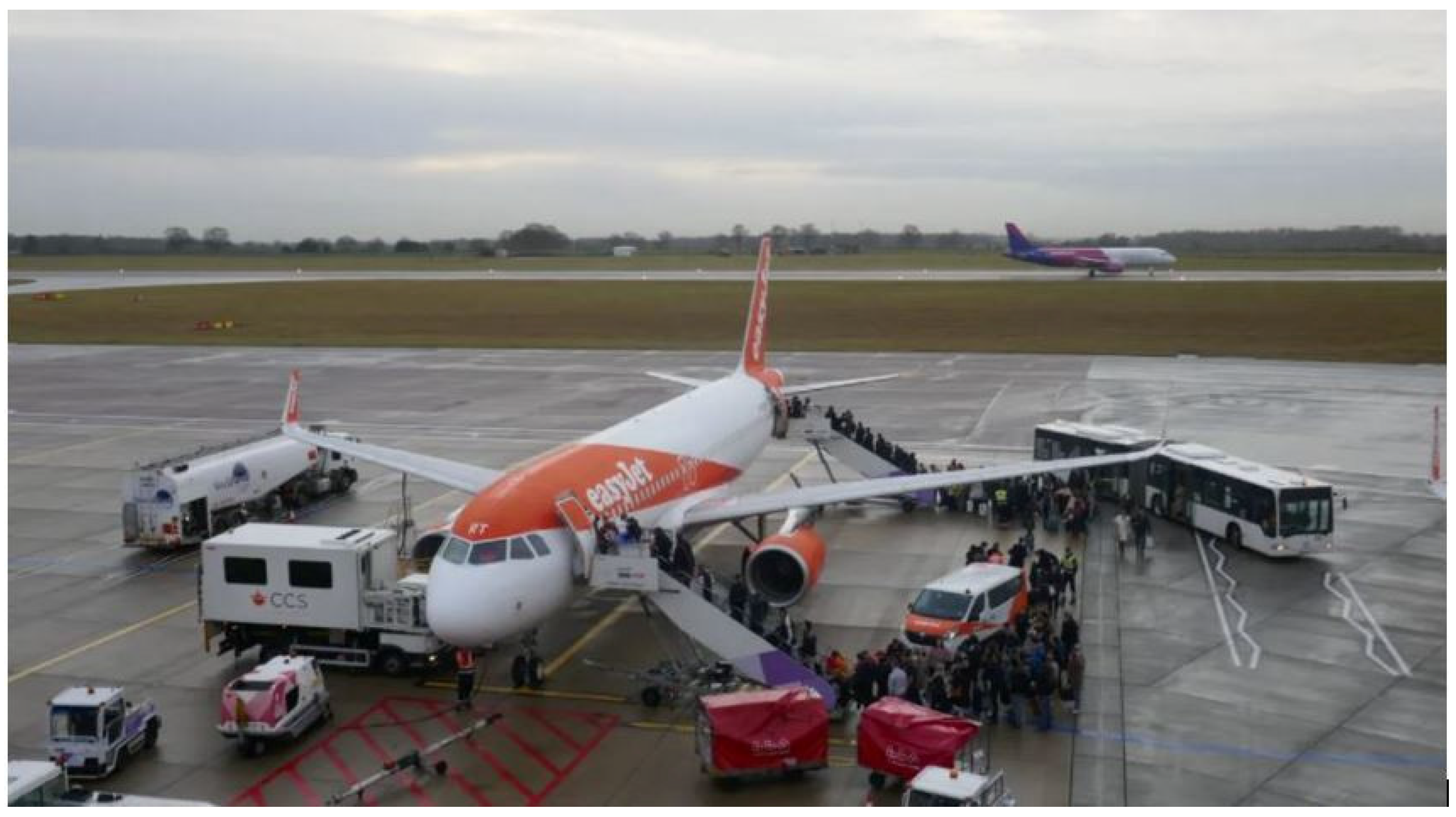
Ground support vehicles, such as galley service vehicles, baggage carts, bulk cargo loaders, jet bridges, lavatory service vehicles, cabin cleaning vehicles, potable water vehicles, and conditioned air vehicles, play a crucial role in the efficient operation of aircraft during a turnaround. Figure 2 visually represents these vehicles and their applications in aircraft servicing.

Energy Demand per GSE/Aircraft

Table 1. Energy consumption per GSE/aircraft.

Service	Company	Model	Power (kW)	Capacity (kWh)	Narrow Body Aircraft (min)	Energy Demand (kWh)	Small Body Aircraft (min)	Energy Demand kWh
Tractor	Trepel	Challenger 280e [46]	92	168	7	10.73	5	7.6
Ground power unit	ITW GSE	7400eGPU	90	160	40	60	40	60
Catering	Kamag	E-catering wiesel [47]	156	80	17	44.2	6	15.6
Transporter	Mulag	Pulsar 7E [48]	24	74.4	41	16.4	0	0
Baggage tractor	Mulag	Comet 6E [49]	40	124	45	30	27	18
Belt loader	Charlatte	CBL150E	1.3	28.8	41	0.88	23	0.49
Lavatory vehicle	Charlatte	CIT200E	30	40	14	7	0	0
Water truck	Charlatte	CWT300E [50]	30	40	14	7	0	0
	Airport with similar profile to under studied [51]					176.21		47.69

presents the estimated energy requirements for servicing small and narrow-body aircraft during turnaround operations based on the power and capacity of each EGSE vehicle, as provided by suppliers. The data takes into consideration the load and service time, as specified in references [40,44,45].

Table 2. Assumed daily energy demand from 40 flight data.

Scenarios	Narrow Body Aircraft (%)	Small Body Aircraft (%)	Energy Demand (kWh)
1	50	50	8956
2	30	70	6717
3	10	90	6054.2

summarises the total energy consumption for a hypothetical scenario of 40 flights with varying proportions of narrow-body and small-body aircrafts. These values will serve as the benchmark for measuring energy consumption in future phases of the study.

3. Methodology

3.1. Data Collection

The Cranfield Airport, a research platform for aviation technology development with world-class facilities such as the Digital Aviation Research Technology Centre [52], has a 1 MW solar farm on its premises. The farm has an installed ground array of 5858 square meters, comprising 3508 panels and 285 W PV modules. This array can generate an annual output of 1000 MWh of electricity. Historical data have been collected for both the PV output from the solar farm and the flight activities at a commercial airport with a similar profile to Cranfield Airport [51].

3.1.1. PV Output Data Collection

The solar farm energy record details the daily energy output supplied to the airport. The data were collected between 14 August 2018, and 1 April 2019, at 30 min intervals, resulting in 11,088 data points. After pre-processing, which involved using the Pandas date–time module to down-sample the data and increase the time granularity from hourly to daily, the number of data points was reduced to 231. In addition, the record contains photovoltaic (PV) output, irradiation, and temperature information.

3.1.2. Flight Data Collection

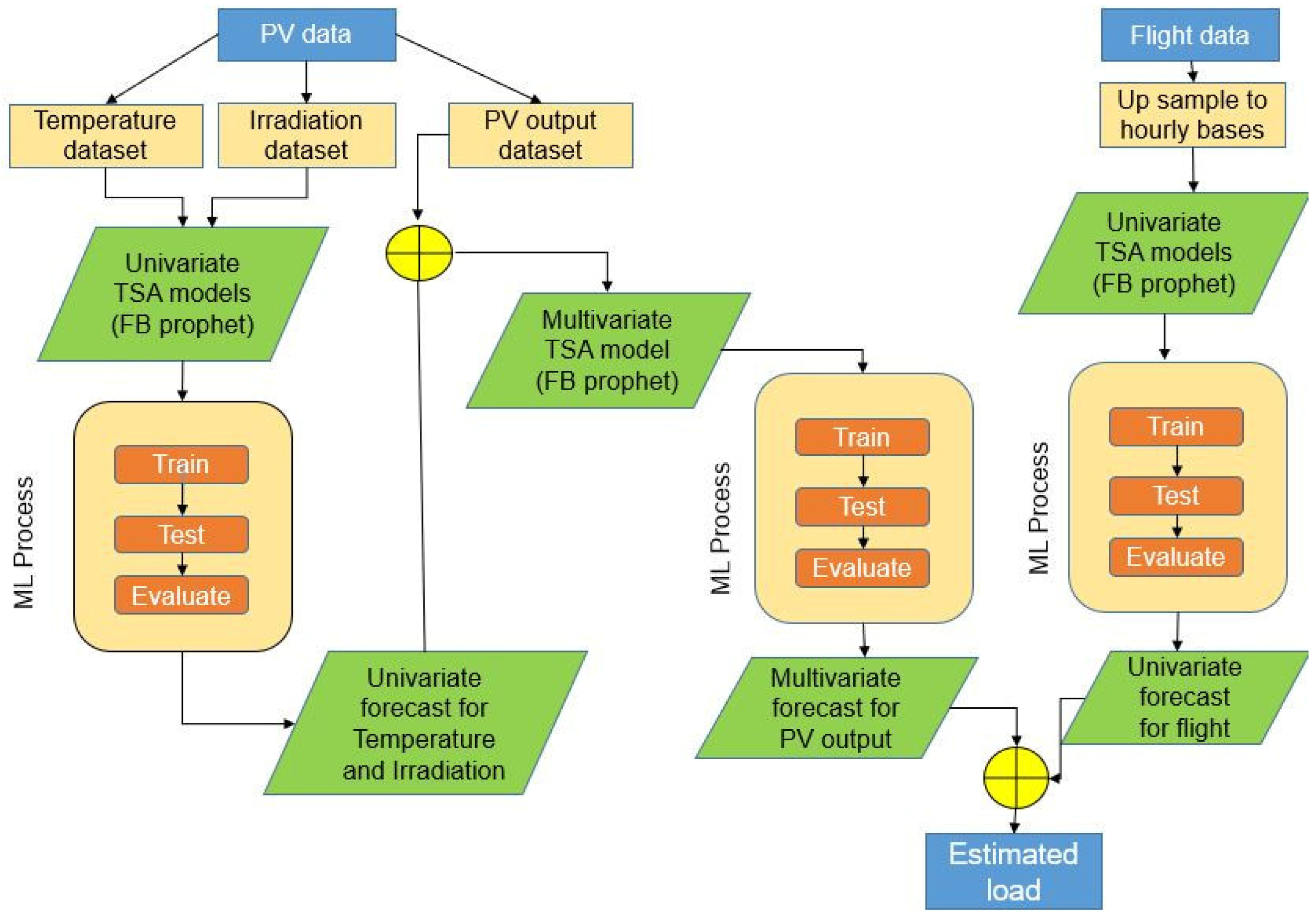
The flight data contains hourly records of the number of flights at the airport for 11 years, from 1 January 2011 to 1 December 2021. The dataset has been indexed according to the dates within the observation period, and the columns record the number of flights every hour of the day. This indexing resulted in a total of 3515 observations. The total number of flights per day has been calculated by taking a row-wise sum of the number of flights per hour, and was stored in a new variable, “flight total”. The flowchart of the modelling steps for the Facebook Prophet and VARIMA evaluation algorithm is shown in Figure 3.

3.2. Forecasting Method

Considering the multiple variables in the PV dataset that demonstrate potential causal relationships, as established by the Granger causality test, the vector autoregression (VAR) model emerges as a more fitting choice for forecasting PV output than an ARIMA model [53]. Therefore, a comparative evaluation is conducted between the VARIMA model and Facebook Prophet to analyse and forecast future PV outputs and flights. This evaluation incorporates univariate and multivariate time series analysis (TSA) techniques while assessing key regression metrics.

3.2.1. The Vector Autoregressive Integrated Moving Average Times Series Forecasting Tool

VARIMA is an extension of the autoregressive integrated moving average (ARIMA) model, which is commonly used to analyse univariate time series data. However, when forecasting in situations where the influence of other variables is significant but not accounted for in the model, univariate time series analysis may yield less accurate predictions [54].

Multivariate time series analysis, such as VARIMA, addresses this limitation. VARIMA models consist of four components: vector autoregressive (VAR), vector moving average (VMA), vector autoregressive moving average (VARMA), and vector autoregressive integrated moving average (VARIMA) [55]. These components allow for the incorporation of additional variables, enabling a more comprehensive representation of the relationships and dynamics among the variables under consideration. In addition, by considering the interplay between multiple variables, VARIMA models are better equipped to produce more representative and accurate forecasts. The mathematical formula for the VARIMA model is as shown in Equation (1) [56].

$$Y_t={\varnothing }_1{Y}_{t-1}+{\varnothing }_2{Y}_{t-2}+\dots .+{\varnothing }_p{Y}_{t-n}+{\in }_t$$

(1)

where Y_t is the observation, which is the linear combination of the values of the previous observation and the weight of each observation, which is adjusted to match the data. ${\varnothing }_i$ is the weight of each observation and ${\in }_t$ is the error vector.

3.2.2. Facebook’s Prophet Time Series Forecasting Tool

The Prophet algorithm is a time series model with inbuilt adjustable parameters that can suit the peculiarities of regular time series data, especially business time series. It is an open-source programme created by Facebook’s data science team for forecasting time series data that can fit nonlinear patterns with yearly, monthly, and daily seasonality and holiday effects, based on an additive model [26,36]. It excels in handling time series data with strong seasonal variation and historical data seasons. Compared to other predictive models, Prophet handles missing data, trends that shift over time, and outliers with remarkable efficiency. According to [57], FB Prophet has outperformed other methods in producing reliable forecasts within Facebook. In this paper, Prophet was utilized to model energy demand forecasts for ground movement operations at an airport, producing daily, weekly, and monthly forecasts. It operates on a decomposable time series model composed of three main components: trend, seasonality, and holidays. These components are combined in the following equation [58]:

$$y_t=g\left(t\right)+s\left(t\right)+h\left(t\right)+ℇ\left(t\right)$$

(2)

where g(t) is the trend function which is used to model non-periodic changes in the value of time series, s(t) is used to model periodic changes (e.g., weekly and annual seasonal changes), and h(t) is used to model the effects of holiday breaks over a few days. The error term ℇ_t refers to any change in characteristics the model cannot accommodate.

We divide the data into separate training (60%) and testing (40%) datasets to begin the process. Subsequently, the machine learning algorithm is applied to the training dataset, generating a prediction model. Finally, we assess the model’s performance by employing (10%) of the test dataset.

The data are processed using the Python data analysis library, Pandas, which can handle CSV, TSV, and SQL databases [37]. Once the data are loaded, Pandas creates a table-like structure, called a data frame, similar to a Microsoft Excel table. Next, Matplotlib is used to fit the individual forecasts from the FB Prophet to the needs of the operators. Finally, the Pandas library loads the CSV data into Matplotlib and designates the columns as “ds” and “y” as appropriate.

3.3. Forecast Accuracy Metrics

The forecast accuracy of univariate and multivariate time series models of the VARIMA and FB Prophet has been evaluated and compared using four essential measures. The models’ predictive ability is determined by aggregating the magnitude of forecast errors over time. The mean absolute error (MAE) represents the average difference between the predicted and actual observed values [59].

$$\mathrm{MAE}=\frac{1}{N}{\displaystyle \sum }_{I=1}^N\left|\left(P_{ft}-P_{mt}\right)\right|$$

(3)

The mean absolute percentage error (MAPE) is a widely used metric to evaluate the average percentage difference between the predicted and actual values [60]. It is particularly valuable in comparing forecast performance across diverse data sets due to its scale-independent nature. The MAPE can be expressed as follows [61]:

$$\mathrm{MAPE}=\frac{1}{n}\times {\displaystyle \sum }_{t=1}^n\left|\frac{P_{ft}-P_{mt}}{P_{ft}}\right|$$

(4)

The mean absolute percentage error (MAPE) has a limitation in that it penalizes positive errors more severely than negative errors. This can lead to issues when observations in the training set are close to zero or negative. To overcome this asymmetry in MAPE, and provide a more balanced assessment of errors, a symmetric mean absolute percentage error (SMAPE) has been introduced [62]. SMAPE is calculated as the average of all forecasts for a given horizon and has gained popularity in the machine learning community due to its desirable characteristics [63,64]. The SMAPE measures the average percentage deviation between the predicted and actual values, accounting for both underestimation and overestimation errors.

$$\mathrm{SMAPE}=\frac{1}{n}\times {\displaystyle \sum }_{t=1}^n\frac{\left|P_{ft}-P_{mt}\right|}{P_{ft}+P_{mt}}$$

(5)

The median absolute percentage error (MdAPE) is a measure of forecast accuracy that is calculated by arranging the absolute percentage error (APE) values in ascending order, then determining the middle value. If the number of values is even, the average of the two middle values is used.

$$\mathrm{MdAPE} =median\left(\frac{P_{ft}-P_{mt}}{P_{ft}}\right)$$

(6)

where $P_{mt}$ is the measured value, $P_{ft}$ is the value estimated by the forecasting model, and n is the size of the sample.

4. Results and Discussion

4.1. Exploratory Data Analysis (EDA) on PV Output Variables

4.1.1. Irradiation

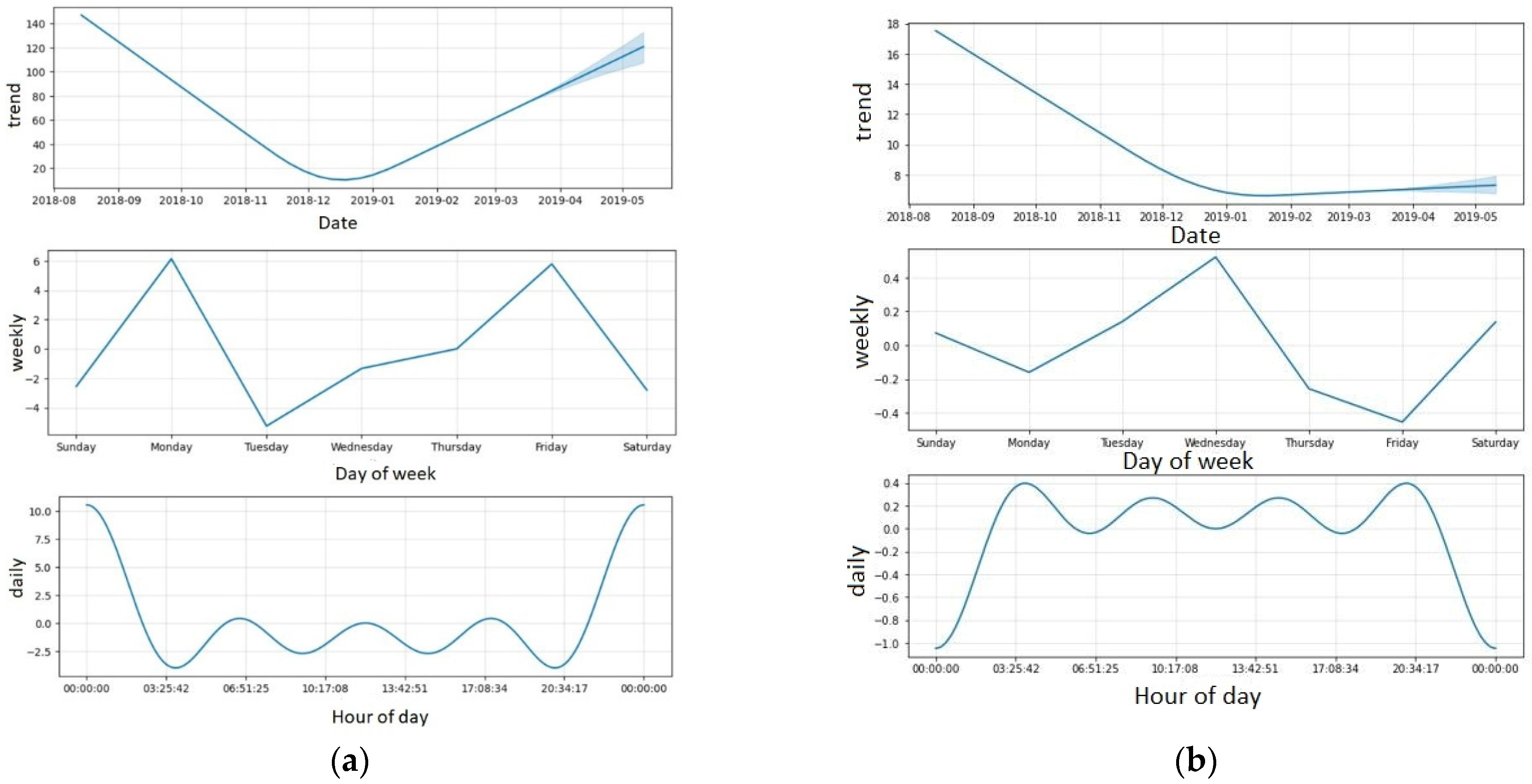
Irradiation is one of the two exploratory variables from the PV output dataset, defined as a numerical variable. Zero irradiations account for 50% of the variable, which explains the daily seasonality in the time series, stretching between evenings and early hours of the morning, when there is a scarcity of sunlight. The components graph Figure 4a shows a constant decrease in irradiation, with a trough in December 2019. This is followed by a steady rise in January 2019 throughout the observation period.

4.1.2. Temperature

Temperature is the second explanatory variable in the PV output dataset. Negative values account for 2.7% of the variable, corresponding to periods of temperature decreases. The components plot Figure 4b displays a clear trend of declining temperature over time.

4.1.3. PV Output

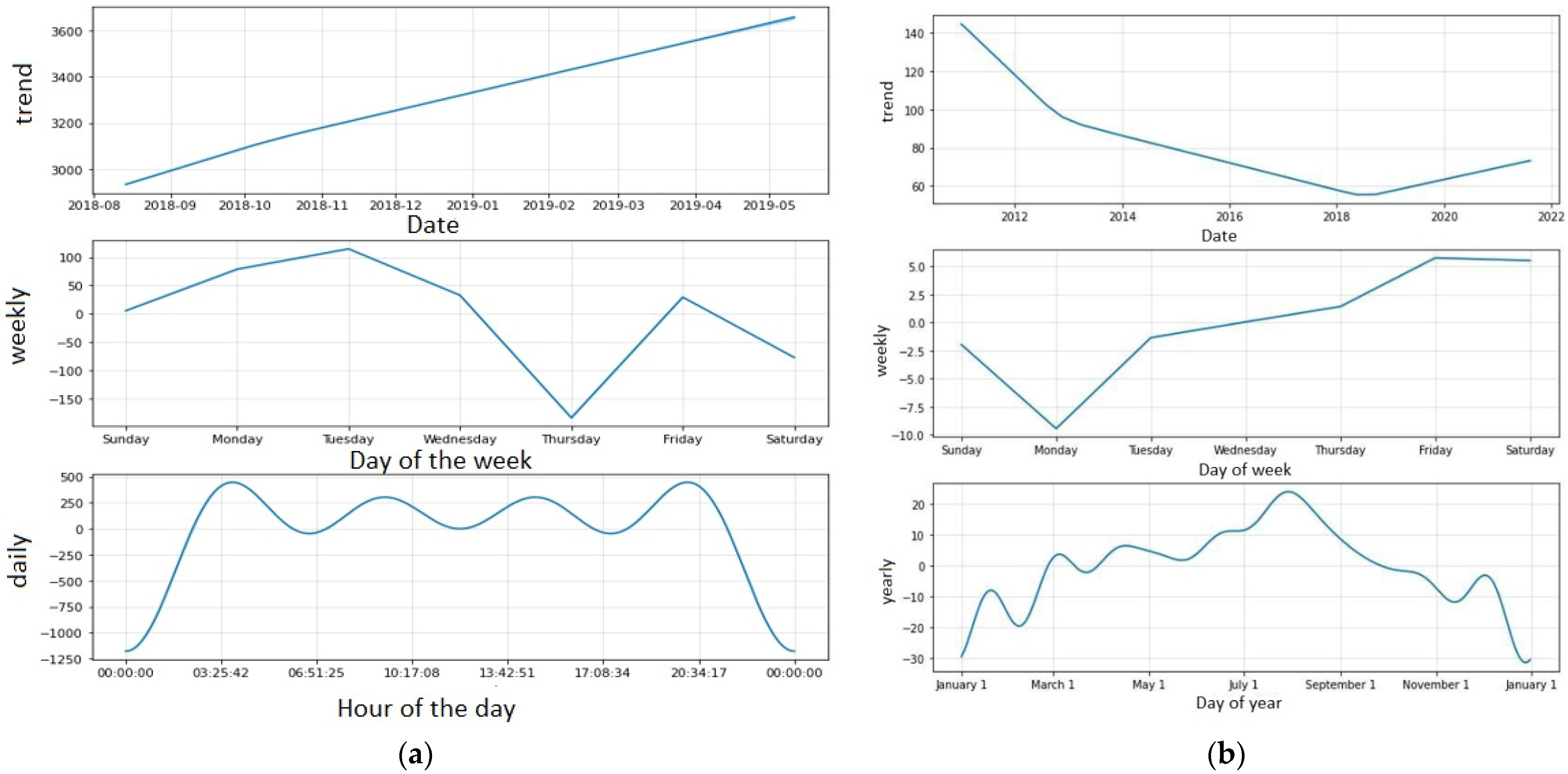
PV output is the target variable in the PV output dataset, which is a numerical variable. Zeros account for 55.1% of the variable. This value is due to periods of poor irradiation, which can be seen in the component plot Figure 5a between PV output and irradiation. This also accounts for the seasonality in the PV time series graph. The trend in the components plot shows a steady rise in PV output, a weekly peak on Tuesdays, and a trough on Thursdays.

4.2. EDA on Flight Data

The components plot in Figure 5b reveals a continuous decline in the number of flights from 2012 to 2018, followed by a steady rise from 2018 to 2022. The weekly number of flights declines between Sunday and Monday; there are fewer flights every week, gradually increasing until the following Sunday.

4.3. Forecast Results for Univariate and Multivariate Models on PV Output Data

Irradiation recorded at the ASPV within the observation period ranged between 345 and 10,496, with a mean value of 3478.56. The data show a consistent correlation between actual and forecasted irradiation within the forecast horizon, as depicted in the graph. Based on the evaluation metric for irradiation forecasting, the VARIMA and FB prophet models’ performance is as follows: The MAE for irradiation is 50.32, corresponding to an average difference of 0.56% MAPE between the predicted and actual values. The temperature ranged between −0.88 and 19.99 °C, with a mean of 8.96. The downward trend in temperature, as shown in Figure 4a, reflecting a steady decrease over the forecast horizon, aligns with the data observed during the period. The MAE for temperature was 7.20, corresponding to an average difference of 0.90% MAPE. The PV output values ranged from 0 to 5928.69, with a mean value of 2136.84. The forecast in Figure 5a shows consistency within the forecast horizon. The MAE for PV output was 1114.94, corresponding to an average difference of 0.58% MAPE between the predicted and actual values. The comparison of the performance metrics for the VARIMA and FB prophets is illustrated in

Table 3. Univariate models performance metrics for PV data variables.

Variable	MAE	MAPE	MdAPE	SMAPE
Irradiation
FB Prophet	50.32	0.56	0.58	0.80
VARIMA	51.81	39.59	39.46	46.97
Temperature
FB Prophet	7.17	0.89	0.90	1.63
VARIMA	1.95	21.98	24.69	25.21

,

Table 4. Multivariate models performance metrics for PV data variables.

Variable	MAE	MAPE	MdAPE	SMAPE
PV Output
FB Prophet	1115.05	0.58	0.42	0.46
VARIMA	1439.95	inf	41.64	56.26

and

Table 5. Univariate models performance metrics for total flight.

Variable	MAE	MAPE	MdAPE	SMAPE
Total flight
Prophet	38.82	3.44	0.55	0.74
VARIMA	52.30	53.53	30.40	65.37

.

Based on Table 3, a MAPE value of 0.56% indicates an excellent prediction model performance, with the predicted values closely matching the actual values. However, the interpretation of the MAPE value can vary, depending on the specific application. In cases where the predicted irradiation values are used for critical decision-making in energy production and revenue generation, even a small error can have significant financial implications. Conversely, a 0.56% MAPE is considered acceptable for monitoring and optimization purposes. With a MdAPE of 0.58%, the predicted irradiation values are very close to the actual values on average, with a small percentage deviation. The SMAPE of 0.80% suggests that, on average, the predicted irradiation values deviate from the actual values by only 0.80% in either direction. This low SMAPE value and MdAPE values signify a well-performing prediction model that provides accurate and consistent irradiation predictions with minimal deviation. It contributes to the effective operation and optimization of the solar PV system. A MAPE of 0.89% between the predicted and actual temperature values demonstrates a high level of accuracy in the prediction model; this value implies that the predicted temperature values deviate from the actual values by only 0.89% on average.

Accurate temperature predictions are crucial for a solar PV system, as they enable reliable estimation of temperature conditions that impact system performance and efficiency. They assist in assessing energy generation, identifying potential issues, and optimizing system operation. The low MAPE values indicate the prediction model’s effectiveness in providing accurate temperature forecasts, facilitating informed decision-making, maintenance planning, cooling strategies, and overall efficient management of the solar PV system.

Figure 6 and Figure 7 present the forecasts generated by the VARIMA and Prophet models, compared to the actual values of irradiation and temperature from the training set.

Figure 8 presents the forecasts generated by the VARIMA and Prophet models, compared to the actual values of PV output data from the training set.

4.4. Forecast Results for Univariate Model on Flight Data

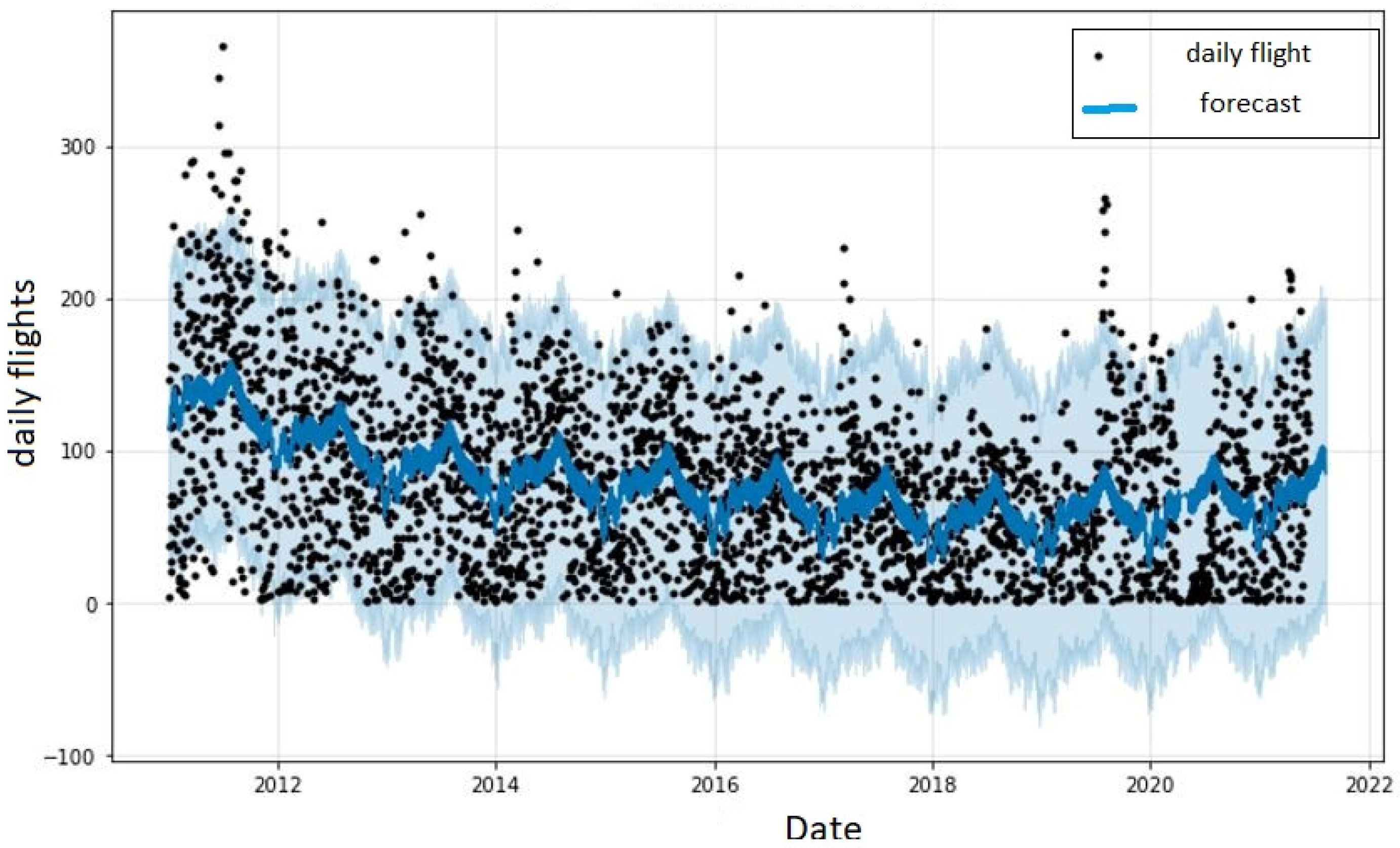
The number of flights recorded at the airport within the observation period ranged from 1 to 366, as shown from the data points in Figure 9 and Figure 10, with an average of 81 flights. Therefore, the MAE was calculated to be 38.87, corresponding to an average difference of 3.44% MAPE between the predicted and actual number of flights for the FB Prophet. Therefore, Figure 9 represents the observations and forecasts within the specified forecast horizon.

Table 5 provides insights into the accuracy of the predictive model by measuring the MAPE between the predicted and actual number of flights in an airport. A MAPE of 3.44% indicates that, on average, the predictive model’s forecasts deviate from the actual number of flights by 3.44%. This value quantifies the absolute percentage error in the predicted number of flights compared to the actual count.

Similarly, the SMAPE of 0.74% measures the accuracy of the prediction model about the flight schedule in the airport. This metric takes into account both underestimation and overestimation errors. For example, an SMAPE value of 0.74% means that, on average, the predicted flight schedule deviates from the actual schedule by only 0.74% in either direction. This high level of accuracy is crucial for accurately estimating flight timings, arrivals, and departures, providing reliable information for effective airport operations, resource allocation, and passenger flow management.

Figure 10 presents the forecasts generated by the VARIMA and Prophet models, compared to the actual values of flight data from the training set.

Upon analysing the Figure 6 and Figure 10, it becomes evident that the Prophet model exhibits a more accurate prediction pattern for irradiation, temperature, PV output, and flight data, effectively capturing the fluctuations in the test data. On the other hand, the VARIMA model’s predictions appear to follow a nearly linear trend [65]. These observations highlight the Prophet model’s superior performance in predicting actual values across all variables, underscoring the limitations of VARIMA in a stochastic environment.

4.5. Estimation of Energy Requirements for Ground Movement at Airports

To estimate the future cumulative available energy $E_T$, the actual ground movement energy demand at the airport has been subtracted from the forecasted PV output. The actual energy demand has been calculated by multiplying the energy demand of each EGSE by the predicted number of flights on specified future dates within the forecast horizon. Then, the actual value from the forecasted PV output is subtracted to obtain the available energy. The forecast horizon’s cumulative energy requirement can be calculated using Equation (7).

$$E_T={\displaystyle \sum }_{i=1}^n{\rho }_i-(u\times f_i)$$

(7)

where, $E_T$ is the cumulative energy requirement, n is the number of days within the forecast horizon, ${\rho }_i$ is the forecasted PV output, f is the forecasted number of flights, and u is the energy required by a single EGSE.

4.5.1. Scenario One

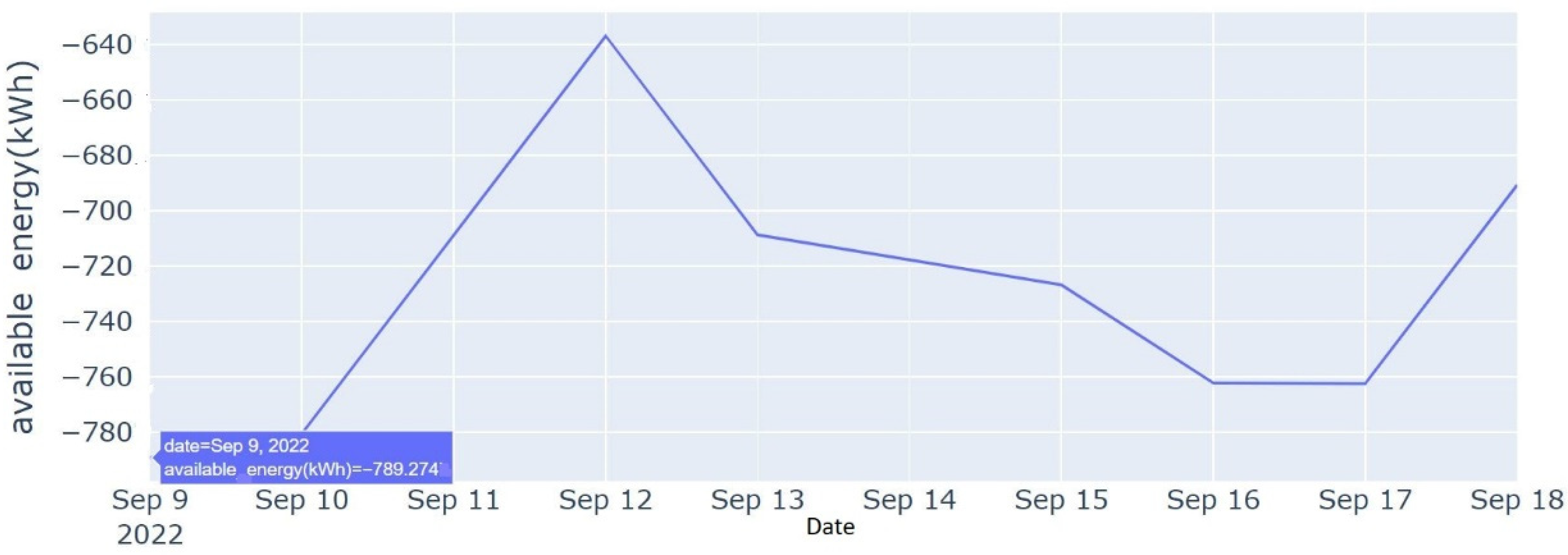
The worst case during this forecast horizon occurred on Friday (9 September 2022), when the energy deficit required to sustain ground movement operation was 789.27 kWh, as shown in Figure 11. On that day, the airport reaches the highest deficit between the EGSE energy demand and solar PV generation. That day corresponds to the airport’s peak traffic, as indicated in Figure 5b, which resulted in higher demand for EGSE and increased energy demand. On the following day of the week, net daily energy demand declined gradually. The day with the lowest energy deficit during the prediction horizon is Monday (12 September 2022), which corresponds with the beginning of the gradual airport traffic decline, as shown in Figure 5b.

4.5.2. Scenario Two

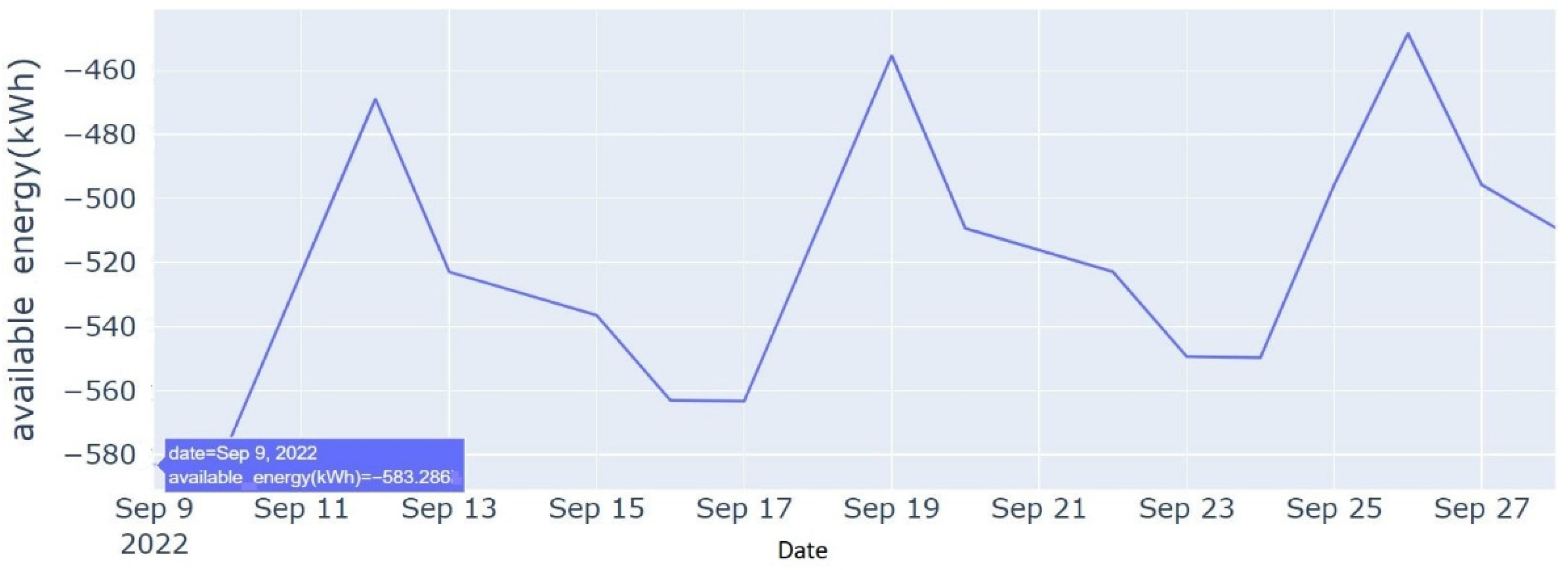
The minimum amount of energy required to ensure continuity of operations under this scenario is 583.286 kWh on the worst day within the forecasting horizon, as shown in Figure 12. Therefore, based on the forecasted PV generation and EGSE energy demand, September 16 and September 23 stand out as other critical days within the forecasting horizon.

4.5.3. Scenario Three

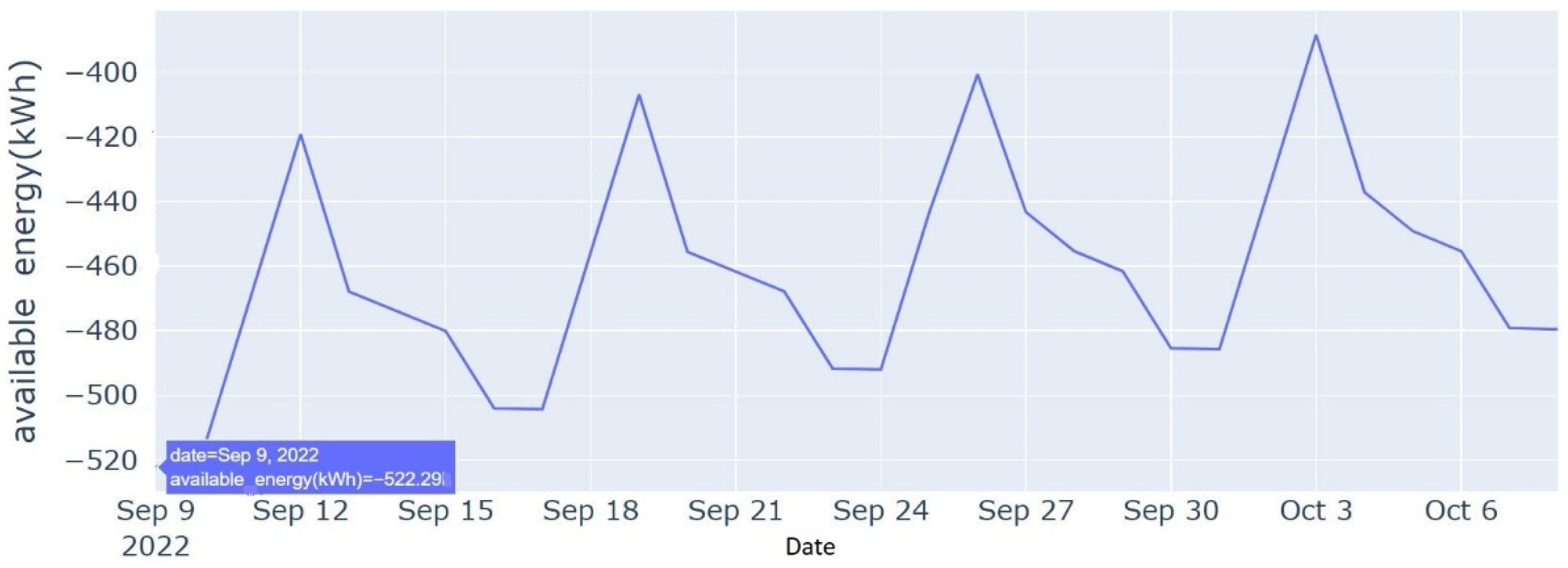
The minimum energy required on the worst day within the 30 days forecast horizon is 522.29 kWh, as shown in Figure 13. Other critical days within this forecasting horizon are September 16, September 23, September 30, and October 7. These specific dates experience the highest deficit between the energy demand of the Electrical Ground Support Equipment (EGSE) and the output of the photovoltaic (PV) system.

The models have been used to forecast the daily total number of flights and PV output and evaluate for accuracy using suitable metrics. In the univariate models on the PV output dataset for temperature and irradiation, MAPE ranged between 0.58 and 0.90, while SMAPE ranged between 0.83 and 1.64, accounting for a MAPE of 0.58 and SMAPE of 0.46 in the multivariate model forecasted PV output. The univariate model for total daily flights showed a MAPE of 3.44 and SMAPE of 0.74. Based on these error metrics and the forecast results, it can be stated that the models provide a useful estimate for predicting daily available energy.

The number of flights at any given moment is crucial in predicting ground movement. This number of flights has been used alongside estimated energy requirements by one EGSE to service a unit flight to estimate actual energy demand ahead. Hence, the total number of flights and energy generation has been treated as a time series problem. Univariate and multivariate time series models have been developed, using Facebook Prophet and VARIMA to forecast PV output at the ASPV and the total number of flights. The performance of the two models was compared, where FB Prophet outperforms the VARIMA based on the considered forecasting accuracy metrics. Therefore, the FB Prophet model is used to forecast the ground movement energy requirements in the airport. The three scenarios illustrate how the energy forecasting model allows operators to schedule the airport’s available energy sources economically and optimally. By merging decomposition, forecasts, and accuracy measures data into a single model, the model has streamlined the operators’ work and allowed direct output interpretation [27]. In general, it allows the operators to forecast the days with the highest energy demand, and more efficiently plan the scheduling of the energy sources. Finally, the fundamental pattern of the projection indicates that, on 9 September 2022, within the forecast horizon, the airport under examination has the most significant energy deficit.

5. Conclusions

Accurate energy projections and optimization play a critical role in the planning and allocation of resources in airports. By accurately forecasting future traffic and energy demand, airports can anticipate the needs of operators and make strategic adjustments to meet energy requirements. These adjustments include optimizing the utilization of the airport infrastructure to minimize energy consumption and reduce carbon emissions. The study presented in this paper compared the performance of two time series analysis models, namely Facebook Prophet and vector autoregressive integrated moving average (VARIMA), in predicting clean energy generation at airports. The study aimed to determine which model provided more accurate predictions by evaluating key performance metrics. The results indicate that the Facebook Prophet outperformed the VARIMA model, demonstrating its effectiveness in generating valuable predictions. These accurate predictions enable airport administrators to efficiently plan and manage energy usage, contributing to optimizing clean energy generation at airports.

Based on the Facebook Prophet model, the system effectively generates accurate energy predictions, providing practical guidance for planning increased electric load demand in the airside of future green airports. These efforts align with the zero-emission ground operation target outlined in the FlightPath 2050 policy.

In future studies, it would be beneficial to explore the implementation of additional renewable energy sources, such as vertical-axis wind turbines, to complement solar PV. Analysing the impact of these additional energy sources on the model results would provide a more comprehensive understanding of their contribution to energy generation. Overall, ongoing research and development in airport energy optimization will help airports achieve their sustainability goals, enhance operational efficiency, and contribute to a greener aviation industry.

References

1. Ferrulli, P. Green Airport Design Evaluation (GrADE)—Methods and Tools Improving Infrastructure Planning. Transp. Res. Procedia 2016, 14, 3781–3790. [Google Scholar] [CrossRef] [Green Version]
2. Nam, V.H. Green sustainable airports: The deployment of renewable energy at vietnam airports. Is that feasible ? J. Mech. Eng. Res. Dev. 2019, 42, 61–65. [Google Scholar] [CrossRef]
3. Acri, R.A.; Barone, S.; Cambula, P.; Cecchini, V.; Falvo, M.C.; Lepore, J.; Manganelli, M.; Santi, F. Forecast of the Demand for Electric Mobility for Rome–Fiumicino International Airport. Energies 2021, 14, 5251. [Google Scholar] [CrossRef]
4. Kang, M.; Bergέs, M.; Akinci, B. Forecasting Airport Building Electricity Demand on the Basis of Flight Schedule Information for Demand Response Applications. Transp. Res. Rec. J. Transp. Res. Board 2017, 2603, 29–38. [Google Scholar] [CrossRef]
5. Razak, F.A.; Shitan, M.; Hashim, A.H.; Abidin, I.Z. Load Forecasting Using Time Series Models. J. Kejuruter. 2009, 21, 53–62. [Google Scholar] [CrossRef]
6. Ahmad, T.; Zhang, D. A critical review of comparative global historical energy consumption and future demand: The story told so far. Energy Rep. 2020, 6, 1973–1991. [Google Scholar] [CrossRef]
7. Kuster, C.; Rezgui, Y.; Mourshed, M. Electrical load forecasting models: A critical systematic review. Sustain. Cities Soc. 2017, 35, 257–270. [Google Scholar] [CrossRef]
8. Patel, R.; Patel, M.; Patel, R.; Patel, M.R.; Patel, R.V. A Review: Introduction and Understanding of Load Forecasting 4 Publications 4 Citations See Profile a Review: Introduction and Understanding of Load Forecasting. June 2019. Available online: https://www.researchgate.net/publication/334108261 (accessed on 26 June 2022).
9. Debnath, K.B.; Mourshed, M. Forecasting methods in energy planning models. Renew. Sustain. Energy Rev. 2018, 88, 297–325. [Google Scholar] [CrossRef] [Green Version]
10. Grubb, M.; Edmonds, J.; Brink, P.; Morrison, M. The Costs of Limiting Fossil-Fuel CO2 Emis-Sions: A Survey and Analysis. Annu. Rev. Energy. Environ. 1993, 18, 397–478. [Google Scholar] [CrossRef]
11. Suganthi, L.; Samuel, A.A. Energy models for demand forecasting—A review. Renew. Sustain. Energy Rev. 2012, 16, 1223–1240. [Google Scholar] [CrossRef]
12. Pao, H. Forecasting energy consumption in Taiwan using hybrid nonlinear models. Energy 2009, 34, 1438–1446. [Google Scholar] [CrossRef]
13. Zhang, G.; Patuwo, B.E.; Hu, M.Y. Forecasting with artificial neural networks: The state of the art. Int. J. Forecast. 1998, 14, 35–62. [Google Scholar] [CrossRef]
14. Iwabuchi, K.; Kato, K.; Watari, D.; Taniguchi, I.; Catthoor, F.; Shirazi, E.; Onoye, T. Flexible electricity price forecasting by switching mother wavelets based on wavelet transform and Long Short-Term Memory. Energy AI 2022, 10, 100192. [Google Scholar] [CrossRef]
15. Shen, X.; Ou, L.; Chen, X.; Zhang, X.; Tan, X. The Application of the Grey Disaster Model to Forecast Epidemic Peaks of Typhoid and Paratyphoid Fever in China. PLoS ONE 2013, 8, e60601. [Google Scholar] [CrossRef] [Green Version]
16. Forouzanfar, M.; Doustmohammadi, A.; Menhaj, M.B.; Hasanzadeh, S. Modeling and estimation of the natural gas consumption for residential and commercial sectors in Iran. Appl. Energy 2010, 87, 268–274. [Google Scholar] [CrossRef]
17. Fan, T.-F.; Liau, C.-J.; Liu, D.-R. Rough Sets, Fuzzy Sets, Data Mining and Granular Computing; Springer: Berlin/Heidelberg, Germany, 2015. [Google Scholar]
18. Li, D.-C.; Chang, C.-J.; Chen, C.-C.; Chen, W.-C. Forecasting short-term electricity consumption using the adaptive grey-based approach—An Asian case. Omega 2012, 40, 767–773. [Google Scholar] [CrossRef]
19. Arslan, S. A hybrid forecasting model using LSTM and Prophet for energy consumption with decomposition of time series data. PeerJ Comput. Sci. 2022, 8, e1001. [Google Scholar] [CrossRef]
20. Keith, J.A.; Vassilev-Galindo, V.; Cheng, B.; Chmiela, S.; Gastegger, M.; Müller, K.-R.; Tkatchenko, A. Combining Machine Learning and Computational Chemistry for Predictive Insights Into Chemical Systems. Chem. Rev. 2021, 121, 9816–9872. [Google Scholar] [CrossRef]
21. Kumar, S.; Viral, R.; Deep, V.; Sharma, P.; Kumar, M.; Mahmud, M.; Stephan, T. Forecasting major impacts of COVID-19 pandemic on country-driven sectors: Challenges, lessons, and future roadmap. Pers. Ubiquitous Comput. 2021, 27, 807–830. [Google Scholar] [CrossRef] [PubMed]
22. Slater, L.J.; Arnal, L.; Boucher, M.-A.; Chang, A.Y.-Y.; Moulds, S.; Murphy, C.; Nearing, G.; Shalev, G.; Shen, C.; Speight, L.; et al. Hybrid forecasting: Using statistics and machine learning to integrate predictions from dynamical models. Hydrol. Earth Syst. Sci. Discuss. 2022, 1–35. [Google Scholar] [CrossRef]
23. Chujai, P.; Kerdprasop, N.; Kerdprasop, K. Time series analysis of household electric consumption with ARIMA and ARMA models. Lect. Notes Eng. Comput. Sci. 2013, 2202, 295–300. [Google Scholar]
24. Buhl, J.; Liedtke, C.; Schuster, S.; Bienge, K. Predicting the Material Footprint in Germany between 2015 and 2020 via Seasonally Decomposed Autoregressive and Exponential Smoothing Algorithms. Resources 2020, 9, 125. [Google Scholar] [CrossRef]
25. Liu, Y.; Roberts, M.C.; Sioshansi, R. A vector autoregression weather model for electricity supply and demand modeling. J. Mod. Power Syst. Clean Energy 2018, 6, 763–776. [Google Scholar] [CrossRef] [Green Version]
26. Song, X.; Liu, Y.; Xue, L.; Wang, J.; Zhang, J.; Wang, J.; Jiang, L.; Cheng, Z. Time-series well performance prediction based on Long Short-Term Memory (LSTM) neural network model. J. Pet. Sci. Eng. 2019, 186, 106682. [Google Scholar] [CrossRef]
27. Ma, Q.; Bi, J.; Sai, Q.; Li, Z. Research on Prediction of Checked baggage Departed from Airport Terminal Based on Time Series Analysis. In Proceedings of the 2021 7th Annual International Conference on Network and Information Systems for Computers (ICNISC), Guiyang, China, 23–25 July 2021; pp. 264–269. [Google Scholar] [CrossRef]
28. Wesonga, R.; Nabugoomu, F.; Ababneh, F.; Owino, A. Simulation of time series wind speed at an international airport. Simulation 2019, 95, 171–184. [Google Scholar] [CrossRef]
29. Miao, J. The Energy Consumption Forecasting in China Based on ARIMA Model. In Proceedings of the 2015 International Conference on Materials Engineering and Information Technology Applications, Guilin, China, 30–31 August 2015; pp. 192–196. [Google Scholar] [CrossRef] [Green Version]
30. Chen, B.; Zhao, X.; Wu, J. Evaluating Prediction Models for Airport Passenger Throughput Using a Hybrid Method. Appl. Sci. 2023, 13, 2384. [Google Scholar] [CrossRef]
31. Peng, Y.; Liu, H.; Li, X.; Huang, J.; Wang, W. Machine learning method for energy consumption prediction of ships in port considering green ports. J. Clean. Prod. 2020, 264, 121564. [Google Scholar] [CrossRef]
32. Azad, A.S.; Sokkalingam, R.; Daud, H.; Adhikary, S.K.; Khurshid, H.; Mazlan, S.N.A.; Rabbani, M.B.A. Water Level Prediction through Hybrid SARIMA and ANN Models Based on Time Series Analysis: Red Hills Reservoir Case Study. Sustainability 2022, 14, 1843. [Google Scholar] [CrossRef]
33. Oo, Z.Z.; Phyu, S. Time Series Prediction Based on Facebook Prophet: A Case Study, Temperature Forecasting in Myintkyina. Int. J. Appl. Math. Electron. Comput. 2020, 8, 263–267. [Google Scholar] [CrossRef]
34. Jha, B.K.; Pande, S. Time Series Forecasting Model for Supermarket Sales using FB-Prophet. In Proceedings of the 5th International Conference on Computing Methodologies and Communication, ICCMC 2021, Erode, India, 8–10 April 2021; pp. 547–554. [Google Scholar] [CrossRef]
35. Gupta, R.; Yadav, A.K.; Jha, S.; Pathak, P.K. Time Series Forecasting of Solar Power Generation Using Facebook Prophet and XG Boost. In Proceedings of the 2022 IEEE Delhi Section Conference (DELCON), New Delhi, India, 11–13 February 2022; pp. 1–5. [Google Scholar] [CrossRef]
36. Žunić, E.; Korjenić, K.; Hodžić, K.; Đonko, D. Application of Facebook’s Prophet Algorithm for Successful Sales Forecasting Based on Real-world Data. Int. J. Comput. Sci. Inf. Technol. 2020, 12, 23–36. [Google Scholar] [CrossRef]
37. Navratil, M.; Kolkova, A. Decomposition and Forecasting Time Series in the Business Economy Using Prophet Forecasting Model. Cent. Eur. Bus. Rev. 2019, 8, 26–39. [Google Scholar] [CrossRef] [Green Version]
38. Liu, Y.; Wu, J.; Tang, J.; Wang, W.; Wang, X. Scheduling optimisation of multi-type special vehicles in an airport. Transp. B Transp. Dyn. 2021, 10, 954–970. [Google Scholar] [CrossRef]
39. Tang, H.; Zhang, Y. Reducing Airport Pollution and Consequent Health Impacts to Local Community; U.S. Department of Transportation: Washington, DC, USA, 2018.
40. ACI EUROPE. Airport Carbon Accreditation. Available online: https://www.airportcarbonaccreditation.org/airport/4-levels-of-accreditation/optimisation.html (accessed on 3 May 2022).
41. Gulan, K.; Cotilla-Sanchez, E.; Cao, Y. Charging Analysis of Ground Support Vehicles in an Electrified Airport. In Proceedings of the 2019 IEEE Transportation Electrification Conference and Expo (ITEC), Detroit, MI, USA, 19–21 June 2019; pp. 1–6. [Google Scholar] [CrossRef]
42. Sari, M.; Mohamed, W.M.W.; Jalil, S.A. The Optimization Using Electric Ground Support Equipment in Aviation Industry. Int. J. Energy Econ. Policy 2022, 12, 401–406. [Google Scholar] [CrossRef]
43. Alruwaili, M.; Cipcigan, L. Airport Electrified Ground Support Equipment for Providing Ancillary Services to the Grid. SSRN Electron. J. 2022, 211, 108242. [Google Scholar] [CrossRef]
44. Fleuti, E. Aircraft Ground Handling Emissions Methodology and Emission Factors Zurich Airport. 2014. Available online: https://nap.nationalacademies.org/catalog/25233/microgrids-and-their-application-for-airports-and-public-transit (accessed on 19 October 2022).
45. National Academies of Sciences, Engineering, and Medicine. Improving Ground Support Equipment Operational Data for Airport Emissions Modeling; Transportation Research Board: Washington, DC, USA, 2015. [Google Scholar]
46. Challenger. Product Overview. 2013. Trepel Airport Equipment. Available online: https://trepel.com/products/aircraft-tractors/challenger-280e/ (accessed on 27 May 2023).
47. Kamag Presents Electric Catering Vehicle for All Aircrafts. 2019. Available online: https://www.electrive.com/2019/10/02/kamag-presents-electric-catering-vehicle-for-all-aircrafts/ (accessed on 27 May 2023).
48. Mulag. Pulsar 7E. Available online: https://www.mulag.de/en/ground-support-equipment/products/container-transporters/pulsar-7e/ (accessed on 27 May 2023).
49. Mulag. Comet 6E. Available online: https://www.mulag.de/en/ground-support-equipment/products/towing-tractors/comet-6e/ (accessed on 27 May 2023).
50. Charlatte. CWT300E. Available online: https://charlatteamerica.com/images/uploads/general/cwt300e.pdf (accessed on 28 May 2023).
51. Zhangjiajie Travel Guide. Zhangjiajie Hehua International Airport. Available online: https://www.zjjhhjc.com/pages_54/ (accessed on 18 September 2021).
52. Digital Aviation Research Technology Center (DARTeC). Available online: https://www.cranfield.ac.uk/centres/digital-aviation-research-and-technology-centre (accessed on 21 July 2021).
53. Yii, K.-J.; Geetha, C. The Nexus between Technology Innovation and CO2 Emissions in Malaysia: Evidence from Granger Causality Test. Energy Procedia 2017, 105, 3118–3124. [Google Scholar] [CrossRef]
54. Lusia, D.A.; Ambarwati, A. Multivariate Forecasting Using Hybrid VARIMA Neural Network in JCI Case. In Proceedings of the 2018 International Symposium on Advanced Intelligent Informatics (SAIN), Yogyakarta, Indonesia, 29–30 August 2018; pp. 11–14. [Google Scholar] [CrossRef]
55. Rusyana, A.; Tatsara, N.; Balqis, R.; Rahmi, S. Application of Clustering and VARIMA for Rainfall Prediction. IOP Conf. Ser. Mater. Sci. Eng. 2020, 796, 012063. [Google Scholar] [CrossRef]
56. Rusyana, A.; Rahmati, L.; Nurhasanah, N. Forecasting of Revenue, Number of Plane Movements and Number of Passenger Movements at Sultan Iskandar Muda International Airport Using the VARIMA Method. In Proceedings of the 1st International Conference on Statistics and Analytics, ICSA 2019, Bogor, Indonesia, 2–3 August 2019. [Google Scholar] [CrossRef]
57. Chakraborty, P.; Corici, M.; Magedanz, T. A comparative study for Time Series Forecasting within software 5G networks. In Proceedings of the 2020 14th International Conference on Signal Processing and Communication Systems (ICSPCS), Adelaide, Australia, 14–16 December 2020; pp. 1–7. [Google Scholar] [CrossRef]
58. Taylor, S.J.; Letham, B. Forecasting at Scale. Am. Stat. 2018, 72, 37–45. [Google Scholar] [CrossRef]
59. Qi, J.; Du, J.; Siniscalchi, S.M.; Ma, X.; Lee, C.-H. On Mean Absolute Error for Deep Neural Network Based Vector-to-Vector Regression. IEEE Signal Process. Lett. 2020, 27, 1485–1489. [Google Scholar] [CrossRef]
60. Hyndman, R.; Koehler, A.B. Another look at measures of forecast accuracy. Int. J. Forecast. 2006, 22, 679–688. [Google Scholar] [CrossRef] [Green Version]
61. Willmott, C.J.; Matsuura, K. Advantages of the mean absolute error (MAE) over the root mean square error (RMSE) in assessing average model performance. Clim. Res. 2005, 30, 79–82. [Google Scholar] [CrossRef]
62. Chicco, D.; Warrens, M.J.; Jurman, G. The coefficient of determination R-squared is more informative than SMAPE, MAE, MAPE, MSE and RMSE in regression analysis evaluation. PeerJ Comput. Sci. 2021, 7, e623. [Google Scholar] [CrossRef] [PubMed]
63. Maiseli, B.J. Optimum design of chamfer masks using symmetric mean absolute percentage error. EURASIP J. Image Video Process. 2019, 2019, 16–25. [Google Scholar] [CrossRef] [Green Version]
64. Hazarika, B.B.; Gupta, D.; Berlin, M. Modeling suspended sediment load in a river using extreme learning machine and twin support vector regression with wavelet conjunction. Environ. Earth Sci. 2020, 79, 1–15. [Google Scholar] [CrossRef]
65. García Nieto, P.J.; Sánchez Lasheras, F.; García-Gonzalo, E.; De Cos Juez, F.J. PM10 concentration forecasting in the metropolitan area of Oviedo (Northern Spain) using models based on SVM, MLP, VARMA and ARIMA: A case study. Sci. Total Environ. 2018, 621, 753–761. [Google Scholar] [CrossRef]
Figure 1. Structure of a basic model for forecasting or estimation [9].
Energies 16 05008 g001
Figure 2. Ground support equipment and vehicles servicing aircraft.
Energies 16 05008 g002
Figure 3. Flowchart of the modelling steps for the Prophet/VARIMA evaluation algorithm.
Energies 16 05008 g003
Figure 4. Component of the Prophet forecast for Cranfield Airport ASPV: (a) irradiation; (b) temperature.
Energies 16 05008 g004
Figure 5. Component of the Prophet forecast for Cranfield Airport: (a) PV output; (b) flight schedule.
Energies 16 05008 g005
Figure 6. Comparison of VARIMA and FB Prophet forecasts with actual irradiation value.
Energies 16 05008 g006
Figure 7. Comparison of VARIMA and FB Prophet forecasts with actual temperature value.
Energies 16 05008 g007
Figure 8. Comparison of VARIMA and FB Prophet forecasts with actual PV output.
Energies 16 05008 g008
Figure 9. Daily flight forecast in the airport.
Energies 16 05008 g009
Figure 10. Comparison of VARIMA and FB Prophet forecasts with actual flight data.
Energies 16 05008 g010
Figure 11. Daily optimized energy demand (10 day forecast horizon).
Energies 16 05008 g011
Figure 12. Daily optimized energy demand (20 day forecast horizon).
Energies 16 05008 g012
Figure 13. Daily optimized energy demand (30 day forecast horizon).
Energies 16 05008 g013