Article

Non-Intrusive Load Identification Method Based on KPCA-IGWO-RF

School of Electrical and Electronic Engineering, Hubei University of Technology, Wuhan 430068, China
*
Author to whom correspondence should be addressed.
Energies 2023, 16(12), 4805; https://doi.org/10.3390/en16124805
Submission received: 16 May 2023 / Revised: 13 June 2023 / Accepted: 17 June 2023 / Published: 19 June 2023

Abstract

:
Non-invasive load monitoring (NILM) represents a crucial technology in enabling smart electricity consumption. In response to the challenges posed by high feature redundancy, low identification accuracy, and the high computational costs associated with current load identification models, a novel load identification model based on kernel principal component analysis (KPCA) and random forest (RF) optimized by improved Grey Wolf Optimizer (IGWO) is proposed. Initially, 17 steady-state load characteristics were selected as discrimination indexes. KPCA was subsequently employed to reduce the dimension of the original data and diminish the correlation between the feature indicators. Then, the dimension reduction in load data was classified by RF. In order to improve the performance of the classifier, IGWO was used to optimize the parameters of the RF classifier. Finally, the proposed model was implemented to identify 25 load states consisting of seven devices. The experimental results demonstrate that the identification accuracy of this method is up to 96.8% and the Kappa coefficient is 0.9667.

1. Introduction

Power Internet of Things (PIoT) technology and smart meters are widely used in many fields, such as smart building controls [1], plug load automation [2], building energy assessment [3], household appliance power consumption [4], etc. These applications have led to the accumulation of massive amounts of energy data. These data provide powerful support for load monitoring, with potential benefits for both end-users and power supply departments. Specifically, load monitoring can enable users to gain detailed insights into the power consumption patterns of various household appliances during different time periods, thereby facilitating the development of energy-saving plans and reducing the overall electricity costs. Load monitoring techniques can be divided into intrusive load monitoring (ILM) and non-intrusive load monitoring (NILM). Through ILM approaches, it is possible to obtain high-resolution data [5]. However, ILM is a costly approach compared to NILM. NILM approaches do not require the installation of sensors on each appliance, which reduces the monitoring cost. NILM technology was initially proposed by Professor Hart [6] with the main aim of acquiring the working state information of each electrical appliance by analyzing the electric energy data of the user bus. After more than three decades of development, the research methods of NILM technology have become increasingly diverse and sophisticated. Kamat et al. [7] proposed a pattern recognition method based on fuzzy logic theory to analyze equipment energy consumption by calculating the transient power differences between device switching states. However, this method was limited to analyzing only two-state devices in the ON/OFF process and was not applicable to scenarios involving the frequent switching of the multi-state device. Bonfigli et al. [8] proposed a bivariate hidden Markov model that utilizes active power and reactive power for load decomposition, and verified its effectiveness in both noisy and de-noised environments. However, this method is not well suited for handling appliances with similar power characteristics. Wu et al. [9] proposed a load decomposition method combining adaptive density peak clustering and the hidden Markov model (DPC-FHMM). This method can automatically determine the working state information of electrical appliances and reduce the dependence on historical data. However, this algorithm only targets the active power load characteristic, and has limitations on the division of electrical appliances’ working state. Kosuke et al. [10] proposes a load decomposition method based on integer programming, which determines the types of connected appliances by analyzing changes in current waveforms. Although this method has good expandability, it requires a large amount of calculation. Hasan et al. [11] proposed a load identification model using the V-I trajectory, which was validated for its robustness and reliability on the REDD public dataset. Gillis et al. [12] proposed a method using wavelet design and Procrustes analysis to match the wavelet energy with the load for signal feature extraction, followed by building a semi-supervised machine learning model for load identification. However, the calculation model of this method is complex and greatly affected by noise. Huang et al. [13] proposed the use of fast Fourier transform (FFT) to process high-frequency current information from the REDD dataset, obtaining 1–16 harmonics. Principal component analysis (PCA) was then used to reduce the dimensionality of the harmonics, followed by the application of the LSTM-BP neural network for load identification. Fang et al. [14] proposed a load decomposition model based on feature multiplexing long- and short-memory network (M-LSTM). The method first utilizes an improved multi-scale fusion residual module to extract base load features, followed by using the LSTM cycle unit to extract time series information. Popescu et al. [15] established the suitability of the recursive graph analysis method for mining load characteristics. This method applies the nonlinear analysis of the current waveform to extract characteristics that can enhance the accuracy of load identification models. The experiments were conducted on common household appliances to verify the efficacy of the proposed method. Zhou et al. [16] proposed a method for electrical recognition by combining V-I trajectory features and current harmonic features through a binarization process to form a combination matrix, which was then input into a convolutional neural network (CNN). This approach improves the accuracy of electrical recognition by integrating both time-domain and frequency-domain features. Dufour et al. [17] utilized a low-frequency acquisition device to collect the active and reactive power datasets of household appliances, and constructed load identification models using support vector machine (SVM) to identify the operating states of heating equipment and water heaters. However, the input features of this model were limited, making it unsuitable for low-power and similar power devices, and it did not consider the combined operation of multiple loads.
In light of the prevailing issues of considerable feature redundancy, limited identification accuracy, and substantial computational costs observed in current load identification models, this paper introduces a method to address these challenges. Specifically, we leverage KPCA to reduce the dimensionality of steady-state load data. The resulting feature data are then used as input for an RF classifier, with the load status label serving as the output. The key parameters of the RF classifier are optimized using IGWO, and the proposed approach is validated using 25 load states involving seven different electrical appliances. The experimental results demonstrated the effectiveness of the proposed method in accurately identifying the load state, with potential applications for enhancing energy management practices and promoting more sustainable energy consumption habits.

2. Load Identification Model

2.1. Kernel Principal Component Analysis

KPCA is an enhanced version of principal component analysis (PCA) algorithm [18]. The central concept of KPCA involves the mapping of nonlinear data samples to a high-dimensional space using a kernel function, followed by dimensionality reduction using PCA. While there are several advanced dimensionality reduction approaches available [19,20] in the literature, KPCA dimensionality reduction has been chosen in this study mainly because of its special advantages in processing nonlinear data.
For the eigensample matrix X = x 1 , x 2 , , x n T , the number of samples is n, the dimension of each sample is m, and the nonlinear function φ is used to map the original sample from m dimension to d dimension space (d > m). The original matrix X is converted into the new matrix φ(X):
φ ( X ) = φ x 1 , φ x 2 , , φ x n
The covariance matrix C of φ(X):
C = 1 n i = 1 n φ x i φ x i T = 1 n φ ( X ) φ ( X ) T
According to the eigenequation λ V = C V , the eigenvalue λ of C and the corresponding eigenvector V are obtained, respectively. Since PCA does not consider the eigenvalue 0 in dimension reduction, only the non-0 eigenvalue is retained. Suppose that, when λ 0 , there exists a coefficient vector α = α 1 , α 2 , , α n T that the eigenvector V can be represented linearly as:
V = i = 1 n α i φ x i
Substitute Equation (3) into the characteristic equation of C, and multiply the matrix φ ( X ) T on both sides of the equation:
φ ( X ) T φ ( X ) φ ( X ) T φ ( X ) α = λ φ ( X ) T φ ( X ) α
A kernel matrix K = φ ( X ) T φ ( X ) is defined, any element in the matrix can be expressed as:
k i j = k x i , x j = φ x i T φ x j
Then, Equation (4) can be converted into:
K α = λ α
The eigenvalue of K and its corresponding eigenvector are obtained from Equation (6), and then the normalized eigenvector of C is obtained, and the KTH principal component of sample X is:
h k = v k φ ( x ) = i = 1 m α i k k x i , x j
According to the eigenvalue of the kernel matrix K, the contribution rate of each principal component is calculated, selecting the maximum t eigenvalues and corresponding eigenvector ri when the contribution rate reaches p (p is generally 85~95%):
λ 1 + λ 2 + + λ t λ 1 + λ 2 + + λ m p
The matrix after dimensionality reduction is:
Y = K T r = K T 1 λ 1 r 1 , 1 λ 2 r 2 1 λ t r t

2.2. Improved Grey Wolf Optimizer

Grey Wolf Optimizer (GWO) [21] draws inspiration from the social behavior of wolves in the wild, particularly their collective hunting strategies. By simulating this natural process, the GWO algorithm is designed to achieve the optimization objectives more effectively and efficiently. Mimicking the order of the pack class from highest to lowest, the algorithm defines the first three optimal solutions as α, β and δ, the rest of the solutions are defined as ω, and its mathematical model can be described as:
D = C X p ( t ) X ( t )
where t is the current iteration number, D is the distance between the wolf and its prey, X p ( t ) and X ( t ) are the position vectors of the prey and gray wolf, respectively, C = 2 · r 1 , A = 2 a · r 2 a , r 1 and r 2 are random numbers between 0 and 1, a decreases linearly from 2 to 0 as t increases.
After the hunting behavior begins, ω updates its position based on the position of α, β and δ:
D α = C 1 X α X
D β = C 2 X β X
D δ = C 3 X δ X
D α , D β , and D δ , respectively, represent the distance between α and ω, β and ω, and δ and ω, whilst C 1 , C 2 and C 3 are random vectors. X α , X β , and X δ are the position vectors of α, β, and δ, respectively, whilst the position update formula is:
X 1 = X a A 1 D α
X 2 = X β A 2 D β
X 3 = X δ A 3 D δ
X ( t + 1 ) = X 1 + X 2 + X 3 3
In practical applications, GWO has been observed to suffer from slow convergence and a tendency to become trapped in local optima. To address these limitations, an improved version of the algorithm known as Improved Grey Wolf Optimizer (IGWO) has been proposed, and the specific improvement strategies are as follows:
(1) Compared to traditional algorithms that use random initialization, generating initial populations using chaotic sequences can increase diversity and improve the global search ability of an optimization algorithm. While the logistic mapping method is commonly used for generating chaotic sequences, recent research [22] suggests that Tent mapping may offer better uniformity and faster iteration speeds. The Tent mapping iteration function can be expressed as follows:
X ( t + 1 ) = 2 X ( t ) , 0 X ( t ) 0.5 2 ( 1 X ( t ) ) , 0.5 X ( t ) 1
By mapping the sequence generated using the Tent mapping function to the value range required for optimization, a chaotic initialization sequence can be obtained. This approach leverages the highly irregular and unpredictable behavior of chaotic systems to generate a sequence of values that can help improve the diversity and effectiveness of optimization algorithms.
(2) The traditional algorithm employs a linear decrease in the convergence factor from 2 to 0, which may not reflect the nonlinear convergence process of the algorithm. To address this issue, we propose a novel convergence factor change function that utilizes the sine function, whose expression is:
a = 2 2 sin π 2 t t max 2
In the proposed convergence factor strategy, the algorithm can maintain a high convergence factor for a longer period during the early stage of the iteration, thereby enhancing its search efficiency and increasing the likelihood of capturing the potential optimal solutions. During the later stages of the iteration, the convergence factor decreases rapidly, allowing the algorithm to perform a local search near the optimal solution.
(3) The search strategy of GWO centers around the approach of all populations to the wolves at the decision-making level for capturing prey. Hence, the quality of these wolves will significantly impact the overall search effectiveness. To prevent the algorithm from converging to local optimal solutions, we introduce chaotic disturbance to the three wolves at the decision-making level. The following strategies are employed:
n e w X = η X t + ( 1 η ) X
where newX is the position of wolf after adding disturbance, Xt is a chaotic sequence obtained by Tent mapping, and X is the position of the individual whose disturbance is added. η is the disturbance factor. The change function of η is:
η = lg t + 9 t
where t is the number of iterations.

2.3. Random Forest

Random forest [23] is a widely used classifier that consists of multiple classification regression trees. Decision trees are effective in classification, but they tend to overfit when dealing with complex and heterogeneous data. To address this issue and improve the classification accuracy, ensemble learning techniques are often used to combine multiple classifiers. Ensemble learning can be categorized into two types: serial Boosting and parallel Bagging. The random forest algorithm belongs to the Bagging method. Its main idea is to create decision trees on multiple random subsets of the data, and then combine the prediction results of these decision trees through voting to obtain the final prediction result of the random forest. Each decision tree in the random forest is relatively independent, making it less likely to overfit the training data. Therefore, compared with a single decision tree, the random forest model has a stronger generalization ability and robustness.
In the RF algorithm, the two key parameters that can have a significant impact on the classification accuracy of the model are the maximum depth of the decision tree (dp) and the number of decision trees (es) [24]. To achieve the best identification effect of the RF model, the IGWO algorithm is utilized to optimize these parameters. By searching the parameter space with the IGWO algorithm, the optimal values of dp and es can be determined. The optimized RF model can then achieve better classification performance in identifying the load state of electrical appliances.

2.4. KPCA-IGWO-RF Load Identification Model Flow

In order to enhance the efficiency of load identification and reduce redundancy in the original feature data, we employed KPCA to reduce the dimensionality of the original load feature data and filter out noise. Next, the RF algorithm was utilized to classify and identify running loads. However, the selection of parameters has a significant impact on the identification accuracy of the RF model. Therefore, to achieve optimal results, we employed the IGWO algorithm to determine the optimal values for the dp and es parameters. Figure 1 displays the KPCA-IGWO-RF load identification model, based on the aforementioned approach.

3. Experimental Verification

3.1. Data Acquisition and Identification Feature Selection

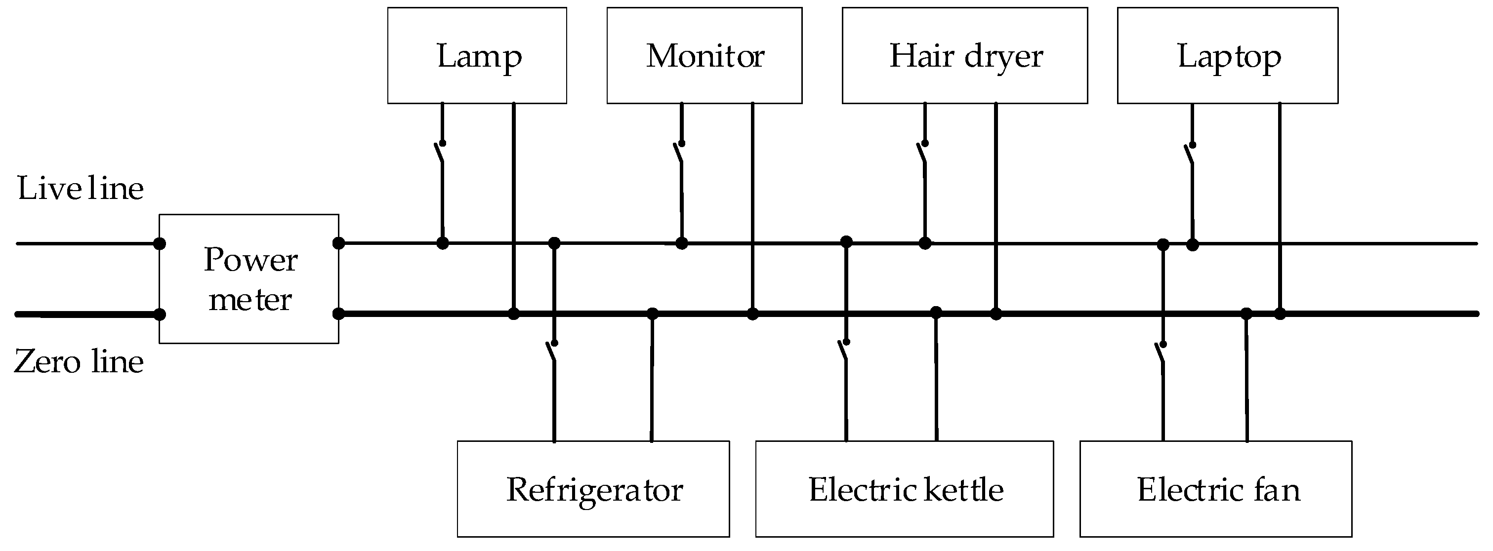
In the laboratory experiment, we selected seven common electrical appliances, namely the electric kettle, lamp, refrigerator, laptop, monitor, hair dryer, and electric fan, and connected them to the same bus. The steady-state characteristic data of the load were measured and collected using a power meter located at the entrance of the bus. The arrangement of the power meter and electrical appliances in the laboratory is depicted in Figure 2.
Among the seven electrical appliances in the laboratory, the monitor, electric kettle, and lamp are categorized as switch type devices. The hair dryer and electric fan belong to the limited multi-state load category. The hair dryer has three gears, while the electric fan has two gears. The refrigerator and laptop are classified as continuous change state type loads, where their power values fluctuate irregularly during operation. Additionally, the electric kettle is a pure resistance device with a power factor of 1, meaning that the active power and current exhibit the same trend, and no reactive power is generated. The motors contained in the refrigerators, hair dryers, and electric fans establish magnetic fields by inductance windings, which introduce a phase difference between current and voltage, resulting in the generation of reactive power. The switching power supplies used in laptops and monitors consume energy to control the switch during the conversion of electrical energy, producing reactive power. All lights in the laboratory belong to optical devices, which generate relatively low active power, reactive power, and current. Particularly, when multiple loads operate simultaneously, accurately identifying the load type solely based on the current and power characteristics can be challenging.
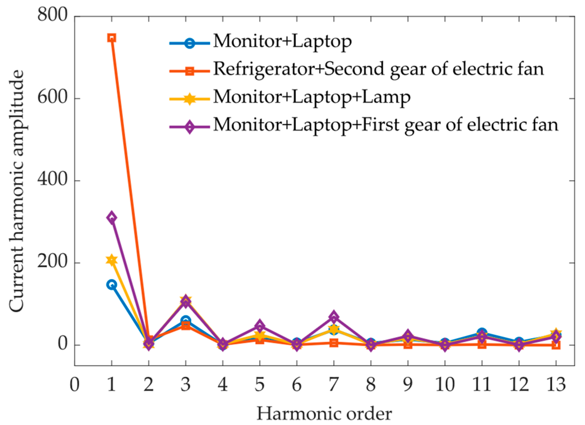
As a higher frequency and dimension frequency domain characteristic, harmonics can contain more load information. Figure 3 illustrates the current harmonic amplitude of a sampling point when some devices run individually, while Figure 4 shows the current harmonic amplitude of a sampling point when some electrical appliances are run in combination.
The amplitude of odd-order harmonics is typically larger than that of even harmonics generated by electrical appliances, and even harmonics are generally close to 0. However, experimental measurements revealed that, when the hair dryer is running in the second gear position or in combination with other equipment, the amplitude of even harmonics becomes larger. Figure 5 illustrates the harmonic amplitude of the hair dryer’s three gear positions.
It is evident from Figure 5 that even harmonics can provide valuable load information, and therefore can potentially impact the results of the load identification model. However, it can be challenging to avoid omitting relevant feature information when relying on subjective judgment to select a specific harmonic as the original feature. In order to address this issue, this study selects a comprehensive set of 17 steady-state load features as the original features of the identification model, including active power P, reactive power Q, effective value of current I, power factor λ, and the first to 13th current harmonic amplitudes (I(1)–I(13)).
To evaluate the efficacy of the proposed model, a total of 25 load states in combination with seven typical electrical appliances were randomly employed, where 10 of them were single load states. Specifically, the single load states comprised Monitor (L1), laptop (L2), hot water bottle (L3), table lamp (L3), refrigerator (L5), hair dryer first gear (L6), hair dryer second gear (L7), hair dryer third gear (L8), electric fan first gear (L9), and the electric fan second gear (L10). The labeling of each load state along with the corresponding electrical appliance is presented in Table 1.

3.2. Principal Component Extraction Based on KPCA

In this study, KPCA was employed to extract the features of the 17 load characteristic indicators. The eigenvalues of sample data were initially calculated, followed by determining the contribution rate of each eigenvalue corresponding to the eigenvector. The individual contribution rate and cumulative contribution rate of each principal component are graphically presented in Figure 6.
Based on Figure 6, the first five principal components contribute the most to the extracted features, with contribution rates of 39.45%, 21.43%, 14.37%, 11.63%, and 8.26%, respectively. The cumulative contribution rate of the first five principal components is 95.14%, which is more than 95%. In contrast, the last three principal components only have contribution rates of 2.36%, 0.85%, and 0.38%, respectively, resulting in a cumulative contribution rate of only 3.59%. Thus, it is concluded that the first five principal components are sufficient to represent all the feature information.

3.3. Load Identification Evaluation Index

The performance of the classifier needs specific performance indicators to be tested. We use accuracy and Kappa coefficient to evaluate the performance of the load identification model.
(1) For multi-classification problems, the calculation method of accuracy is:
  accuracy = N M
where N is the number of correctly classified data strips and M is the number of total test data strips.
(2) Kappa coefficient [25] is usually used for consistency verification and can measure classifier performance when the category distribution is unbalanced. The solution method of Kappa coefficient is:
Kappa = p 0 p c 1 p c
where p0 is the total classification accuracy, and it is assumed that the actual number of samples for each category is a1 and a2... ac, the number of samples for each type predicted by the classifier is b1, b2... bc, and the total number of samples is n; then, the solution method of pc is as follows:
  p c = a 1 × b 1 + a 2 × b 2 + a c × b c n × n
The value of the Kappa coefficient is between 0 and 1, and the larger the value, the better the classification performance of the classifier.

3.4. Test of KPCA-IGWO-RF Load Identification Model

Based on the corresponding relationships between the load and label, as determined in Table 1, a total of 2500 groups of steady-state characteristic data were collected, with 100 groups randomly measured for each label. The collected data were then divided into training and testing sets in a ratio of 7:3 for each label. The load identification model of KPCA-IGWO-RF was constructed using the first five principal components extracted from KPCA as inputs and load type labels as inputs. The specific steps of the model construction are outlined as follows:
(1) The initialization parameters of IGWO were set as follows: considering that the optimization targets are dp and es, the dimension of the solution is 2, the initial population size of wolves is set to 30, and the maximum number of iterations is set to 100. Furthermore, the error rate of the identification results was chosen as the fitness function.
(2) To optimize the RF model, the interval for dp optimization was set to [0, 50], and the interval for es optimization was set to [0, 300]. Additionally, the number of binary trees was set to 20, and the number of node partition sample classes was set to 15.
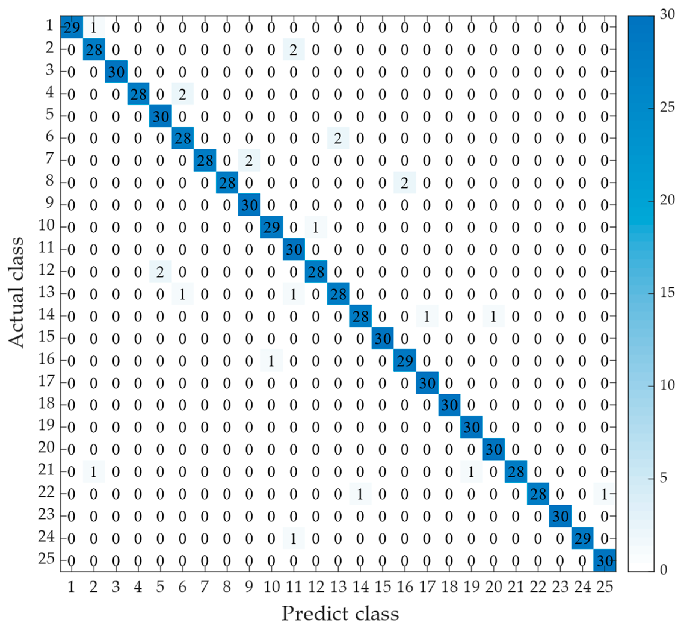
(3) The KPCA-IGWO-RF model was constructed using the MATLAB R2020a platform. After training with 1500 sets of data representing 25 types of load labels, simulation tests were performed on 750 sets of data to determine the accuracy of load identification. The classification performance of the KPCA-IGWO-RF model was evaluated through the generation of a confusion matrix, as depicted in Figure 7.
Based on the identification results obtained from our study, the KPCA-IGWO-RF model demonstrated a high level of accuracy in identifying load labels. Specifically, for one-load labels 1–10, the model exhibited an impressive identification accuracy of 96%. Similarly, for two-load labels 11–18, the model achieved a commendable identification accuracy of 97.0833%. For three load labels 19–25, the model’s identification accuracy was 97.6190%. Overall, the KPCA-IGWO-RF model displayed a robust identification performance, with an overall identification accuracy of 96% and a Kappa coefficient of 0.9667, which indicates a high degree of agreement between the model’s predictions and the actual observations.
(4) To further evaluate the effectiveness and reliability of the model, the RF model, KPCA-RF model, and KPCA-GWO-RF model were also compared, and the final experimental results are presented in Table 2.
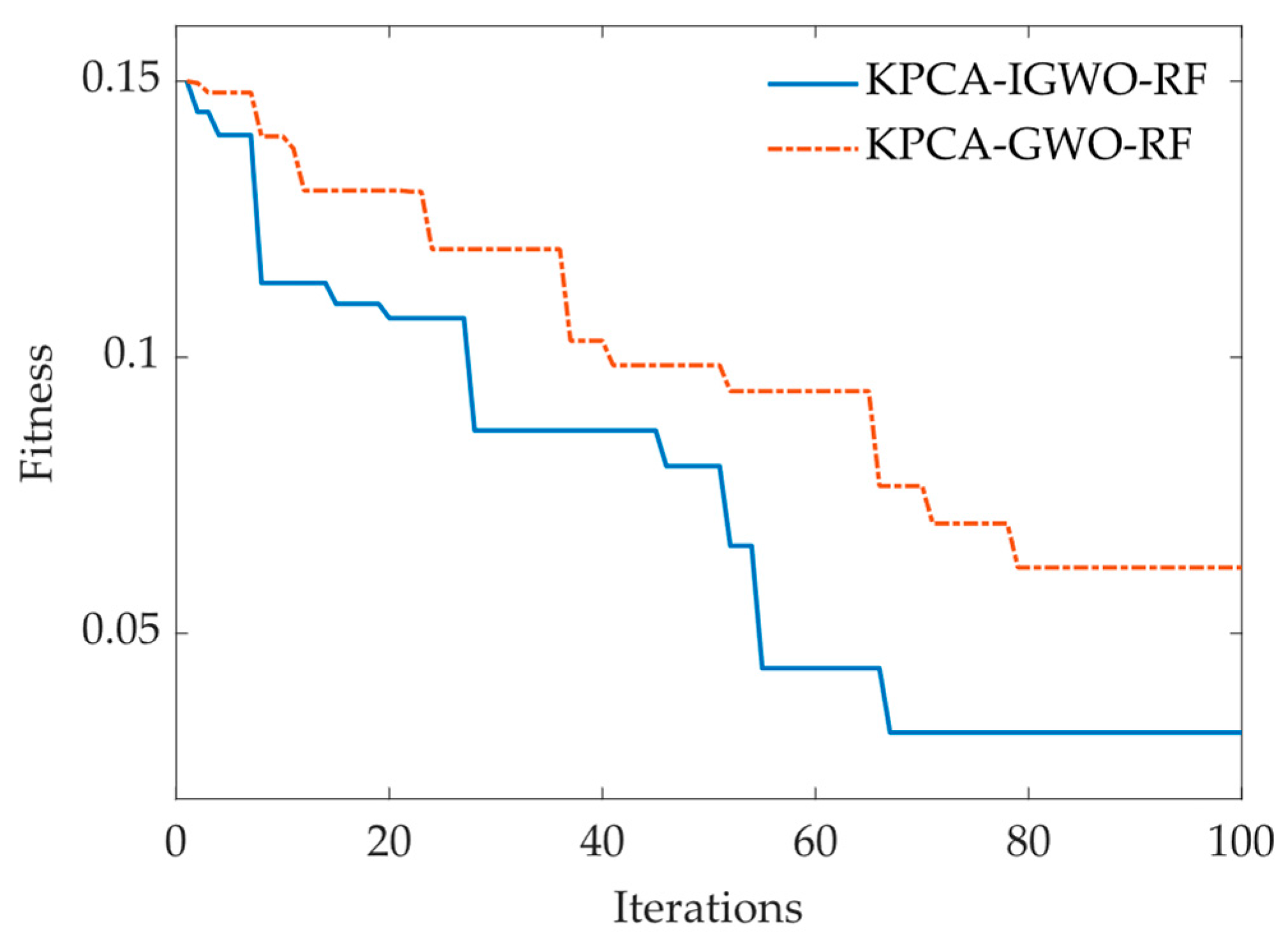
Based on the data in Table 2, it can be observed that the KPCA-RF model outperforms the traditional RF model, with an overall accuracy increase of 9% and a Kappa coefficient increase of 0.1167. The aforementioned observations arise from the utilization of 17 initial features as inputs in the RF model. These initial features exhibit a significant degree of interdependence, resulting in an abundance of redundant and overlapping information. To mitigate these issues, the proposed KPCA-RF model reduces the dimensionality of the initial features, effectively eliminating highly correlated data. By doing so, the interference caused by redundant information is mitigated, ultimately leading to notable enhancements in the overall identification accuracy. Nonetheless, the classification performance of the model is compromised due to the random assignment of initial parameters in the random forest algorithm. Moreover, incorporating the GWO algorithm to optimize the key parameters of dp and es in the RF model leads to an overall accuracy increase of 8.8095% and a Kappa coefficient increase of 0.0583. The KPCA-IGWO-RF model further enhances the performance by overcoming the issue of the GWO algorithm’s tendency to fall into local optimality. The model achieves the highest accuracy among all models, with an overall accuracy of 96.8% and a Kappa coefficient of 0.9667, which is 20.8% higher than the traditional RF model, and the Kappa coefficient increases by 0.2167. The iteration curves of the KPCA-GWO-RF and KPCA-IGWO-RF models are shown in Figure 8.
Figure 8 illustrates that the KPCA-IGWO-RF model becomes stable after 67 iterations, and the overall identification error rate of the model decreases to 0.032. The KPCA-IGWO-RF model achieves the minimum error rate earlier compared to the KPCA-GWO-RF model and escapes from the local optimal solution multiple times, resulting in a smaller final error rate. These results demonstrate that the IGWO algorithm can efficiently assist the model in achieving the optimal state more quickly and improving the model’s identification accuracy.

3.5. In Comparison to Other Existing Approaches

In order to further verify the effectiveness of the model proposed in this chapter in load identification, the model in this paper was compared with the LSTM-BP neural network proposed in the literature [13], and the SVM proposed in the literature [17], and the k-nearest neighbor (k-NN) proposed in the literature [26]. In order to facilitate a fair and rigorous comparison, the same dataset is employed to evaluate and compare the performance of the four algorithms under consideration. By utilizing a consistent set of data, any variations in the results can be directly attributed to the differences in algorithm design and implementation. This approach ensures a reliable and unbiased assessment of the algorithms’ respective capabilities and aids in drawing meaningful conclusions regarding their comparative effectiveness in load identification. The identification accuracy and Kappa coefficient of the four models are summarized in Table 3.
As illustrated in Table 3, the comprehensive identification accuracy and Kappa coefficient of the model employed in this chapter surpass those of the other three models. Furthermore, as the load quantity increases, the range of variation in identification accuracy exhibited by the model in this chapter is comparatively narrower compared to the other three models. The comparative analysis with existing literature further confirms the supremacy and resilience of the model presented in this chapter when addressing load-related scenarios.

4. Conclusions

In this study, we propose a non-intrusive load identification method based on KPCA-IGWO-RF, which utilizes the steady-state characteristic. To eliminate the information redundancy of the original data consisting of 17 characteristics, KPCA is employed to reduce the dimensionality of the data. RF is then utilized for load identification, and the IGWO algorithm is used to optimize the dp and es parameters of RF. The experimental results show that IGWO has a better global search ability than GWO. The KPCA-IGWO-RF model is evaluated based on the load identification accuracy and Kappa coefficient and is compared with other models. Future work will investigate the use of gradient boosting models as another possible ensemble approach due to their superior performance over random forest, as shown in many past applications [27,28].
Currently, our research focuses on evaluating the effectiveness of load identification using the collected dataset for training and testing purposes. However, in our future investigations, we aimed to explore the feasibility of implementing the algorithm on embedded devices. By doing so, we can enhance the practical applicability of the algorithm. Furthermore, we plan to leverage the complete energy management system facilitated by a cloud server architecture to further augment the practical value of the algorithm. This integration will enable a comprehensive energy management approach, enhancing the overall efficiency and effectiveness of the load identification and energy optimization.

Author Contributions

S.H. and G.Y.: Conceptualization, methodology, software, validation, formal analysis, investigation, data curation, writing—original draft preparation/review and editing; K.H., C.L. and M.W.: Conceptualization, methodology, visualization, supervision, project administration, funding acquisition. All authors have read and agreed to the published version of the manuscript.

Funding

This work was supported by the Natural Science Foundation of Hubei Province No.2022CFA007, and the Science and Technology Project of Hubei Province No.2022BEC017.

Data Availability Statement

Not applicable.

Conflicts of Interest

The authors declare no conflict of interest.

References

  1. Zhuang, D.; Gan, V.J.; Tekler, Z.D.; Chong, A.; Tian, S.; Shi, X. Data-driven predictive control for smart HVAC system in IoT-integrated buildings with time-series forecasting and reinforcement learning. Appl. Energy 2023, 338, 120936. [Google Scholar] [CrossRef]
  2. Tekler, Z.D.; Low, R.; Yuen, C.; Blessing, L. Plug-Mate: An IoT-based occupancy-driven plug load management system in smart buildings. Build. Environ. 2022, 223, 109472. [Google Scholar] [CrossRef]
  3. Schrenk, M.; Wasserburger, W.W.; Mušič, B.; Dörrzapf, L. SUNSHINE: Smart UrbaN ServIces for Higher eNergy Efficiency. In Proceedings of the GI_Forum, Rome, Italy, 20–23 May 2013; pp. 18–24. [Google Scholar]
  4. Athanasiadis, C.; Doukas, D.; Papadopoulos, T.; Chrysopoulos, A. A scalable real-time non-intrusive load monitoring system for the estimation of household appliance power consumption. Energies 2021, 14, 767. [Google Scholar] [CrossRef]
  5. Tekler, Z.D.; Low, R.; Zhou, Y.; Yuen, C.; Blessing, L.; Spanos, C. Near-real-time plug load identification using low-frequency power data in office spaces: Experiments and applications. Appl. Energy 2020, 275, 115391. [Google Scholar] [CrossRef]
  6. Hart, G.W. Nonintrusive appliance load monitoring. Proc. IEEE 1992, 80, 1870–1891. [Google Scholar] [CrossRef]
  7. Kamat, S.P. Fuzzy logic based pattern recognition technique for non-intrusive load monitoring. In Proceedings of the 2004 IEEE Region 10 Conference TENCON 2004, Chiang Mai, Thailand, 24 November 2004; pp. 528–530. [Google Scholar]
  8. Bonfigli, R.; Principi, E.; Fagiani, M.; Severini, M.; Squartini, S.; Piazza, F. Non-intrusive load monitoring by using active and reactive power in additive Factorial Hidden Markov Models. Appl. Energy 2017, 208, 1590–1607. [Google Scholar] [CrossRef]
  9. Wu, Z.; Wang, C.; Peng, W.; Liu, W.; Zhang, H. Non-intrusive load monitoring using factorial hidden markov model based on adaptive density peak clustering. Energy Build. 2021, 244, 111025. [Google Scholar] [CrossRef]
  10. Kosuke, S.; Shinkichi, I.; Tatsuya, S.; Hisahide, N.; Koichi, I. Nonintrusive appliance load monitoring based on integer programming. In Proceedings of the 2008 SICE Annual Conference, Tokyo, Japan, 20–22 August 2008; pp. 2742–2747. [Google Scholar]
  11. Hassan, T.; Javed, F.; Arshad, N. An empirical investigation of VI trajectory based load signatures for non-intrusive load monitoring. IEEE Trans. Smart Grid 2013, 5, 870–878. [Google Scholar] [CrossRef] [Green Version]
  12. Gillis, J.M.; Morsi, W.G. Non-intrusive load monitoring using semi-supervised machine learning and wavelet design. IEEE Trans. Smart Grid 2016, 8, 2648–2655. [Google Scholar] [CrossRef]
  13. Huang, L.; Chen, S.; Ling, Z.; Cui, Y.; Wang, Q. Non-invasive load identification based on LSTM-BP neural network. Energy Rep. 2021, 7, 485–492. [Google Scholar] [CrossRef]
  14. Fang, Y.; Jiang, S.; Fang, S.; Gong, Z.; Xia, M.; Zhang, X. Non-Intrusive Load Disaggregation Based on a Feature Reused Long Short-Term Memory Multiple Output Network. Buildings 2022, 12, 1048. [Google Scholar] [CrossRef]
  15. Popescu, F.; Enache, F.; Vizitiu, I.; Ciotîrnae, P. Recurrence Plot Analysis for characterization of appliance load signature. In Proceedings of the 2014 10th International Conference on Communications (COMM), Bucharest, Romania, 29–31 May 2014; pp. 1–4. [Google Scholar]
  16. Zhou, Y.; Sun, M.; Li, P.; Cui, W.; Liu, R.; Zheng, Z.; Jing, Z.; Zhu, H. Research on non-invasive load monitoring based on convolutional neural network. In Proceedings of the 2022 4th International Conference on Communications, Information System and Computer Engineering (CISCE), Shenzhen, China, 27–29 May 2022; pp. 472–477. [Google Scholar]
  17. Dufour, L.; Genoud, D.; Jara, A.; Treboux, J.; Ladevie, B.; Bezian, J. A non-intrusive model to predict the exible energy in a residential building. In Proceedings of the 2015 IEEE Wireless Communications and Networking Conference Workshops (WCNCW), New Orleans, LA, USA, 9–12 March 2015; pp. 69–74. [Google Scholar]
  18. Blanchard, G.; Bousquet, O.; Zwald, L. Statistical properties of kernel principal component analysis. Mach. Learn. 2007, 66, 259–294. [Google Scholar] [CrossRef] [Green Version]
  19. Guyon, I.; Weston, J.; Barnhill, S.; Vapnik, V. Gene selection for cancer classification using support vector machines. Mach. Learn. 2002, 46, 389–422. [Google Scholar] [CrossRef]
  20. Tekler, Z.D.; Chong, A. Occupancy prediction using deep learning approaches across multiple space types: A minimum sensing strategy. Build. Environ. 2022, 226, 109689. [Google Scholar] [CrossRef]
  21. Mirjalili, S.; Mirjalili, S.M.; Lewis, A. Grey wolf optimizer. Adv. Eng. Softw. 2014, 69, 46–61. [Google Scholar] [CrossRef] [Green Version]
  22. Li, Y.; Han, M.; Guo, Q. Modified whale optimization algorithm based on tent chaotic mapping and its application in structural optimization. KSCE J. Civ. Eng. 2020, 24, 3703–3713. [Google Scholar] [CrossRef]
  23. Rigatti, S.J. Random forest. J. Insur. Med. 2017, 47, 31–39. [Google Scholar] [CrossRef] [Green Version]
  24. Paul, A.; Mukherjee, D.P.; Das, P.; Gangopadhyay, A.; Chintha, A.R.; Kundu, S. Improved random forest for classification. IEEE Trans. Image Process. 2018, 27, 4012–4024. [Google Scholar] [CrossRef]
  25. Wan, T.; Jun, H.U.; Zhang, H.; Pan, W.U.; Hua, H.E. Kappa coefficient: A popular measure of rater agreement. Shanghai Arch. Psychiatry 2015, 27, 62–67. [Google Scholar]
  26. Tao, P.; Liu, X.; Zhang, Y.; Li, C.; Ding, J. Multi-level non-intrusive load identification based on k-NN. In Proceedings of the 2019 IEEE 3rd Conference on Energy Internet and Energy System Integration (EI2), Changsha, China, 8–10 November 2019; pp. 1905–1910. [Google Scholar]
  27. Low, R.; Tekler, Z.D.; Cheah, L. An end-to-end point of interest (POI) conflation framework. ISPRS Int. J. Geo-Inf. 2021, 10, 779. [Google Scholar] [CrossRef]
  28. Bentéjac, C.; Csörgő, A.; Martínez-Muñoz, G. A comparative analysis of gradient boosting algorithms. Artif. Intell. Rev. 2021, 54, 1937–1967. [Google Scholar] [CrossRef]
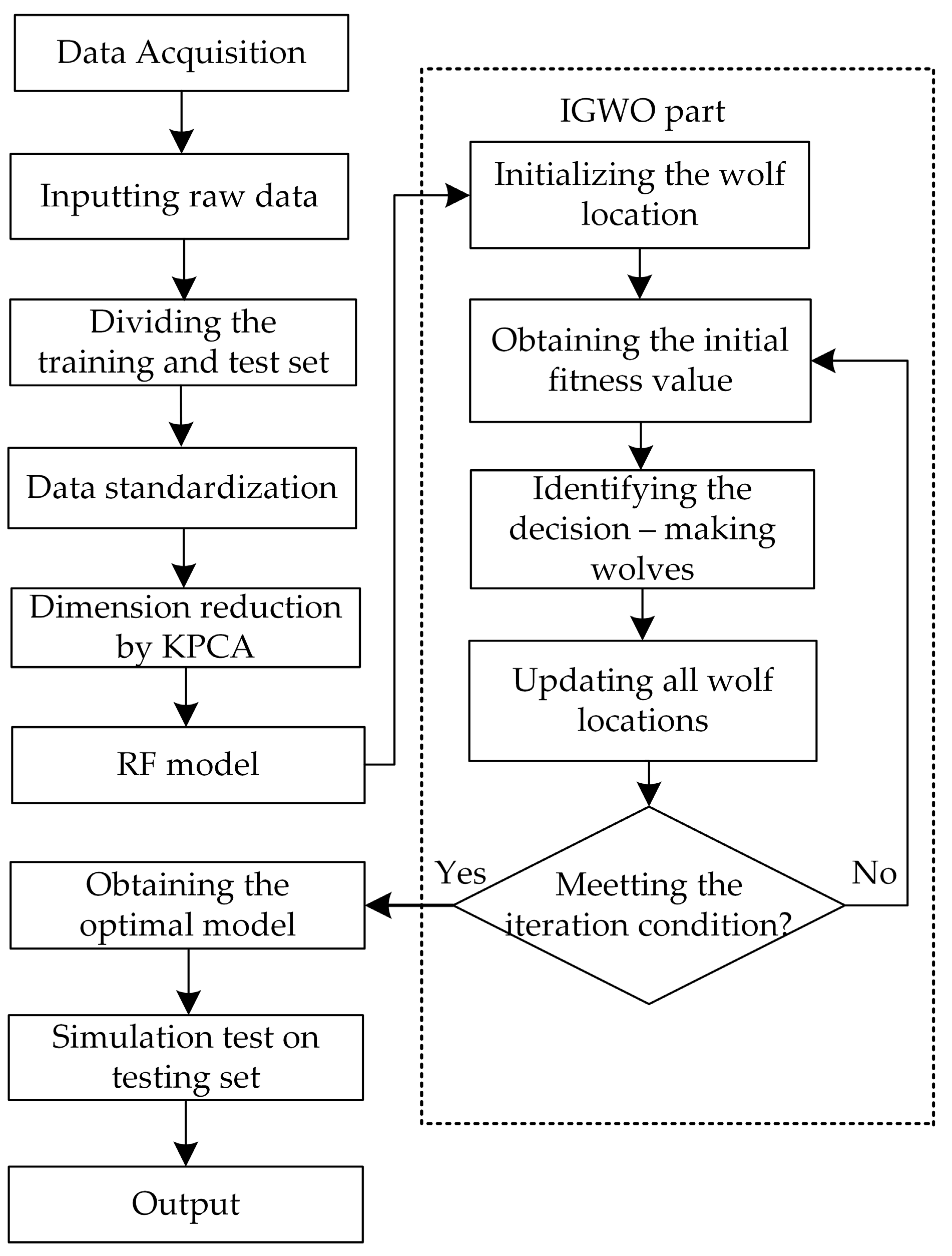
Figure 1. Flow chart of KPCA-IGWO-RF load identification model.
Energies 16 04805 g001
Figure 2. The arrangement of the power meter and electrical appliances.
Energies 16 04805 g002
Figure 3. Harmonic amplitudes of current when some devices are operating alone.
Energies 16 04805 g003
Figure 4. Harmonic amplitudes of current when some electrical appliances are run in combination.
Energies 16 04805 g004
Figure 5. Harmonic amplitudes of current at three gears of hair dryer.
Energies 16 04805 g005
Figure 6. The individual and cumulative contribution rate of each principal component.
Energies 16 04805 g006
Figure 7. The classification confusion matrix of KPCA-IGWO-RF model.
Energies 16 04805 g007
Figure 8. The iteration curves of the KPCA-GWO-RF and KPCA-IGWO-RF models.
Energies 16 04805 g008
Table 1. The combination of the load label and electric appliances.
One LoadTwo LoadsThree Loads
ConditionLabelConditionLabelConditionLabel
L11L1 + L211L1 + L2 + L319
L22L2 + L512L1 + L2 + L520
L33L5 + L213L1 + L2 + L921
L44L3 + L814L2 + L3 + L422
L55L5 + L715L3 + L4 + L823
L66L6 + L916L4 + L2 + L924
L77L8 + L1017L2 + L5 + L725
L88L8 + L918
L99
L1010
Table 2. Comparison of identification results of four models.
ModelAccuracy/%
One LoadTwo LoadsThree LoadsOverallKappa
RF73.666776.666778.5714760.75
KPCA-RF8595.833380.4762850.8667
KPCA-GWO-RF90.33339594.285793.80950.925
KPCA-IGWO-RF9697.083397.619096.80.9667
Table 3. Comparison of the identification results of four models.
ModelAccuracy/%
One LoadTwo LoadsThree LoadsOverallKappa
LSTM-BP9496.666790.9524940.9375
SVM93.666796.666781.428691.20.9083
k-NN90.333393.7588.571492.13330.9181
KPCA-IGWO-RF9697.083397.619096.80.9667
Disclaimer/Publisher’s Note: The statements, opinions and data contained in all publications are solely those of the individual author(s) and contributor(s) and not of MDPI and/or the editor(s). MDPI and/or the editor(s) disclaim responsibility for any injury to people or property resulting from any ideas, methods, instructions or products referred to in the content.