Article

Electric Water Heater Modeling for Large-Scale Distribution Power Systems Studies with Energy Storage CTA-2045 Based VPP and CVR

1
SPARK Laboratory, ECE Department, University of Kentucky, Lexington, KY 40506, USA
2
ABB USRC, Raleigh, NC 27606, USA
3
A. O. Smith Corporation, Milwaukee, WI 53224, USA
*
Author to whom correspondence should be addressed.
Energies 2023, 16(12), 4747; https://doi.org/10.3390/en16124747
Submission received: 12 May 2023 / Revised: 6 June 2023 / Accepted: 8 June 2023 / Published: 15 June 2023
(This article belongs to the Section D: Energy Storage and Application)

Abstract

:
As the smart grid involves more new technologies such as electric vehicles (EVs) and distributed energy resources (DERs), more attention is needed in research to general energy storage (GES) based energy management systems (EMS) that account for all possible load shifting and control strategies, specifically with major appliances that are projected to continue electrification such as the electric water heater (EWH). In this work, a methodology for a modified single-node model of a resistive EWH is proposed with improved internal tank temperature for user comfort modeling and capabilities for conservation voltage reduction (CVR) simulations as well as Energy Star and Consumer Technology Association communications protocol (CTA-2045) compliant controls, including energy storage calculations for “energy take”. Daily and weekly simulations are performed on a representative IEEE test feeder distribution system with experimental load and hot water draw (HWD) profiles to consider user comfort. Sequential controls are developed to reduce power spikes from controls and lead to peak shavings. It is found that EWHs are suitable for virtual power plant (VPP) operation with sustainable tank temperatures, i.e., average water temperature is maintained at set-point or above at the end of the control period while shifting up to 78% of EWH energy out of shed windows per day and 75% over a week, which amounts to up to 23% of the total load shifted on the example power system. While CVR simulations reduced the peak power of individual EWHs, the aggregation effect at the distribution level negates this reduction in power for the community. The EWH is shown as an energy constant load without consistent benefit from CVR across the example community with low energy reductions of less than 0.1% and, in some cases, increased daily energy by 0.18%.

1. Introduction

Electricity is the art of equilibrium as the supply and demand have to match each other at any given moment. Failing to do so will lead to voltage violation, power outage, or even the damage of user appliances and facilities of the power system. The power demand in a utility’s service area depends on seasonal and timely factors. It is highly predictable at feeder level as the aggregated user behavior offsets the randomness from individual users.
In recent years, renewables have been penetrating the power system in a steady trend [1]. The intermittent nature of renewable generation requires the grid operators to respond quickly to provide the right amount of power through curtailment or increased generation. Curtailing surplus generation is straightforward, unlike when the renewable generation suddenly drops, the grid operators are left with no choice but to run the expensive backup generators. Doing so might still not be enough when the gap left by renewable generation is too large.
One potential solution is from the demand side by grouping residences as a virtual power plant (VPP). A VPP offers deeper integration of renewables and demand flexibility than traditional approaches. Residences in a VPP can share any local power generation and offset the peak demand within the subsystem through smart controls. These neighborhood-based VPPs also have several challenges, for example, the residences are located in the same area, and therefore, all the local renewable generators experience the same external weather conditions. As a result, all the local renewable generators in a VPP will have the generation peak at the same time. When the penetration of renewable generation is high, the VPP will be unable to retain the surplus local generation. Secondly, it is more likely the residences in the same neighborhood have similar power usage pattern. When houses with similar user pattern are aggregated, the peak power is more likely to be amplified.
Energy storage systems (ESSs) are a potential solution to mitigate these aggregation effects on residential VPPs. Another application of energy storage is the assessment of melting of phase change in latent heat storage technology [2]. Residential ESSs have been shown to store the surplus VPP power generation and supply the peak demand [3]. Battery systems are expensive for both initial investment and maintenance, thus, will not be discussed in this paper.
Instead, focus is placed on the adoption of ubiquitous electrical water heaters (EWHs) as energy storage. The water tank provides large thermal mass and, when controlled as energy storage, there is more flexibility for the homeowners to better adjust to market prices, such as time of use (T.O.U.), and for utilities to implement VPP. Alternative heating element designs in EWHs have been considered to improve the thermal energy storage and dispersion of heated water in the tank [4]. Detailed thermo-hydraulic studies have also been conducted to quantify the natural convection patterns of water in the EWH tank [5] and support regions of water remaining cooler underneath the heating element, as accounted for in this paper through the proposed modified single node model.
Through smart controls, such as Consumer Technology Association protocol 2045 (CTA-2045) for demand response (DR) [6], water heaters can avoid being turned ON during the peak hours by preheating or postponing the heating process. When local renewable generation is available, water can be preheated and the water heater can perform as thermal ESS. When the heating process is postponed, the standby loss reduces because the water in the tank has less thermal energy to lose, and—in the case of heat pump water heaters—recovery efficiency increases by sending colder water to the compressor unit [7]. A second method for energy storage controls considered in this paper is conservation voltage reduction (CVR) for EWH, where the supply voltage to the appliance is reduced in an effort to mitigate load and provide grid services, such as load shifting and energy savings.
A research gap remains as some previous studies did not consider that some homes might not be able to participate in the DR due to the tank temperature and hot water draw (HWD) of that home, i.e., that if tank temperatures dropped below a comfort limit to ensure hot water, the home would remove itself from the controls. Additionally, the grid impacts are different even for the same homes when they are connected to different nodes in the distribution system. Previous studies usually left the temperature inside the water tank different from its original status after control [8]. Such control is not sustainable as the water temperature might be too low in the beginning of the next day. User behavior typically has a week-long cyclical pattern. Previous studies for EWH control usually focused on the daily performance and did not consider long-term controls.
The problems addressed by this paper are within the smart grid transition specifically, the development of VPP controls to improve grid resilience and reliability. A main difficulty with VPP controls is the security for data transfer and interoperability of residential ESS devices. This paper aims to solve this problem with the development of industry communication protocol compatible VPP controls for one of the major residential appliances and ESSs, the EWH. To do so, another problem must be solved, the development of an ultra-fast and satisfactorily accurate EWH model methodology that is scalable to large numbers of homes on a residential electric power distribution system, which also has realistic load, hot water draw (HWD) profiles, and user comfort limits.
This paper includes the following contributions, such as a modified ultra-fast single-node EWH model suitable for large-scale power system studies with improved thermal flexibility estimation while considering user comfort; a methodology for evaluating CVR for resistive EWHs; daily CVR simulations on the IEEE 123 bus benchmark distribution system [9] with experimental residential load and HWD profiles; development of a VPP control framework compatible with short-term and long-term simulations, which considers water temperature for user comfort; two case studies for daily and weekly CTA-2045 based VPP on the benchmark distribution system; and the development of sequential controls for peak mitigation using CTA-2045 standards. The structure of this paper is as follows. A technology review of smart controls and previous studies in Section 2, methodology formulation in Section 3, description of benchmark system used in all simulations in Section 4, and CVR and CTA-2045 smart control daily and weekly simulation results in Section 5, Section 6 and Section 7. Furthermore, included is a discussion for sequential control development in Section 8 followed by our conclusions.

2. Technology Review

The EWH is an important component in the achievement of effective home energy management [10,11]. The storage capacity of water heaters is determined by the volume of the water tank, and the the total electricity used by EWHs is determined by the user behavior, i.e., the thermal energy reduction from hot water leaving the tank should be almost equal to the electricity used for heating, given a near 100% insulation. The large thermal mass of storage tanks in water heaters enables flexibility in the timing of heating processes. An accurate and ultra-fast model is needed to understand the impact on the hot water storage temperature when the controls are modified. The modeling of these water heaters needs to consider climates zones, conditioned and unconditioned spaces, hot water usage profiles, and water heater types, such as gas storage, gas tankless, condensing storage, electric storage, heat pump, and solar water heaters [12].
The model should also be flexible to represent water heaters with different properties, i.e., tank volume and rated power. When adopted in a transactive and large-scale systems, the trade-off between accuracy and computational complexity of a EWH model must be considered. Specifically, Mukherjee et al. considered a partial differential equations (PDE) model, which could be, in principle, more accurate [13]. They also reach the conclusion that the model is infeasible for large-scale evaluation studies, such as the IEEE 123 bus system due to excessively long computational times. They recommended that much faster one-node models could be employed as an alternative because they exhibit similar consumption. For this reason, a modified single-node EWH model is proposed in this paper for large-scale simulations of EWH smart controls.
Previous studies into smart controls for EWHs show that two concerns should be kept in mind when implementing water heater controls for a community. The first concern is also the bottom line for field deployment—the domestic hot water temperature should never be too low [14]. Secondly, the limited access to real-time data—due to either hardware limit or privacy concerns—is a significant obstacle [15]. Additionally, a control method for large water tanks might not work properly for small water tanks—the temperature for water inside the small tank might drop or increase too fast before the goals of control are achieved [16].
Successful studies into EWH smart controls include a centrally adapted control model which avoided the peak power by scheduling each EWH, thereby reducing the peak load of 1.05 kW/EWH to 0.4 kW/EWH [17] and a deep Q-networks algorithm for water heaters under T.O.U pricing that showed electricity cost savings up to 35% [18]. Other recent examples of EWH controls to reduce grid impact from electric vehicles (EV) show that thermal energy storage is viable to improve grid operation, given the smart technology to control them is in place [19,20].
Furthermore, planning the temperature inside the water tank could reduce the energy usage by up to 11% without compromising the user comfort [21]. In practice, the temperature in the water tank is stratified and therefore, hard to measure. This is mitigated by viewing the EWH as general energy storage (GES) capable of following Energy Star and ESS calculations, such as equivalent state-of-charge (SOC) and “energy take” as proposed in this work. An advantage of this modeling approach is that the EWH may be integrated into unified ESS controls through the CTA-2045 protocol. Previous reports, including field deployment in [15,22], show that industry has interest in developing further the CTA-2045 communication protocol and there is support for widespread adoption. A preliminary case study by this same group of authors using CTA-2045 for GES-based controls of a large group of EWHs in a modified IEEE-123 bus system [23] is detailed in this paper to address the bouncing effect of spikes in power following control periods with sequential implementation.
As for the second type of EWH controls considered in this paper, traditional implementation of CVR was to reduce the voltage across an entire distribution feeder, thus, lowering the power to the entire residential load [24,25,26]. In these works, CVR is evaluated using comparison-based, regression-based, synthesis-based, and simulation-based methods. Stochastic evaluations are employed to analyze the impact on feeders and select ones for the highest benefit. Another study suggests that heavily loaded and higher voltage feeders should be targeted for the deployment of CVR as it had the most benefits [27] and recent capacitor placement and optimization techniques are underdevelopment to support these CVR efforts [28]. A detailed review is provided for CVR modeling approaches; the potential for use with low-income communities; and the steps to complete CVR studies, building or updating circuit modeling, calibrating water heater models, simulating with and without controls, and comparing for savings [29].
With the increasing penetration of DERs, one approach has been to adapt CVR studies to include Volt/Var controls and assess the influence of sudden changes in power [30,31]. Another approach has been to apply CVR to select appliances or loads for maximum impact. In these studies, it is important to consider the category of load because constant current and resistance loads show the best results and constant power or energy loads have with very little response to CVR in terms of energy reduction [32]. While EWH’s are constant energy loads, there has been interest in CVR for them as they make up a significant portion of residential load. An example of research into CVR at the appliance level demonstrated reduced power from switching between 220 V to 110 V supply for EWHs in partnership with PNNL [33] across an entire day.
Another previous case study of 1000 EWH shows a 14% reduction in ZIP load, when the voltage was changed from 124 V to 116 V [34]. One issue with this study and other ZIP-model-based simulations for CVR is that it is common for the ZIP modeling to stop heating before tank temperature is reached as the same stop time is maintained with reduced power, which does not ensure the same amount of energy is transformed from electricity to thermal energy [35]. Within this paper, in addition to smart control development based on communication standards, benchmark CVR simulations are completed with a physics-based EWH model validated against experimental results to show that EWH load is energy constant and will not have significant reduction in energy and why.

3. Ultra-Fast Model for EWH and Energy Storage Employing CBECC-Res Typical Water Draw Profiles

While detailed studies into complex EWH thermal modeling focuses on the number of thermal nodes accounted for [36] and thermal accuracy comparisons have been made [37] for single EWHs, benchmark satisfactory models for large-scale simulations are still needed. Mukherjee et al. found that advanced physics-based EWH models, such as partial differential equations (PDE), are complex and require significant computational power, which makes them unfit for smart grid community modeling with hundreds of homes in co-simulation or with real-time purposes [13]. They assert that thermally stratified, two-node, and single-node models serve as ultra-fast alternatives for estimations of power and grid impact with small variance in the consumption results from the more advanced methods at the community level. Therefore, a modified single-node model has been selected with the lowest number of parameters for large-scale simulations to estimate the impact of smart controls on the electric distribution system, while considering natural water convection patterns.
The single-node model, in the form of a gray-box RC thermal model, has been validated against experimental resistive EWH results from smart control testing Of CTA-2045 based controls conducted by EPRI and NREL [38]. A modification for improved thermal flexibility estimation is proposed in this work. Satisfactory simulation of smart controls based on CTA-2045 communication standard and energy take limits for heating element operation employing the proposed model are visualized in Figure 1, specifically “normal operation” without controls and “load-up” cases. During load-up periods additional energy is accepted from the grid and stored—as opposed to “shed” cases where reduced energy is drawn from the grid and stored energy used to meet the HWD.
The water tank volume, V (m3); density of water constant, ρ (993 kg m 3 ); specific heat capacity of water, c p (4179 J kg   ° C ); the average temperature in the water tank at time t with time steps of one minute, θ T ( ° C ); and a thermal region coefficient, η (0.9), are used to calculate the thermal energy stored in the EWH, E W ( t ) , following:
E W ( t ) = V · ρ · η · c p · θ T ( t ) .
The thermal region coefficient has been proposed to account for typical heating thermodynamics of the water tank. The tank volume underneath the heating element does not warm up or store a significant amount of energy and may be neglected in the energy calculations to improve the modeling of the thermal flexibility and internal tank temperature with a single node model. The individual internal tank temperature and EWH power are calculated considering affects from input electric power, standby heat loss, outlet flow mixing with cold water, and hot water draw (HWD) activities.

4. Benchmark Distributions System with Representative HWD and Load

To unify the CTA-2045 smart controls of the EWH with GES so that a single energy management system for thermal and electric energy storage may be employed, Energy Star calculations are required for the energy a storage system may accept before reaching capacity at a given time, i.e., “energy take”. For the EWH, the maximum capacity is determined based on the temperature in reference to the maximum temperature of hot water allowed per user settings. It is proposed to use the initial tank temperature as the reference point for large studies to avoid challenges associated with user input data collection and allow for the adaption of the maximum tank temperature as part of the control development. The energy take, E T , W ( t ) , is calculated as
E T , W ( t ) = E W , i ( 0 ) E W ( t ) ,
where the E W , i ( 0 ) is the thermal energy stored per EWH at the start of the simulation. The energy take per EWH calculated in this manner may be compared to control limits, Q T , m i n ( t , H W D ) , Q T , m a x ( t , H W D ) to determine the status of the heating element as follows:
S ( t ) = 1 , if S ( t 1 ) = 0 & E T , W ( t ) Q T , m a x ( t , H W D ) 0 , if S ( t 1 ) = 1 & E T , W ( t ) Q T , m i n ( t , H W D ) S ( t 1 ) , otherwise ,
where S ( t ) is the status of the EWH, either ON at binary one or OFF at binary 0, and H W D is the hot water draw at that time, t. Using these controls, the CTA-2045 controls may be applied by associating Q T , m i n ( t , H W D ) , Q T , m a x ( t , H W D ) limits to DR operations.
The single-node model has also been expanded to include behind-the-meter (BTM) voltage adjustments to the EWH as part of community-wide CVR testing. The power draw of the EWHs is reduced through reduction in voltage supplied to the device. The adjusted EWH power, P E W H ( t ) , is calculated following these voltage changes as
P E W H ( t ) = P r V r I r · C V R j ( t ) · V r V H ( t ) ,
where P r , V r , and I r are the rated power, voltage, and current; C V R j ( t ) is a coefficient to adjust the voltage based on percent reduction, j; and V E W H ( t ) is the voltage experience by the EWH. C V R j ( t ) is defined by:
C V R i ( t ) = ( 1 j 100 ) .
The gray-box RC model incorporates the P E W H ( t ) to calculate the change in tank temperature as follows:
C d θ T ( t ) d t = S ( t ) · P r ( t ) · C V R i 1 R [ θ T ( t ) θ A ] ρ c p W ( t ) θ T ( t ) θ W , C ,
where θ T ( t ) is the tank temperature, θ A is the temperature of the ambient air; θ W , C is the temperature of cold inlet water; and R , C are the equivalent thermal resistance and capacitance of the EWH tank. In this formulation, both the impact of the CTA-2045 and CVR controls on the tank temperature and energy storage are considered. This proposed single node model has been integrated into a co-simulation framework for VPP operation of hundreds of homes through CTA-2045 and CVR control case studies in this paper (Figure 2).
Within this paper, the proposed methodology has been applied to a benchmark distribution system (Figure 3a), the IEEE 123 bus [9], in OpenDSS using the Python plug-in to establish sustainable EWH controls based on industry standards for DR. In a previous paper by the authors [23], including preliminary CTA-2045 controls case studies, the original load across all nodes was replaced with a total of 353 residential load profiles, each with a maximum power usage of 10 kW or less from the SET project [39], a large experimental dataset of more than 5000 homes. Only profiles with typical residential daily usage of 20 to 40 kWh and no missing data points are selected. This work has been expanded to include the described modifications to the single-node model for improved characterization of the thermal energy flexibility and CVR controls. The simulation length has also been increased to include week-long studies, each day with a unique profile from the SET homes for both weekday and weekend types.
For the control simulations, each home is equipped with a 5.5 kW smart EWH with a rated power, a tank size of 50 gal., and the initial water temperatures in the tanks are evenly distributed between 46 and 57 °C. The equivalent thermal resistance of the water heaters was assumed to be 1400 °C/kW. These parameters were selected to emulate a physical A.O. Smith resistive EWH used in studies by NREL and EPRI for preliminary testing of CTA-2045 Standard commands, as described in Section 3.
Realistic HWD profiles are assigned to each home from the 2019 CBECC-Res large dataset [40]. Profiles from homes with different numbers of bedrooms (1–5) and occupancy, as well as day of the week, are used to build a representative community for testing. An example HWD profile with subsequent EWH power and temperature are visualized in Figure 3b. The Q T , m i n ( t , H W D ) , Q T , m a x ( t , H W D ) limits for controlling the heating element in each EWH per CTA-2045 case are described in Table 1. The energy take limits were calculated to ensure a heating or cooling time around five minutes for the realistic load-up and 15 min for the maximum load-up case using the the proposed single node model that was validated against a physical EWH. Further evaluation of these limits for alternate VPP peak power reduction performance over larger or shorter time periods is discussed in Section 8.

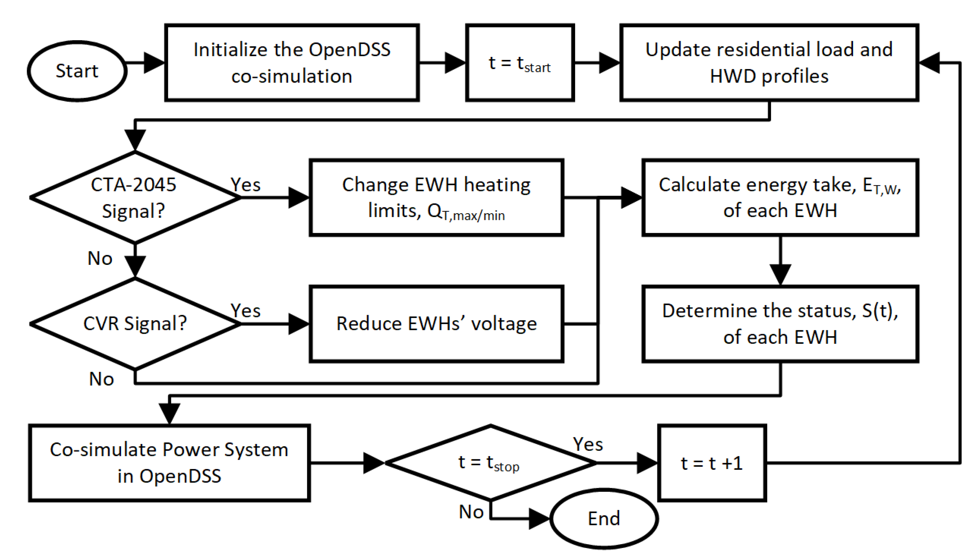
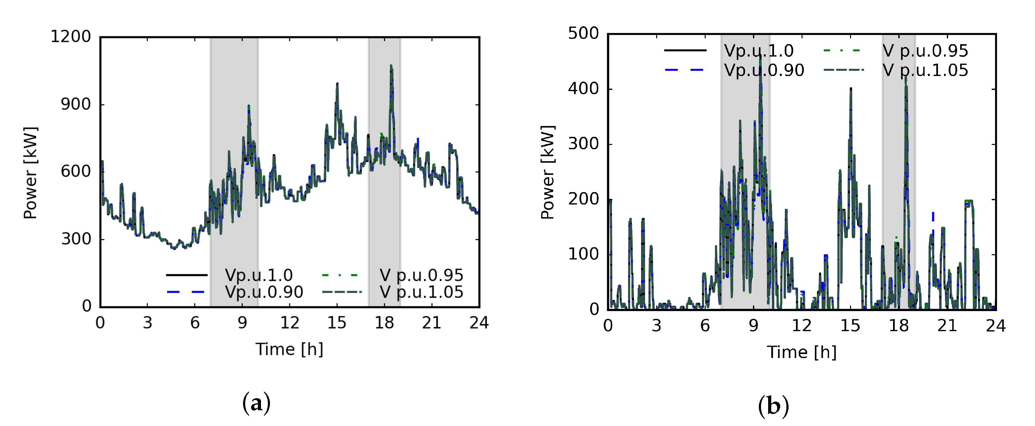
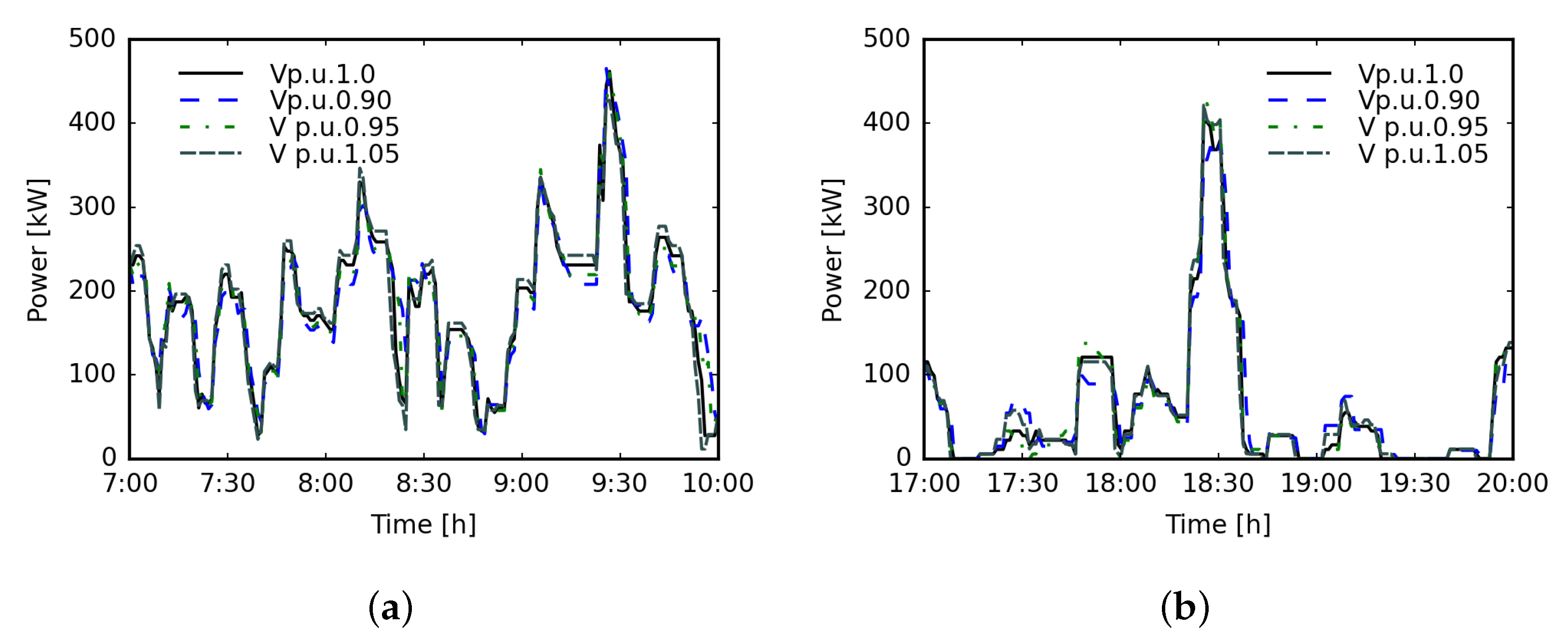
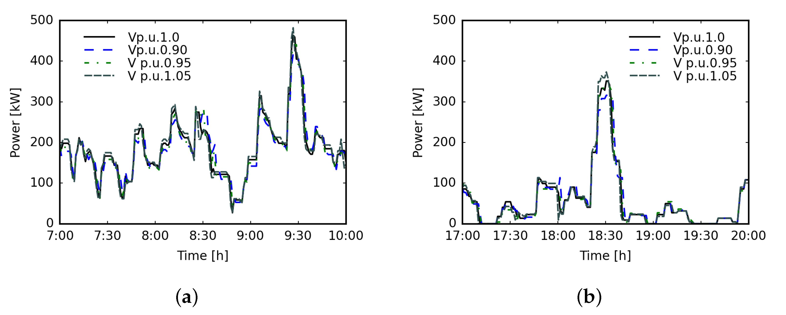
5. Conservation Voltage Reduction (CVR) EWH Simulations

CVR simulations have been conducted to assess power shifting and energy savings capabilities by reducing the per unit (p.u.) voltage to the EWH at each home in the residential benchmark system. Normal operation controls based on the energy take of each EWH for GES modeling is employed to determine the status of the EWH heating elements, and the EWH voltages are reduced through CVR during DR periods. Voltages were varied from 0.90 to 1.05 p.u. by increments of 0.05 p.u. All cases are compared to rated voltage of 1.0 p.u. or 120 V. The representative synthetic community was used with profiles from a Wednesday and were assumed able to receive a CVR command signal from the utility. CVR periods of 7 to 10 and 17 to 20 military time were selected to reduce common work week peak time load. This is especially important as these times may become frequent EV charging windows as people prepare to leave for work, and utilities would benefit from reduced loads from other appliances.
During the CVR simulations, the status of operation (ON/OFF), tank temperature, and energy take were considered for the individual homes. An example of individual home EWH power temperature and energy intake are illustrated in Figure 4 during the CVR morning time window.
The magnitude of the power changes and the rate at which the energy take and temperature adjusts is also affected by the voltage change, i.e., the EWH remains ON for longer as the power decreases to make up for the slower change in tank temperature. This demonstrates that the energy, visibly seen as the area under the power curve, remains constant to physically heat the water to the desired temperature and energy usage range for human comfort. In previous CVR case studies, this effect was not captured as a modeling insufficiency with ZIP parameters and power is shown to stop at the same time regardless of supplied voltage and decreased power [35]. This is indicative that the requirements of the tank to meet the set comfort temperature point were not adequately considered in previous studies. The controls proposed in this CVR simulation are based on the individual energy usage of the EWHs and address this research gap.
The aggregate total power as simulated at the main feeder and calculated community EWH power is illustrated in Figure 5 with the 0.95 p.u. case in green to represent the lowest allowed voltage per USA grid operation standards. The CVR periods are visualized by grey shading and since the change in power is so small, zoomed in plots of EWH power during the CVR time windows are provided in Figure 6. Peak load from the EWH is reduced from the 1.0 p.u. case during portions of the time window, while at other times the power is increased. The peak power demand for the EWH actually increased in the 0.95 Vp.u. case by 0.47%. This indicates that CVR for EWH may not be successful at reducing aggregate peak power for the EWHs across a community consistently. The peak power was not reduced due to longer heating times as more EWHs are heating during spikes in demand as compared to the baseline case (Figure 7). In summary, CVR may only be successful to shift peak across an hour or more time window, if the human behavior-based HWD profiles are spread out enough that the CVR does not cause additional overlap between EWH heating times in response to comfort limits.
Other factors that may influence the impact of the CVR are the rated power of the water heaters and their individual thermal resistivity. To test the effects of these factors, the CVR simulations were repeated with 4.5 kW rated power and increased thermal resistivity at 1500 °C/kW (Figure 8). In this scenario, the CVR successfully reduces the peak load in the morning at 9:30 for all cases from 1.05 down to 0.90 p.u.; though in line with the previous scenario, the power over the entire window is inconsistent for reductions. The number of additional houses requiring heating was still affected if the CVR was able to reduce the aggregate power, as seen in Figure 9.
In both cases, the energy across the community was shown to be minimally affected by the CVR, and this is further explained by the individual EWHs remaining in the ON operation for longer as the voltage p.u. decreases (Figure 10).
Additionally, the EWHs heat for approximately 11 min longer in the 4.5 kW case than the 5.5 kW case. The timing of the EWH’s switching ON and OFF affects how the peak is shifted and not all combinations lead to peak shifting success at the community level. Overall, adjusting the rate of power and thermal resistivity to represent smaller, more thermally efficient EWHs did not lead to more effective power sifting or energy savings. From our simulations, further CVR studies BTM would be more impactful on loads where the amount of energy required to satisfy the consumer’s comfort limits does not remain constant, such as cases with dimmer lights where the energy does not have to be recovered.
The impact on the total energy used by the EWH is not indicative that energy will be reduced as all fluctuations in energy use are less than 0.02%. Additionally, more energy is required when the voltage to each EWH is the lowest (Table 2). The CVR factors, a metric commonly used to evaluate the effects of the voltage controls, is very low. As a result, the authors can not conclude that the total energy required by the utility is significantly changed by CVR on EWHs in this benchmark study. Since EWH’s require a constant amount of thermal energy to heat and maintain the hot water in the tanks across the community, reducing instantaneous active power does not change the amount of demand for electrical energy.

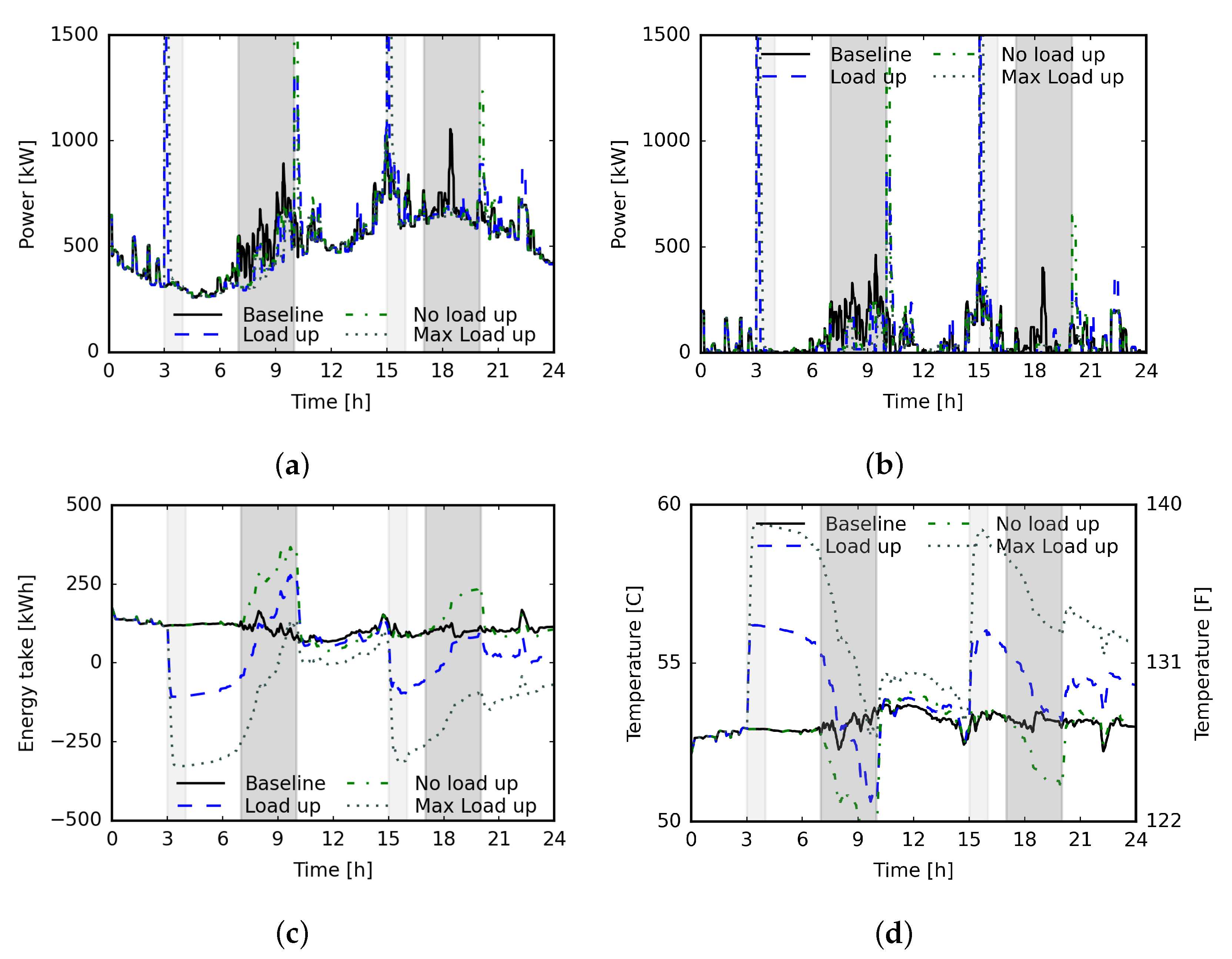
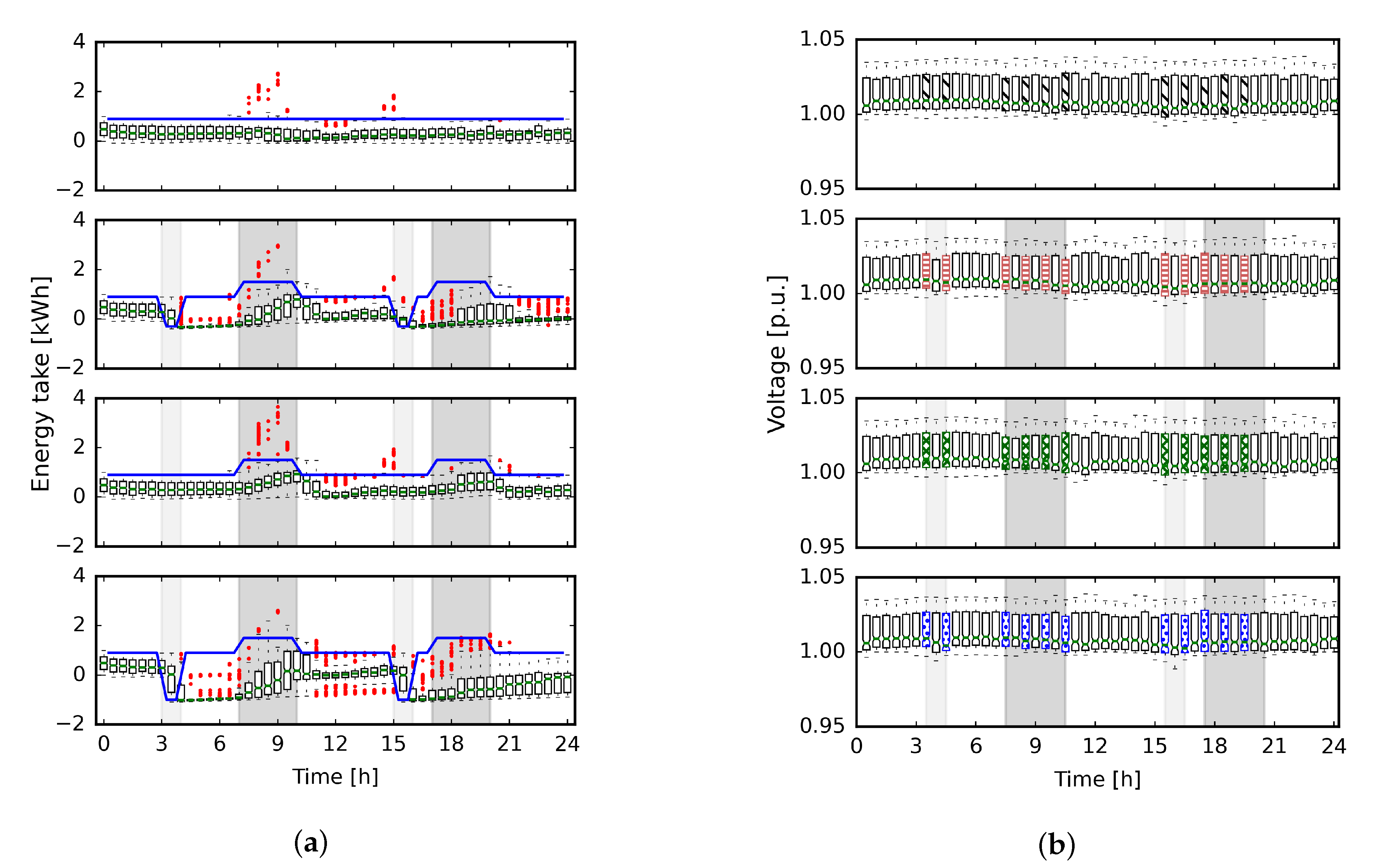
6. Daily VPP for a Full Day Schedule

Virtual Power Plant (VPP) applications of EWHs have potential for load shifting when considering CTA-2045 commands and the ability to preheat the water stored. Three case studies were conducted on the same time period of 24 h as the CVR simulations, i.e., a Wednesday during the summer as described in Section 4. Control windows for “load-up” were selected to pre-heat the water before the “shed” commands, specifically from 3 to 4 at night and 15–16 during the afternoon. Shed windows were selected from 7 to 10 a.m. and 17–20 to alleviate peak time stress from before work and return home activities.
The operation of the heating elements in the community are controlled by the energy usage limits described in Table 1. These values were selected based on the length of time it takes to heat the water from the initial value to the temperature corresponding to the energy take limit, i.e., approximately five minutes to heat to −300 Wh and 15 min to heat to −1000 Wh. The water temperatures are 128 and 133 °F, both of which are well below the maximum temperature of 165 °F that was considered in previous studies with a mixing valve in a residential setting [22]. The higher the maximum setpoint selected, the more thermal energy is stored in the tank and the longer the EWHs will need to operate. This leads to higher spikes during the day and less chance of mitigation through sequential controls.
During the load-up period, a CTA-2045 standard command is sent to each EWH in the community to decrease the energy take limit, Q T , m i n ( t , H W D ) , and increase the thermal energy stored. This will cause all the EWH to start at once to raise the equivalent SOC of the VPP across the community. In Figure 11, the aggregate power spikes to more than double the original base load in the distribution system at the start of the load-up period. The EWH load is subsequently decreased during the shed period as the water was pre-heated to decrease the energy take of the equivalent VPP thermal battery. At the end of the shed control period, the power spikes again as the EWHs turn ON to return the energy take and temperature to the normal operation range.
While the power is mitigated during the shed time period, the large spikes from the load-up and following the end of the shed are not suitable for deployment and may cause issues to the utility for meeting the sudden brief spike in demand. Sequential controls are proposed to accomplish the same shed in power incrementally. A systematic search was completed to select a batch size of 24 houses, each deployed every 4 min to phase in for all homes in an hour. Other combinations of batch size and phase-in time are feasible with drawbacks such as slower reaction time to shed commands and longer load-up periods. Further discussion is provided in Section 8.
Throughout the simulation, the state of each individual EWH’s energy usage and subsequent internal water temperature is considered (Figure 12). The order of the cases in the subplots is as follows, baseline, realistic load-up, no load-up, and maximum load-up. The sequential controls are visible in Figure 12a, and the temperatures across the community are seen increasing during the load-up and falling during the shed. The number of houses with average temperatures below 35 °C increase in all three cases as compared to the baseline. This is acceptable in the controls as the EWHs are set to kick on during shed if the energy take limits are violated to reduce the disruption to hot water availability as much as possible, and the users are assumed to be compensated for more relaxed service during shed times.
One of the contributions of this study is that the CTA-2045 commands are evaluated and simulated at each individual EWH in the community through object-oriented programming and class variables. The sequential operation of the EWHs across the community as well as their internal tank temperatures are visualized in Figure 13. The red dots are outliers in the distribution of temperatures that are beyond the quartile range at that time (t), and should not be read as comfort violations. In this approach, each tank evaluates its internal energy tank level and opts into the community DR events as possible per comfort standards for realistic community impact analysis and individual home status assessments. The energy take distributions and the limit, Q T , m i n ( t , H W D ) , for EWH heating operation to turn ON are visualized by the boxplot with blue lines in Figure 14. The outliers above the maximum limit are the EWHs that still require heating during the shed. Through this method, human comfort expectations to have hot water on demand are ensured. Additional analysis of temperature and energy usage selection in the controls is described in Section 8.
The voltage across the system is unaffected by the controls as seen close up in Figure 15 with no voltage violations. The developed sequential controls reduced the spike caused by the load-up to below the original base peak in the morning, making it more feasible from a grid impact perspective. The EWH power demand was successfully shifted from peak times to the load-up times selected at night and mid-afternoon. The temperature and energy usage levels were returned to normal operation ranges at the end of the period. The maximum load-up case serves as a test of the ability of the EWH to shift the load from additional pre-heating. In comparison to the no load-up case where 21 MWh, 48.3%, of demand is shed, the maximum case reduces the load during shed periods by 34 MWh, 78.9%, while the realistic load-up reduces it by 28.6 MWh, 65.5%. This indicates that the pre-heating of water is conducive to further load shifting grid services, and, thus, in future simulations, the no load-up case will not be considered.

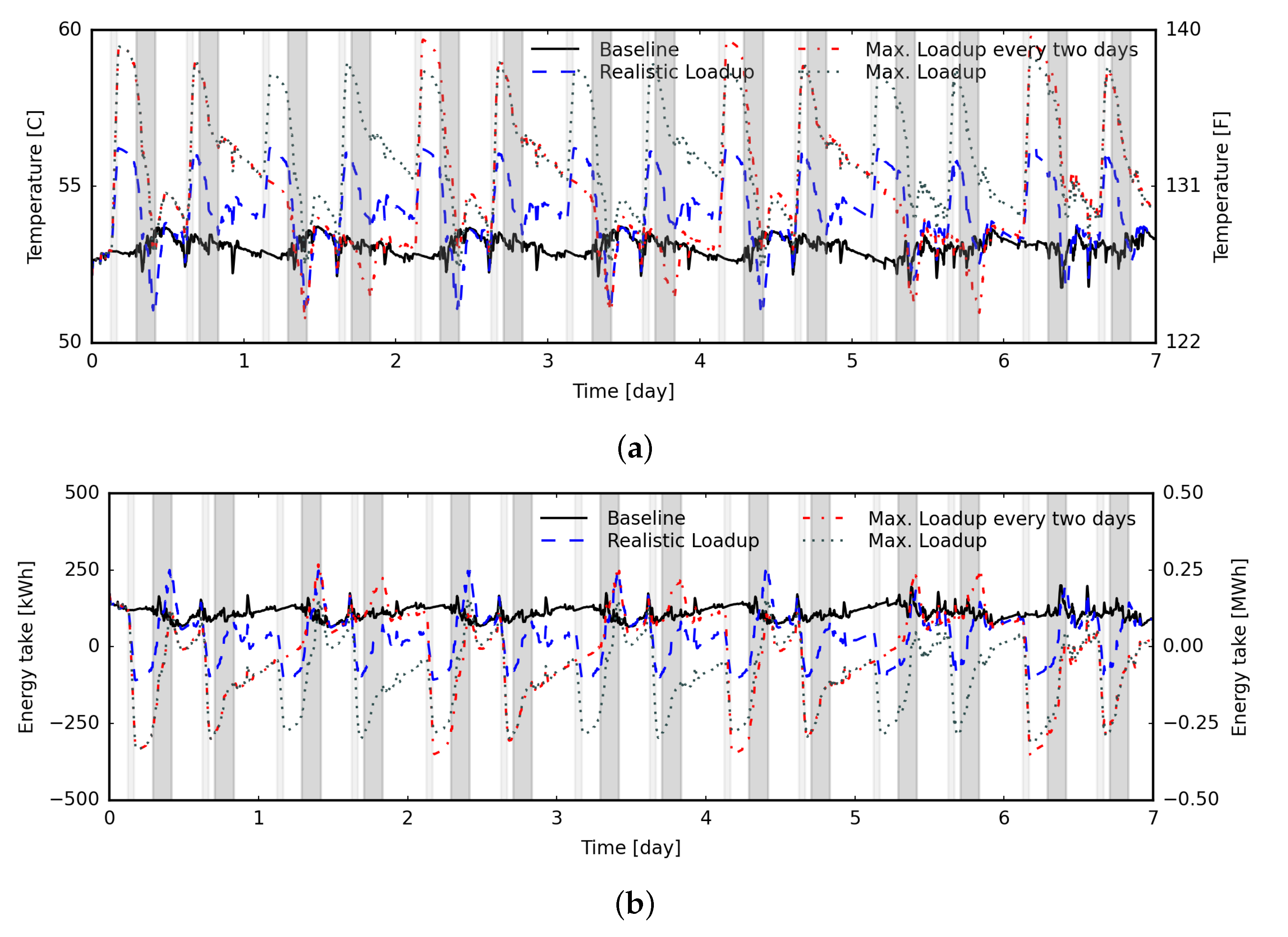
7. Long-Term EWH VPP Feasibility Case Study

To assess the capability of the controls across a long-term period, the IEEE 123 bus system was modified to co-simulate five distinct work-day and two weekend-day time series profiles for residential load and HWD from experimental datasets, as described in Section 4. The simulation starts on a Wednesday to encompass the affects of the weekend in the middle of the week. Within this setup, a representative synthetic community is employed with randomness from human behavior included.
The no load-up case was dropped and replaced with a maximum load-up every two days to represent a program where users have agreed to more comfort violations in return for an incentive. The control window times were kept constant from the daily case at time windows of 3–4, 15–16 and 7–10, 17–20 for load-up and shed, respectively. Aggregate power, EWH power, temperature, and energy take are visualized in Figure 16. Sequential controls were used for each DR window to prevent large spikes in power. Through out the simulation week, 194.2, 172.8, and 167.6 MWh of energy were shed during times of high congestion and strain on the distribution system in the max load-up, max load-up every two days, and realistic load-up cases, respectively. This represented 75, 66, and 64% of the EWH load and 23, 21, and 20% of the total load during shed windows.
The realistic load-up case returns the temperature to be equal to the baseline case, representing sustainability of the controls in terms of comfort and ability to meet the HWD demand while providing grid services (Figure 17). The maximum load-up and maximum load-up every two days cases leave the average temperature higher than the baseline but within 2 °C. The total energy used to heat the water increases with the controls by 0.4, 1.3, and 1.6%, which is a low amount justified by grid operation improvements from substantial load shifting. The load-up periods that drive this energy increase could be aligned with times of renewable energy generation as well.
Employing energy take to determine the heating element status of the EWH is successful at maintaining acceptable tank temperatures and providing grid services. Using the benchmark system and procedure within this work, further development of the timing of controls is possible, including formal optimization of load-up and shed times to reduce cost to the utility or increase renewable energy generation. The framework allows for long-term control studies for smart controls while EWH modules opt into the shed period based on internal tank temperature calculations.

8. Discussion

Two scenarios of CVR across the VPP, including three cases each, were simulated from with 1.05 to 0.90 p.u. voltages levels. The potential for power shifting at the aggregated level and energy savings were not found in these studies on a representative distribution system due to constant thermal energy requirements to maintain temperature comfort limits. The aggregate power was also not reduced as the diversity in heating times across the community was reduced as individual EWHs took longer durations to heat with lower voltage. Further studies with CVR for particular appliances would be more impactful with loads that do not require constant energy to maintain comfort limits and user expectations.

8.1. Sequential Control Development

The sequential controls proposed in this paper required a management system be in place to coordinate the controls. The assumption in this work is that each home is equipped with a smart EWH to receive signals for the controls. The energy management system would need to select homes to be placed into a batch and select the order of the batches to be deployed. Both of these decisions could be decided through optimization to minimize impact on the distribution system.
Additionally, the size of batches and the energy usage limits could be optimized to improve the controls. In this section, the effects of adjusting the batch size, spacing, and energy take limits are assessed for their impacts on the benefits of sequential controls. In Figure 18a, three cases with varied energy usage limits are compared. The batch size of 24 houses and 4 min deployment time is maintained from the VPP scenarios in previous sections. The more thermal energy stored in the tank during load-up, the higher the spike in power and strain on the distribution system from the controls could be. For example, the Lim. −4000 Wh case is close to the true maximum allowed energy usage corresponding to 165 °F, results in significantly higher load-up spikes over 1500 kW even with the sequential controls. To reach this high energy take limit, Q T , m a x ( t , H W D ) , the EWHs must remain ON for over an hour, which means no EWH turn OFF before the one hour load-up period is complete and longer control periods would be necessary to spread out the additional spike. This control pattern with more extreme controls may be useful with low batch size across an entire night and utilities would have to gauge consumer adoption and incentive rates.
In Figure 18b, the energy usage limits were returned to Table 1 maximum load-up case, and the load-up period in the morning was increased from one hour to six hours. The batch size and deployment time are varied in three cases, 1 min 1 house, 8 min 40 houses, and 70 min 70 houses. Overall, the smaller the batch size, the lower and more constant the increase in demand during load-up periods would be. The batch size needs to be balanced with the length of the load-up period and the deployment time. For example, in the 1 min 1 house case, where a signal is sent to a house every minute, a low constant power draw is seen in the load-up period. This would be an ideal case except the response speed in this case was too slow to reduce the power during shed, so two sets of batch sizes and deployment spacing may be necessary for load-up and shed periods.
For the second case with 40 houses deployed every 8 min, all houses are phased-in within a shorter period of 3 h. The load-up power was higher than the baseline peak load and was inconsistent as houses finished heating in ∼5 min before others were deployed. In a community with different EWH types, it would be more difficult to select a deployment speed with out this effect. The 70 houses per 70 min case was included to show a deployment time and batch size that were not aligned as all houses finish before the next fleet, resulting in evenly spaced spikes every hour, which would be more difficult for the utility to meet. Further investigation of the controls per utilization purpose would be needed with targeted objectives and constraints for distribution system and utility. The concept behind the sequential smart controls has been demonstrated to highlight the potential for future development.

8.2. Large-Scale Energy Storage and Global Applications

The CTA-2045 based VPP simulations in this paper indicated that a common appliance in homes across the globe, the EWH, may be used to improve resiliency of the grid system without affecting comfort standards. Across the globe, EWH are projected to increase from a global market value of USD 23 to 38 billion with growth drivers in North and Latin America, Europe, Asia Pacific, and MEA [41], and, thus, are an excellent candidate for global VPP control development for use of thermal storage. By design, the CTA-2045 Standard was selected for the simulations because it is intended to facilitate interoperable VPP controls in large-scale deployment across appliances from different manufacturers as found in the U.S. and around the world. As part of the CTA-2045 industry standard, a modular communications interface is defined to streamline communication methods and formatting so that any demand response system may connect to any type of residential appliance.
The widely compatible RS-485 serial communication method is specified in a physical communications module that attaches to the appliance itself, and serial opcodes are also defined for the VPP commands to “load-up” the energy and “shed” to decrease the energy stored. Then, per the protocol, common methods, such as Wi-Fi, ZigBee, etc., may be used for secure data transport to and from any energy management system. In this paper, the VPP simulations follow these protocol definitions and serve to represent the benefits of the interoperable communications in communities with high user participation to motivate further large-scale physical adoption.
For example, in the case studies on the IEEE 123 bus system, the peak power was reduced by up to 23% at the power system level when the EWHs participated in the VPP operation. The proposed sequential deployment prevented many EWHs from being turned ON at the same time during pre-heating or after the controls. Up to 78% of EWH energy in shed periods was shifted while maintaining the water temperature on this benchmark distribution system. The co-simulation framework developed to simulate the CTA-2045 controls, EWH responses, and residential load on the distribution system is compatible with other larger systems, such as the IEEE 8500 node test feeder. The testbed is object oriented and the initialization of different distribution systems in OpenDSS in the U.S. or globally could be used to assess the benefits of the VPP from the EWH energy storage formulation and controls before infrastructure investment on the CTA-2045 physical modules and energy management system.

9. Conclusions

The modified single node model of an electric water heater (EWH) proposed in the paper provides ultra-fast results for the water temperature and energy storage estimates supporting large-scale simulations. Based on the model, a methodology for conservation voltage reduction (CVR) and smart controls was applied to a community of EWHs operating as a virtual power plant (VPP), and the impacts on the power system level were evaluated. The capability of the VPP to shift peak demand while considering user comfort was quantified on the benchmark IEEE 123 bus feeder, which was modified with experimental residential load from a large field demonstration and hot water draw profiles from CBECC-RES national survey. The CVR was tested in EWHs from 1.05 p.u. to 0.90 p.u. and results show that reduced power, which was caused by reduced voltage, prolonged the heating process of individual EWHs, leaving more EWHs operating during peak times. As a consequence, the CVR did not reduce the aggregate power consistently throughout the duration of the controlled event, nor did it reduce the daily energy demand.

Author Contributions

Conceptualization, R.E.A., H.G., T.R., B.B. and D.M.I.; methodology, R.E.A. and H.G.; software, R.E.A. and H.G.; validation, R.E.A., H.G., T.R., B.B. and D.M.I.; formal analysis, R.E.A.; resources, H.G., T.R. and B.B.; writing—original draft preparation, R.E.A. and H.G.; writing—review and editing, H.G., T.R., B.B. and D.M.I.; visualization, R.E.A.; supervision, D.M.I. All authors have read and agreed to the published version of the manuscript.

Funding

This material is based upon work supported by the National Science Foundation Graduate Research Fellowship under Grant No. #1839289. Any opinion, findings, and conclusions or recommendations expressed in this material are those of the authors and do not necessarily reflect the views of the National Science Foundation.

Acknowledgments

The support received by Rosemary E. Alden through a National Science Foundation (NSF) Graduate Research Fellowship under Award No. #1839289 is gratefully acknowledged. The support of the A.O. Smith Corporation and of the University of Kentucky L. Stanley Pigman Chair in Power endowment is also gratefully acknowledged.

Conflicts of Interest

The authors declare no conflict of interest.

References

  1. Electricity in the United States Is Produced (Generated) with Diverse Energy Sources and Technologies. Technical Report, USA Energy Information Administration (EIA). Available online: https://www.eia.gov/energyexplained/electricity/electricity-in-the-us.php#:~:text=Most%20electricity%20is%20generated%20with%20steam%20turbines%20using,largest%20source%E2%80%94about%2038%25%E2%80%94of%20U.S.%20electricity%20generation%20in%202021 (accessed on 6 June 2023).
  2. Du, Z.; Liu, G.; Huang, X.; Xiao, T.; Yang, X.; He, Y.L. Numerical Studies on a Fin-foam Composite Structure Towards Improving Melting Phase Change. Int. J. Heat Mass Transf. 2023, 208, 124076. [Google Scholar] [CrossRef]
  3. Gong, H.; Rallabandi, V.; McIntyre, M.L.; Hossain, E.; Ionel, D.M. Peak Reduction and Long Term Load Forecasting for Large Residential Communities Including Smart Homes With Energy Storage. IEEE Access 2021, 9, 19345–19355. [Google Scholar] [CrossRef]
  4. Gómez, M.; Collazo, J.; Porteiro, J.; Míguez, J. Numerical Study of the Thermal Behaviour of a Water Heater Tank with a Corrugated Coil. Int. J. Heat Mass Transf. 2018, 122, 574–586. [Google Scholar] [CrossRef]
  5. Han, F.; Feng, D.; Xin, P.; Wang, W. Thermo-hydraulic Characteristics of Thermal Interface Induced by Natural Convection in Water Tank with Internal Heat Source. Int. J. Heat Mass Transf. 2023, 211, 124212. [Google Scholar] [CrossRef]
  6. CTA. CTA Standard: Modular Communications Interface for Energy Management; Technical Report; Consumer Technology Association (CTA): Arlington, VA, USA, 2020. [Google Scholar]
  7. Larson, B.; Kvaltine, N. Laboratory Assessment of Demand Response Characteristics of Two CO2 Heat Pump Water Heaters; Ecotope Inc.: Seattle, WA, USA, 2015. [Google Scholar]
  8. Liu, Q.; Bao, Y. Scheduling and Control of Massive Electric Water Heaters Based on Equivalent Energy Storage Model. In Proceedings of the 2021 IEEE 5th Conference on Energy Internet and Energy System Integration (EI2), Taiyuan, China, 22–24 October 2021; pp. 1928–1933. [Google Scholar] [CrossRef]
  9. IEEE PES Test Feeder: 123-BUS Feeder. Available online: https://cmte.ieee.org/pes-testfeeders/resources/ (accessed on 6 June 2023).
  10. Bandyopadhyay, A.; Conger, J.P.; Webber, M.E. Energetic Potential for Demand Response in Detached Single Family Homes in Austin, TX. In Proceedings of the 2019 IEEE Texas Power and Energy Conference (TPEC), College Station, TX, USA, 7–8 February 2019; pp. 1–6. [Google Scholar] [CrossRef]
  11. Abbas, A.O.; Chowdhury, B.H. A Stochastic Optimization Framework for Realizing Combined Value Streams From Customer-Side Resources. IEEE Trans. Smart Grid 2022, 13, 1139–1150. [Google Scholar] [CrossRef]
  12. Maguire, J.; Fang, X.; Wilson, E. Comparison of Advanced Residential Water Heating Technologies in the United States; Technical Report; National Renewable Energy Lab. (NREL): Golden, CO, USA, 2013. [Google Scholar]
  13. Mukherjee, M.; Bhattarai, B.; Hanif, S.; Pratt, R. Electric Water Heaters for Transactive Systems: Model Evaluations and Performance Quantification. IEEE Trans. Ind. Inform. 2022, 18, 5783–5794. [Google Scholar] [CrossRef]
  14. Porteiro, R.; Chavat, J.; Nesmachnow, S. A Thermal Discomfort Index for Demand Response Control in Residential Water Heaters. Appl. Sci. 2021, 11, 48. [Google Scholar] [CrossRef]
  15. Obi, M.; Metzger, C.; Mayhorn, E.; Ashley, T.; Hunt, W. Nontargeted vs. Targeted vs. Smart Load Shifting Using Heat Pump Water Heaters. Energies 2021, 14, 7574. [Google Scholar] [CrossRef]
  16. Maguire, J.; Roberts, D. Deriving Simulation Parameters for Storage-Type Water Heaters Using Ratings Data Produced from the Uniform Energy Factor Test Procedure; Technical Report; National Renewable Energy Lab. (NREL): Golden, CO, USA, 2021. [Google Scholar]
  17. Ritchie, M.J.; Engelbrecht, J.A.A.; Booysen, M.J. Centrally Adapted Optimal Control of Multiple Electric Water Heaters. Energies 2022, 15, 1521. [Google Scholar] [CrossRef]
  18. Amasyali, K.; Munk, J.; Kurte, K.; Kuruganti, T.; Zandi, H. Deep Reinforcement Learning for Autonomous Water Heater Control. Buildings 2021, 11, 548. [Google Scholar] [CrossRef]
  19. Moradzadeh, M.; Abdelaziz, M. Optimal Demand Control of Electric Water Heaters to Accommodate the Integration of Plug-in Electric Vehicles in Residential Distribution Networks. In Proceedings of the 2020 IEEE Canadian Conference on Electrical and Computer Engineering (CCECE), London, ON, Canada, 30 August–2 September 2020; pp. 1–6. [Google Scholar] [CrossRef]
  20. Moradzadeh, M.; Abdelaziz, M. Reducing the Loss of Life of Distribution Transformers Affected by Plug-In Electric Vehicles Using Electric Water Heaters. In Proceedings of the 2019 IEEE Canadian Conference of Electrical and Computer Engineering (CCECE), Edmonton, AB, Canada, 5–8 May 2019; pp. 1–5. [Google Scholar] [CrossRef]
  21. Ritchie, M.J.; Engelbrecht, J.A.; Booysen, M.J. Practically-Achievable Energy Savings with the Optimal Control of Stratified Water Heaters with Predicted Usage. Energies 2021, 14, 1963. [Google Scholar] [CrossRef]
  22. CTA-2045 Water Heater Demonstration Report including a Business Case for CTA-2045 Market Transformation; Technical Report; BPA Technology Innovation Project 336; Northwest Energy Efficiency Alliance: Portland, OR, USA, 2018.
  23. Gong, H.; Jones, E.S.; Jakaria, A.H.M.; Huque, A.; Renjit, A.; Ionel, D.M. Large-Scale Modeling and DR Control of Electric Water Heaters With Energy Star and CTA-2045 Control Types in Distribution Power Systems. IEEE Trans. Ind. Appl. 2022, 58, 5136–5147. [Google Scholar] [CrossRef]
  24. Wang, Z.; Begovic, M.; Wang, J. Analysis of Conservation Voltage Reduction Effects Based on Multistage SVR and Stochastic Process. In Proceedings of the 2014 IEEE PES General Meeting Conference & Exposition, National Harbor, MD, USA, 27–31 July 2014; p. 1. [Google Scholar] [CrossRef]
  25. Wang, Z.; Wang, J. Time-Varying Stochastic Assessment of Conservation Voltage Reduction Based on Load Modeling. IEEE Trans. Power Syst. 2014, 29, 2321–2328. [Google Scholar] [CrossRef]
  26. Wang, Z.; Wang, J. Review on Implementation and Assessment of Conservation Voltage Reduction. IEEE Trans. Power Syst. 2014, 29, 1306–1315. [Google Scholar] [CrossRef]
  27. Schneider, K.P.; Fuller, J.C.; Tuffner, F.K.; Singh, R. Evaluation of Conservation Voltage Reduction (CVR) on a National Level; Technical Report; Pacific Northwest National Lab. (PNNL): Richland, WA, USA, 2010. [Google Scholar]
  28. Jones, E.S.; Jewell, N.; Liao, Y.; Ionel, D.M. Optimal Capacitor Placement and Rating for Large-Scale Utility Power Distribution Systems Employing Load-Tap-Changing Transformer Control. IEEE Access 2023, 11, 19324–19338. [Google Scholar] [CrossRef]
  29. McNamara, M.; Feng, D.; Pettit, T.; Lawlor, D. Conservation Voltage Reduction/Volt Var Optimization EM&V Practices; Technical Report; Climate Protection Partnerships Division in EPA’s Office of Atmospheric Programs, DNV GL, The Cadmus Group: Waltham, MA, USA, 2017. [Google Scholar]
  30. Zhao, J.; Wang, Z.; Wang, J. Robust Time-Varying Load Modeling for Conservation Voltage Reduction Assessment. IEEE Trans. Smart Grid 2018, 9, 3304–3312. [Google Scholar] [CrossRef]
  31. Singh, S.; Babu, P.; Singh, S.P. Impact of Combined Operation of CVR and Energy Storage System in Distribution Grid. In Proceedings of the 2018 20th National Power Systems Conference (NPSC), Tiruchirappalli, India, 14–16 December 2018; pp. 1–6. [Google Scholar] [CrossRef]
  32. Ellens, W.; Berry, A.; West, S. A Quantification of the Energy Savings by Conservation Voltage Reduction. In Proceedings of the 2012 IEEE International Conference on Power System Technology (POWERCON), Auckland, New Zealand, 30 October–2 November 2012; pp. 1–6. [Google Scholar] [CrossRef]
  33. Jia, R.; Nehrir, M.H.; Pierre, D.A. Voltage Control of Aggregate Electric Water Heater Load for Distribution System Peak Load Shaving Using Field Data. In Proceedings of the 2007 39th North American Power Symposium, Las Cruces, NM, USA, 30 September–2 October 2007; pp. 492–497. [Google Scholar] [CrossRef]
  34. Pinney, D. Costs and Benefits of Conservation Voltage Reduction; National Rural Cooperative Association: Arlington, VA, USA, 2013. [Google Scholar]
  35. Lovas, T.; Pinney, D.; Miller, C. Costs and Benefits of Conservation Voltage Reduction. CVR Warrants Careful Examination; Technical Report DE-0E0000222; Cooperative Research Network, National Rural Electric Cooperative Association (NERCA), Department of Energy (DOE): Washington, DC, USA, 2014. [Google Scholar]
  36. Ritchie, M.; Engelbrecht, J.; Booysen, M. Impact of Node Count on Energy-optimal Control of Stratified Vertical Water Heaters in Smart Grid Applications. In Proceedings of the 2022 IEEE PES/IAS PowerAfrica, Kigali, Rwanda, 22–26 August 2022; pp. 1–5. [Google Scholar] [CrossRef]
  37. Xu, Z.; Diao, R.; Lu, S.; Lian, J.; Zhang, Y. Modeling of Electric Water Heaters for Demand Response: A Baseline PDE Model. IEEE Trans. Smart Grid 2014, 5, 2203–2210. [Google Scholar] [CrossRef]
  38. Thomas, C. Performance Test Results: CTA-2045 Water Heater; Technical Report 3002011760; Electric Power Research Institute (EPRI): Palo Alto, CA, USA, 2017. [Google Scholar]
  39. TVA Smart Community. Available online: https://www.tva.com/environment/environmental-stewardship/epa-mitigation-projects/smart-communities (accessed on 6 June 2023).
  40. CBECC-Res Compliance Software Project. Available online: http://www.bwilcox.com/BEES/cbecc2019.html (accessed on 6 June 2023).
  41. GMI. Electric Water Heater Market Size, by Product (Instant, Storage), by Application (Residential, Commercial [College/University, Office, Government/Military]), by Capacity, COVID-19 Impact Analysis & Global Forecast, 2022–2030; Technical Report GMI680; Global Market Insights (GMI): Selbyville, DA, USA, 2022. [Google Scholar]
Figure 1. Normal (a) and “load-up” (b) numerical simulation of an EWH satisfactorily modeled based on hot water draw profiles from the CTA-2045 experimental testing by EPRI and NREL [38]. The proposed modified single node model is employed with Energy Star-based heating element controls through the “energy take”.
Energies 16 04747 g001
Figure 2. The proposed single node EWH model for large-sale simulation with electric power distribution systems has been integrated into a testbed framework for the CVR and CTA-2045 based VPP simulations.
Energies 16 04747 g002
Figure 3. Modified IEEE 123 bus testfeeder populated with filed measured residential loads from the SET project and EWH power from model-in-the-loop objects, (a). Example 1R1C thermal model results for EWH power based on CBECC Res Project hot water draw (HWD) profile is illustrated. The proposed heated tank volume assumption of an η of 0.9 based on typical thermal areas with respect to the heating element, (b).
Energies 16 04747 g003
Figure 4. Individual home’s power, energy take (a), and temperature (b) in each case. The power magnitude and speed the energy take changes with the voltage. The EWH remains on for longer time the lower the power drops because the same amount of energy is required to heat the water to the set temperature.
Energies 16 04747 g004
Figure 5. Aggregate active power on the IEEE 123 bus test-feeder at the main feeder (a) and total EWH power from the community (b) has little affect in three CVR cases, where the BTM voltage of the EWHs was changed to 1.05, 0.95, or 0.90 p.u. All DR periods in this paper are visualized by grey shading and green color was assigned to Vp.u.0.95 case as this is the lowest voltage within typical allowed range in the U.S.
Energies 16 04747 g005
Figure 6. Enlarged CVR periods in the morning (a) and afternoon (b) shows that the CVR completed on individual EWH does not always translate to power reduction at an aggregate level as longer heating times at lower powers may cause more EWH to be on at a time.
Energies 16 04747 g006
Figure 7. The hour surrounding the peak power in the morning (a) and evening (b). The percentage of additional houses operating in comparison to the Vp.u.1.0 case shown by discrete points corresponds to times when the aggregate power does not reduce. An example time when CVR does reduce the power occurs at 9:15 a.m. when the number of houses operating is not increased.
Energies 16 04747 g007
Figure 8. Morning (a) and afternoon (b) CVR simulation repeated with higher thermal resistivity, 1500 °C/kW, and lower rated power, 4.5 kW, to show that many parameters affect the success of CVR at the aggregate level. EWH peak load changes of −9.99, −5.00, and 3.98% in the 0.90, 0.95, and 1.05 V p.u. cases. Overall, power reductions are not consistent across the DR period like the previous scenario.
Energies 16 04747 g008
Figure 9. A closer look at the hour surrounding the peak in the morning (a) and evening (b) shows that while a reduction happens at 9:20 a.m. when the load is the highest, it is not consistent across the time window. It also is affected an increased percentage of EWHs heating per minute, thus, mitigating the affects of CVR at the community level.
Energies 16 04747 g009
Figure 10. The number of minutes the EWHs spend heating across the day reduces between p.u. cases as the voltage increases as expected. On average, it is also lower for the 5.5 kW simulation (top) than the 4.5 kW simulation (bottom). For example, in the Vp.u.0.95 case heating for 51 and 62 min, respectively, as visualized by the green lines.
Energies 16 04747 g010
Figure 11. The CTA-2045 “load-up” case resulted in large spikes of power of more than twice the typical peak load at the main feeder and in total EWH power, (a,b), respectively. Large spikes are also present the following shed periods. The average energy take, (c), and internal tank temperature, (d), of the load-up and max load-up cases returns within 4 °C, and the temperature of the water tanks do not violate comfort limits.
Energies 16 04747 g011
Figure 12. The sequential controls reduce power spikes by three times at the main feeder and in the total EWH power, (a,b), respectively. They do not affect the temperature, (c), or energy usage, (d). During shed times, the EWH power is curtailed and the sequential controls stop swing back spikes following the event.
Energies 16 04747 g012
Figure 13. The status of the individual EWHs are visualized, (a), and the individual temperatures in the tanks are depicted in a boxplot form based on the distribution with outliers shown as red stars, (b). All EWH operated during the load-up periods and operation was postponed during shed events. Following the shed, the EWH turn ON with the same spacing as the load-up, successfully mitigating a bounce back spike.
Energies 16 04747 g013
Figure 14. The energy take per EWH (a) and bus voltages (b) across the community are visualized as boxplots based on the distribution at that 30 min increments. The maximum energy take, Q T , m a x ( t , H W D ) , per Table 1 is depicted the solid blue line, this indicates that outliers above the limit in shed periods required heating. No voltage violations were found across the buses in the distribution system.
Energies 16 04747 g014
Figure 15. An enlarged visualization of the voltages during the CTA-2045 controls. No violations found as a result of the controls.
Energies 16 04747 g015
Figure 16. The CTA-2045 controls applied to a week long case simulation period starting on a Wednesday in the summer. The aggregate total (a) and EWH power (b) is consistent across days of the work week, and load is successfully reduced during shed times.
Energies 16 04747 g016
Figure 17. The VPP average temperature (a) in the tank recovers following the controls over the course of the week and average energy take is visualized (b). Little variation occurs between weekend and work-day effects.
Energies 16 04747 g017
Figure 18. Three load-up cases are compared to show that the energy take limits directly affect the magnitude of the power spikes (a). Three more examples are shown (b) to compare effects of the batch size and spacing period of signals, and a longer control window is required for more spaced out controls.
Energies 16 04747 g018
Table 1. The three cases considered in this study for load shifting using CTA-2045 commands and Energy Star energy storage calculations.
CasesEventEnergy Take [Wh]Max Cap. [Wh]
(Thermal)
MinMax
BaselineNormal (Water
draw dependent)
0300: >= 1 GPM300
600: >=0.3 GPM600
900: <0.3 GPM900
No load-upShed100015001500
Realistic load-upload-up−300 *01800
Shed10001500
Max load-upload-up−1000 *02500
Shed10001500
* Temperatures higher than the set-point are represented by a negative sign, specifically for a set-point of 125 °F, energy take values of −300 and −1000 correspond to internal tank temperatures of 128 and 133 °F.
Table 2. Energy over the simulation day for the EWHs shows minimal reduction in energy, i.e., less than the anticipated 1–4% of energy reductions from CVR [29].
CVR CaseAggregate EWH Energy [MWh]Average Individual EWH Energy [kWh]Daily Energy Reduction [%]CVR Factor [-]
V p.u. 1.051.6391.1390.04−0.008
V p.u. 1.001.6401.138- *- *
V p.u. 0.951.6381.1370.070.014
V p.u. 0.901.6431.140−0.18−0.018
* Base case that others are compared to for energy reduction.
Disclaimer/Publisher’s Note: The statements, opinions and data contained in all publications are solely those of the individual author(s) and contributor(s) and not of MDPI and/or the editor(s). MDPI and/or the editor(s) disclaim responsibility for any injury to people or property resulting from any ideas, methods, instructions or products referred to in the content.

