1. Introduction
Well production is aimed at finding the optimal production solution for each well to maximize the net present value (NPV) or production of hydrocarbons from a reservoir, which falls under the category of production optimization. The optimization process involves forecasting future production, and numerical simulators are often used for this purpose. However, individual simulation runs can be time-consuming, and complete optimization may demand numerous simulation iterations [
1]. Consequently, it is critical to devise efficient methodologies to address these challenges.
Currently, there are two main types of methods commonly used for well production: optimization algorithm-based methods and reinforcement learning (RL) methods. Among them, the optimization algorithm-based methods mainly include gradient-based methods and derivative-free methods. Gradient-based algorithms use gradient data to determine the search direction [
2,
3,
4,
5]. The mainstream gradient-based methods that have been used for production optimization problems are the adjoint gradient-based method [
6], the stochastic gradient method [
3], the synchronous perturbation stochastic approximation [
7], etc. These methods have been proven to be able to provide fast and accurate solutions for production optimization problems. However, these methods can only ensure finding locally optimal solutions. Therefore, there is a need for more efficient methods that can find globally optimal solutions. Alternatively, derivative-free algorithms do not require the explicit computation of derivatives, and therefore, offer better flexibility [
8,
9]. Representative algorithms are differential evolution (DE) [
10,
11], agent-assisted evolution algorithm (SAEA) [
12,
13,
14,
15,
16,
17,
18,
19], particle swarm optimization (PSO) [
20], etc. These methods have been widely used in various optimization tasks and have shown excellent global search capability. However, this method requires a large number of simulations, has low computational efficiency, and is difficult to solve for high-dimensional problems, making it difficult to apply in this field. A drawback of optimization algorithm methods is that they are task-specific, lack memory, and need to restart for new tasks.
Recent studies have attempted to use RL algorithms to solve specific problems in production optimization, such as De Paola et al. using the DQN algorithm (De Paola et al., 2020), or Zhang et al. using the SAC algorithm for full life-cycle water drive production optimization [
21]. Although these studies have the capacity to markedly improve the final recovery in dynamic production optimization using RL, most of the RL models are learned and trained for specific reservoirs, and thus can only be used for the current reservoir; when applied to other reservoirs, they generally perform poorly. To address this limitation, recent work has begun to focus increasingly on using RL to solve generalized problems for different reservoir optimization models. For example, Miftakhov et al. proposed an end-to-end strategy optimization combined with pixel data to maximize the NPV of production processes [
22]. Additionally, Nasir et al. developed a standard reservoir template on which to train an RL model for field development plan (FDP) optimization; when applied to a real reservoir, the real reservoir is rescaled to the reservoir template, thereby solving scalable field development optimization problems [
23,
24]. Furthermore, a general control strategy framework based on deep reinforcement learning (DRL) was developed by Nasir and Durlofsky for closed-loop decision-making in subsurface flow environments [
25]. Here, the closed-loop reservoir management problem is expressed using a Markov decision process with partial observability and a proximal policy optimization algorithm is employed to solve the optimization problem. However, training the models requires significant computational effort, and the resulting generalized RL optimization models are not yet achieved.
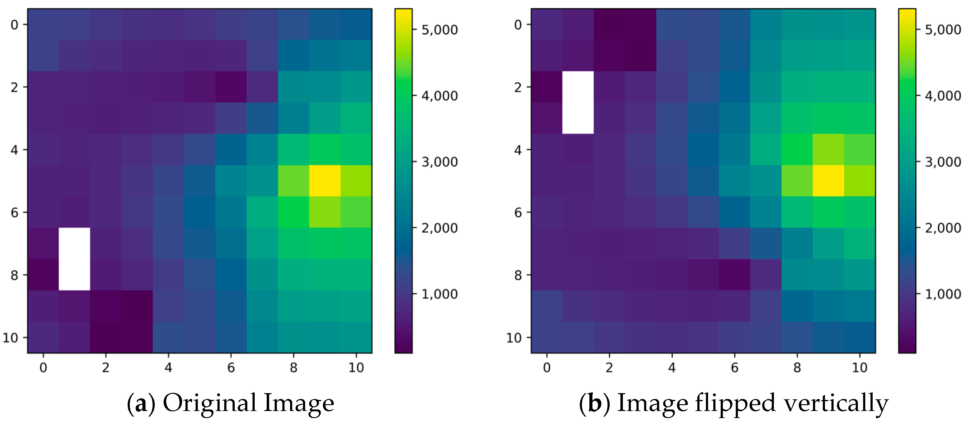
In this paper, we propose a new approach that utilizes convolutional neural networks (CNNs) and RL algorithms to optimize well production in reservoir engineering. Our approach involves dividing the reservoir into fundamental production units. Each unit comprises a group of wells with distinct geological and developmental characteristics. In the field of reservoir engineering, this type of production unit, which consists of a central well and its associated neighboring wells, is commonly referred to as a “well group”. By doing so, the sample size increases significantly, covering a broader range of characteristics and simplifying the model training process. Moreover, image enhancement techniques can be employed to further improve the coverage of the samples.
We present two frameworks for optimal control of the well workover regime. The first framework employs a CNN in deep learning, taking the well group as input and outputting the optimal working regime of the well group in terms of bottomhole pressure (BHP). The optimal production strategy is obtained through RL algorithms, which are then used to label the samples before training the algorithm. The second framework also uses CNN networks in deep learning but incorporates labels obtained from RL algorithms using well revenue (NPV) under a certain BHP as its sample label. We demonstrate the effectiveness of our approach through extensive experiments and analysis.
The following sections outline the structure of this paper.
Section 2 introduces the mathematical model for production optimization and describes the main processes of the two frameworks.
Section 3 outlines the main algorithms employed in this study.
Section 4 discusses the dataset used for the study. In
Section 5, we present a test case to illustrate the application of the proposed methods. Finally, we summarize the main conclusions of this study in
Section 6.
2. Production Optimization Problems and Solutions
2.1. Mathematical Model for Production Optimization
Production optimization seeks to achieve maximum financial gain or hydrocarbon production by adjusting the control strategy for each well [
26,
27].
Mathematically, the optimization problem for oil field development can be expressed as follows:
The objective function, denoted by , is to be optimized, and the decision vector defines the specific production strategy of the well. The space defines the range of values of the decision variables, while the vector defines the optimization constraints that must be satisfied.
In this study, the objective function to be optimized is the NPV of the production process. The formula for calculating NPV is as follows:
In Equation (2), and represent the total number of injection and production wells, respectively. used to indicate the total number of reservoir simulation steps, with in units of days being the length of the th time step, and in units of days being the cumulative time up to the th time step. denotes the oil revenue in USD/STB, which is set as 70 USD/STB in this paper; represents the cost of disposing of the produced water in USD/STB, which is 5 USD/STB in this paper; denotes the cost of injecting water in USD/STB, which is 5 USD/STB in this paper. denotes the annual discount rate, which is 0 in this paper. and represent the oil production rate and water production rate in STB/D of the th production well during the th time step, respectively; denotes the water-injection rate of the th injection well at the th time step (in STB/D).
In this study, the decision vector
is the BHP of the well, and the range of values X of the decision variables and the optimization constraints
are specified in
Section 3.1.
2.2. Algorithmic Framework for Oil Well Production Optimization
In this study, we propose two novel frameworks for developing a general model for regulating well production strategy. These frameworks differ from previous approaches that rely on iterative optimization-based algorithms to explore numerical simulators or use RL to train a proxy model for well Production. The specifics of these two frameworks are elaborated below.
2.2.1. Framework 1
Figure 1 illustrates Framework 1, which consists of three main steps that correspond to ①, ② and ③ on the right side of the figure. The first step involves the preparation of the sample set. We develop a personalized deep Q-network (DQN) algorithm and use it to conduct RL on the cropped well group sample. When a well group sample is inputted into the algorithm, the algorithm aims to maximize the NPV of that well group. It achieves this by evaluating the NPV of the recommended BHP through numerical simulation until the optimal BHP for the well group is obtained. Each inputted well group sample, along with the corresponding optimal BHP recommended by the personalized DQN algorithm, will be stored in the sample repository. By optimizing a large number of cropped well group samples using RL, we can generate a diverse sample set containing cropped well group samples with their corresponding optimal BHPs for numerous cases. The second step involves the training of the model. We build a CNN and train it using the aforementioned sample set. Finally, we obtain a CNN model. The third step involves the application of the model. The details of the personalized DQN algorithm are explained in
Section 3.1, the construction of the CNN network structure in
Section 3.2.1, and the preparation of well groups in
Section 4.
2.2.2. Framework 2
As shown in
Figure 2, Framework 2 is comprised of a three-step process, i.e., ①, ② and ③ in the figure. The first step is to construct a sample set that contains more development information: unlike Framework 1, which only records the well group and the optimal BHP recommended by the personalized DQN algorithm for each input, Framework 2 also saves the NPV corresponding to each BHP obtained by the personalized DQN algorithm. The second step is to train a CNN model that can predict development effects under different production strategies. First, we construct a CNN network that differs from the one in Framework 1. Then, we use the sample set to train the CNN network. The last step is to apply the CNN model to generate optimal production strategies. First, particle swarm optimization, an intelligent optimization algorithm, is utilized in this study to automatically generate a batch of production strategies and invoke the CNN model to quickly predict their development effects. Then, we pass these development effects to PSO, which generates a new batch of production strategies based on them. By repeating this process, PSO eventually converges to the optimal production strategy. We will introduce PSO in
Section 3.3 and describe the structure of the CNN network in
Section 3.2.2.
3. Algorithms
3.1. Personalized DQN Algorithm
RL is a process of trying different actions and interactions through the environment in order to find the optimal strategy based on feedback from the environment. This approach can also be used to preserve experience. In the context of well workover optimization, RL can be applied by using the well group as the input, the BHP as the action, numerical simulation as the environment, and the NPV as the feedback. By doing so, optimal BHP or NPV labels can be added to subsequent well group samples.
As RL is not a specific algorithm, but rather a generic term for a class of algorithms, the choice of a suitable algorithm is necessary. The popular RL algorithms include DQN, Soft Actor-Critic, and Proximal Policy Optimization. In this study, the DQN algorithm was chosen to minimize computational stress on the computer.
In this paper, we investigate a single-step optimization problem for oil wells. However, the current DQN algorithm [
28] was originally designed for a multi-step time series problem. Therefore, we have made modifications to the algorithm to make it suitable for our research needs, resulting in the personalized DQN algorithm. Specifically, we have made two main modifications to the DQN algorithm: (1) we have modified the network structure, and (2) we have adjusted the mathematical expression used for calculating the value of the action.
Modification of network structure: In the original DQN algorithm process, a two-layer neural network is initialized, comprising the original neural network with parameters and the target neural network with parameters . However, the target neural network is designed to stabilize the training process of network optimization for multi-step time series problems, which is not necessary for our research. Therefore, we removed the target neural network from the personalized DQN algorithm to meet the requirements of our single-step optimization problem.
Modification of the mathematical expression for calculating the value size of an action: The reward of an action to be taken in RL is a measure of its value size and can be estimated using the expression given in Equation (3).
In Equation (3), is the reward value of the current action. is an estimate of the value of performing a future action in the state. is the discount rate, which discounts the value of the future action to the current node and takes a value between 0 and 1.
Since this paper studies a single-step optimization problem for oil wells, only one action is generated in each training, and there are no future actions. Thus, there is no need to estimate the value of future actions, so in Equation (3) should be removed. Consequently, Equation (3) becomes .
In conclusion, Algorithm 1 presents the pseudo-code of the personalized DQN algorithm that we designed for the single-step optimization problem of well parameters.
| Algorithm 1: Personalized DQN algorithm |
Initialize replay memory with capacity size ;
Initialize the action-value function with random parameters ;
For episode = 1, do:
Initialize sequence ( is the image) and preprocessed
sequence ;
With probability select a random action ,
Otherwise, select the largest value of action according to the
formula ;
Execute action in environment and observe reward and image ;
Let and obtain ;
Store an experience data in the replay memory ;
Randomly sample a batch of data from ;
Using to obtain ;
Updating the network parameters according to the gradient
descent algorithm;
End for
Output: model with parameter . |
3.2. Construction of CNN Networks
Since this study adopts two frameworks to optimize the oil well production strategies, and the CNN network structures required by these two frameworks differ significantly, two different CNN network structures need to be built. The detailed descriptions of these two CNN network structures are as follows.
3.2.1. Network Structure 1
The first network structure, referred to as Network Structure 1, is designed specifically for Framework 1, as shown in
Figure 3. Designing the architecture of neural networks does not have specific guidelines to follow [
29], as it requires customization based on the specific problem and empirical knowledge. In our study, we drew inspiration from a related research study [
21] that employed network structures and made adjustments to the framework based on the requirements of our research problem. As a result, we arrived at the architecture depicted in
Figure 3. This neural network comprises seven layers, including two convolutional layers, four hidden layers, and one output layer. The input to the network is the well group, and the output is the BHP recommended by the algorithm. Notably, the BHP values in the output layer are restricted to a range of −1 to 1 and are discretized into 21 discrete values, corresponding to the 21 neurons in the output layer. In this discretization scheme, 0 represents the default BHP value of the well group, while 1 and −1 represent the upper and lower BHP values of the well group, respectively. This approach aims to enhance the universality of the trained CNN network and to reduce the difficulty of training the algorithm.
3.2.2. Network Structure 2
Network Structure 2 is specifically designed for Framework 2, as illustrated in
Figure 4. The neural network consists of seven layers in total, with two inputs: the well group, which is connected to the convolutional layer, and the BHP of the well group, which is merged with the well samples after two convolutions to be inputted into the first fully connected layer. The output of the network is the NPV obtained by producing the well group at a given BHP. Based on the foundation of network structure 1, we have designed this network architecture by incorporating the unique features of Framework 2. Within a given well group, by incorporating BHP as an input, the CNN model can understand how different BHP values impact the NPV. The model learns to capture patterns and correlations between various BHP settings and their corresponding NPV outcomes. This enables the CNN model to predict the NPV based on the input well group and BHP values. It is important to note that we normalize the input BHP and restrict the NPV of the output layer to a range of 0 to 1. The closer the output value is to 1, the better the BHP. This is conducted to make the trained CNN network more generalizable.
3.3. PSO Algorithm
PSO is a method of evolutionary computation that was introduced by Dr. Eberhart and Dr. Kennedy in 1995 [
30] and originated from the study of bird flock predation behavior. Each individual in a flock can be treated as a particle, and the flock can be considered a particle swarm. The specific algorithmic procedure of the PSO can be referred to as presented in Marini F and Walczak B (2015) [
31].
In this subsection, the main parameters of the PSO algorithm are presented. In this study, the independent variable is the standardized BHP, the objective function is the CNN network model in Framework 2, and the fitness function is the NPV of the model’s output. The termination condition is that the algorithm iterates 50 times. The number of particles is set to 50. The maximum velocity of the particles is set to 0.5, and the inertia factor is set to 1.0. The search space for particles corresponds to the range of standardized BHP values, i.e., −1 to 1. The individual learning factor and social learning factor are both set to 2.
These settings aim to strike a balance between exploration and exploitation during the search and reduce the risk of converging to a suboptimal solution. By utilizing 50 particles, we can explore the solution space more comprehensively. Limiting the maximum velocity helps prevent particles from making sudden large jumps, thereby enhancing the convergence toward the optimal solution. The inertia factor of 1.0 ensures a balanced contribution from the previous velocity and acceleration, facilitating progressive search. Additionally, the individual and social learning factors of 2 promote information sharing and cooperation among particles, facilitating the exploration of promising regions within the search space. This helps prevent the algorithm from getting trapped in local optima by combining insights from personal and team experiences.
5. Case Study
5.1. Settings for Model Training and Validation
In the training phase, Training Set 1 and Training Set 2 were used to train the CNN networks in Framework 1 and Framework 2, respectively. The setting of hyperparameters, similar to the configuration of network structures, lacks a definitive guideline and requires consideration of specific research questions and experiential knowledge. Therefore, based on the particular problems within these two frameworks and common initial hyperparameter settings in CNNs, we have initially established the primary training parameters for the CNN networks under each framework, as presented in
Table 2. However, it is worth noting that the selection of hyperparameters is a dynamic process that may vary depending on the specific dataset, task, and experimental conditions. These initial settings serve as a starting point, and we will further refine and optimize them during subsequent hyperparameter tuning processes.
Two points need to be clarified before proceeding.
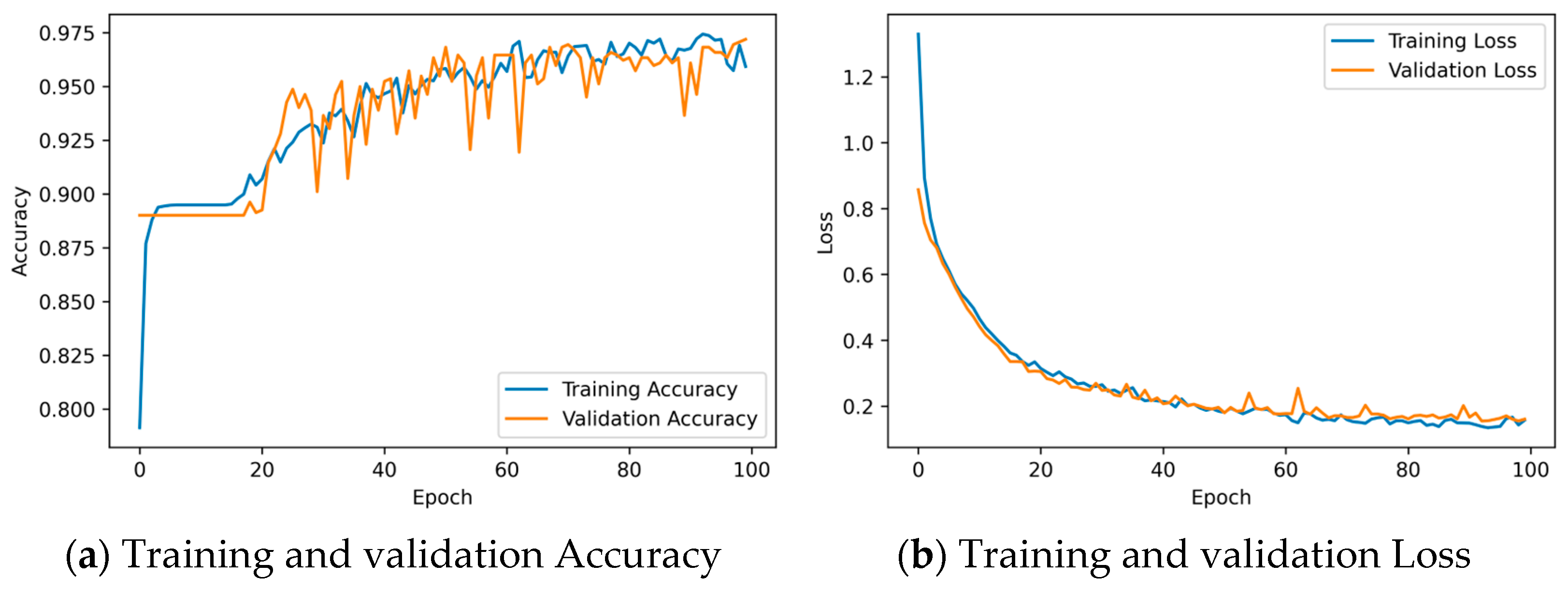
The CNN network structure in Framework 1 is designed for multi-classification problems, while the CNN network structure in Framework 2 is intended for regression problems. Therefore, the evaluation metrics for the CNN model in Framework 1 are accuracy and loss value, while the evaluation metric for the CNN model in Framework 2 is the loss value during training.
To prevent the trained model from underfitting or overfitting, we split both training set 1 and training set 2 into a training set and a test set with a ratio of 8:2. The model training result will show two curves in the image: one for the training set and one for the test set.
In the model validation phase, validation set 1 and validation set 2 are used to validate the effectiveness of the CNN model in Framework 1 and the PSO and CNN models in Framework 2, respectively. The model effectiveness is evaluated using the ratio of the number of optimal BHPs accurately recommended by the model to the total number of validation samples. It should be noted that the model validation is the overall effect of the two frameworks.
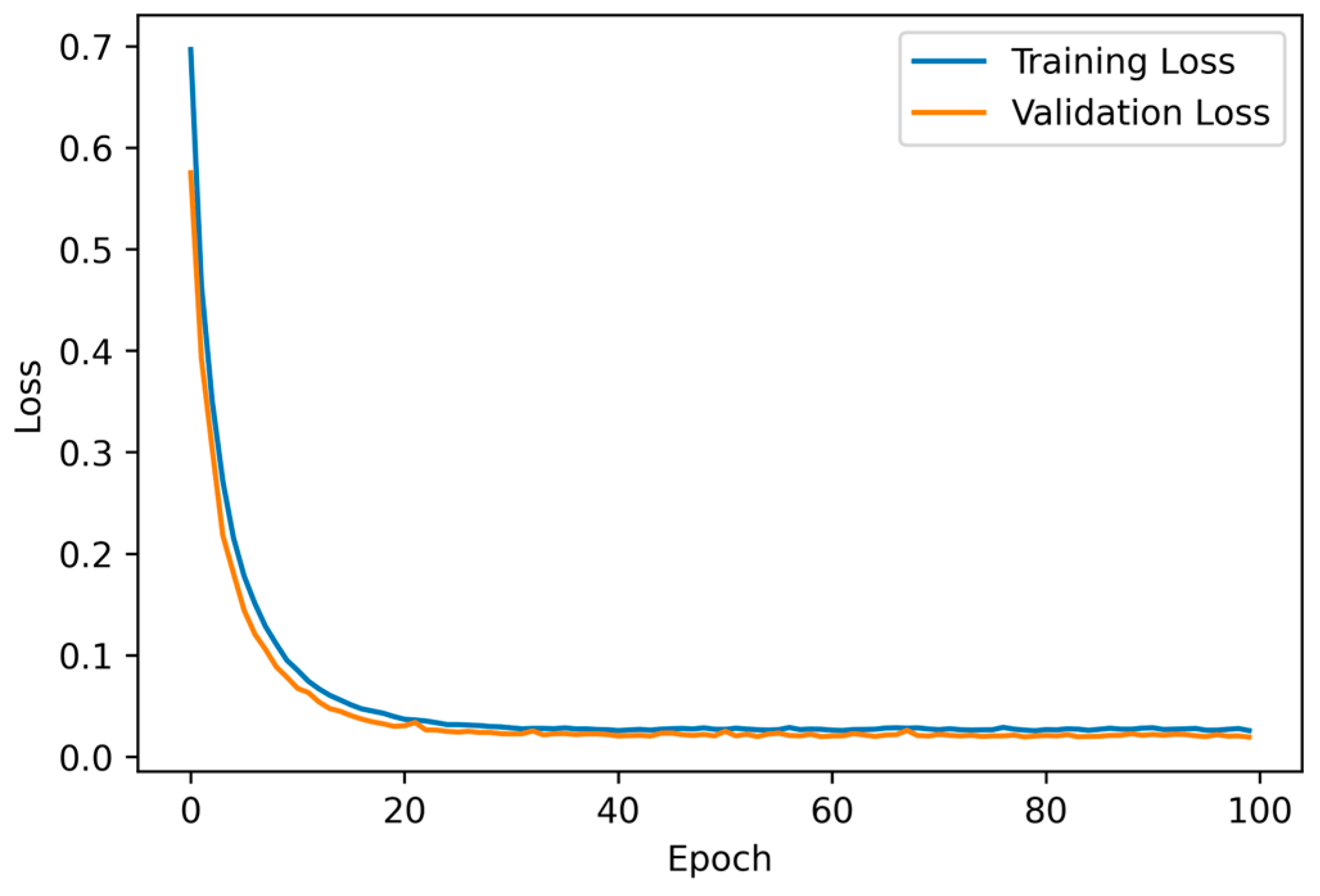
5.2. Model Training Results and Analysis
The results of training CNN networks in Framework 1 and Framework 2 are presented in
Figure 10 and
Figure 11, respectively.
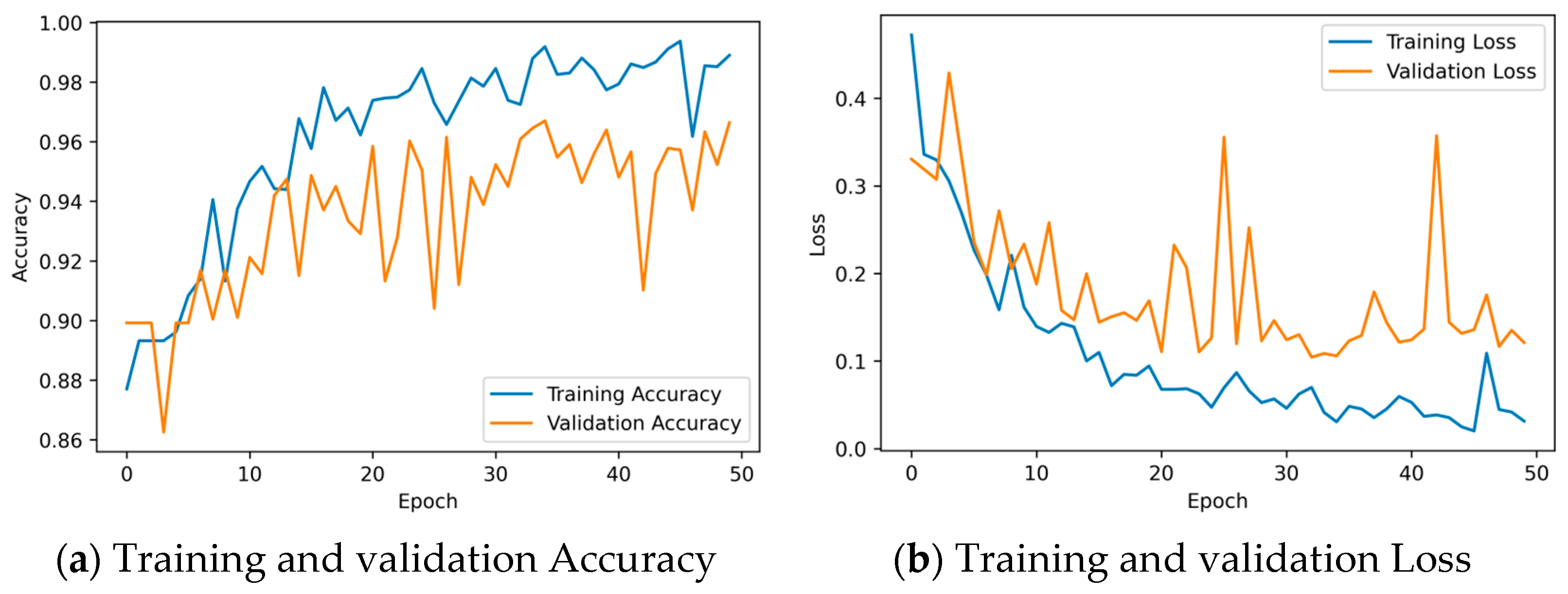
Figure 10a depicts the training accuracy of the CNN model in Framework 1, which is consistently above 98%, and the validation accuracy of the CNN model, which remains around 95%.
Figure 10b shows that both the training loss and validation loss of the CNN model decrease as the training progresses. The CNN model in Framework 1 was trained for 29 s. After the completion of training, the training set loss of the CNN model is approximately 0.15, and the validation set loss of the CNN model is around 0.05.
As shown in
Figure 11, the training and validation losses of the CNN model in Framework 2 decrease sharply at the beginning of training and then stabilize gradually. The model training time for this framework is 35 s, which is slightly longer than that of Framework 1. The training and validation losses of the CNN model are both below 0.01 at the end of training.
5.3. Model Validation Results and Analysis
This section mainly introduces the comparison results between the recommended optimal BHP values by Framework 1 and Framework 2 models and the actual optimal BHP values. The comparison results are shown in
Figure 12 and
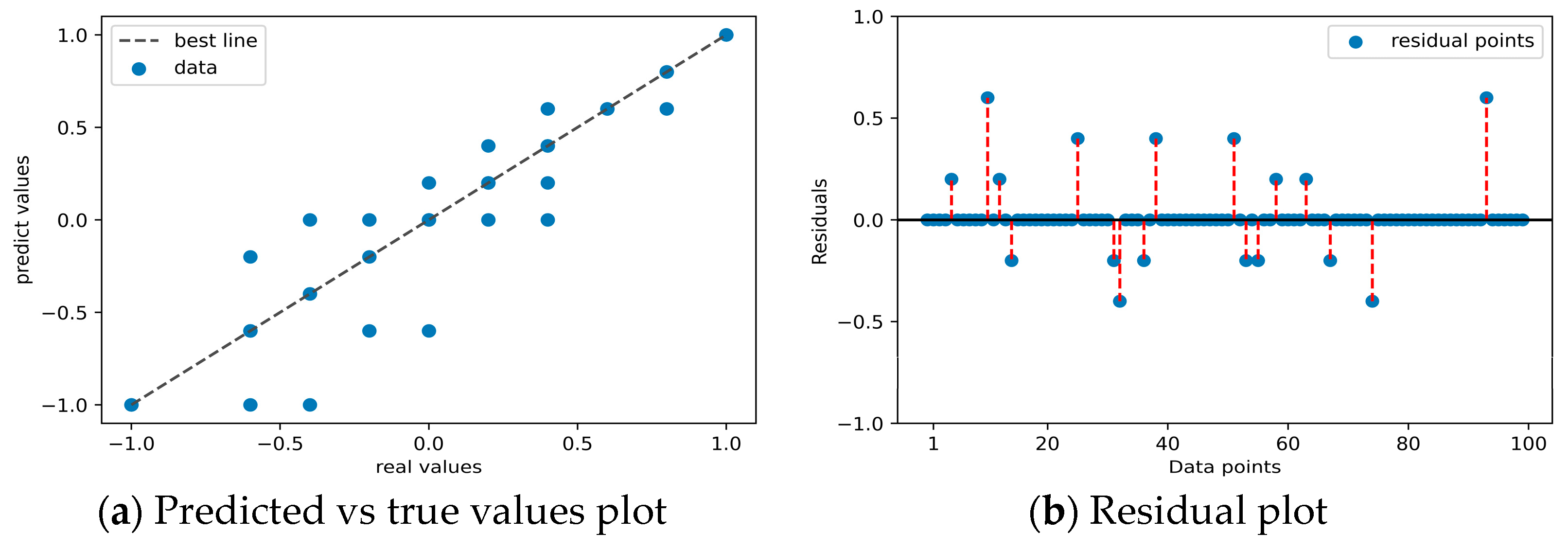
Figure 13, each of which has two subplots. In
Figure 12a and
Figure 13a, the x-axis corresponds to the actual optimal BHP value, and the y-axis corresponds to the model-predicted optimal BHP value. The closer the data points align with the diagonal line, the better the consistency between the predicted and actual values. Both
Figure 12b and
Figure 13b are residual plots, where the x-axis is the data point and the y-axis is the residual. There is a black line at the zero residual point, and the closer the residual points are to this line, the better the consistency between the predicted and actual values. Overall, both subplots convey the same information but in different forms. For clarity, only 100 comparison results are presented in the figure.
From
Figure 12, it can be seen that only a few data points deviate from the best line in
Figure 12a, and only a few residual points are not on the black line in
Figure 12b. This indicates that the recommended optimal BHP values by the Framework 1 model are highly consistent with the actual optimal BHP values. The optimal BHP output accuracy of this model can reach 82% of the entire validation set 1. On the other hand,
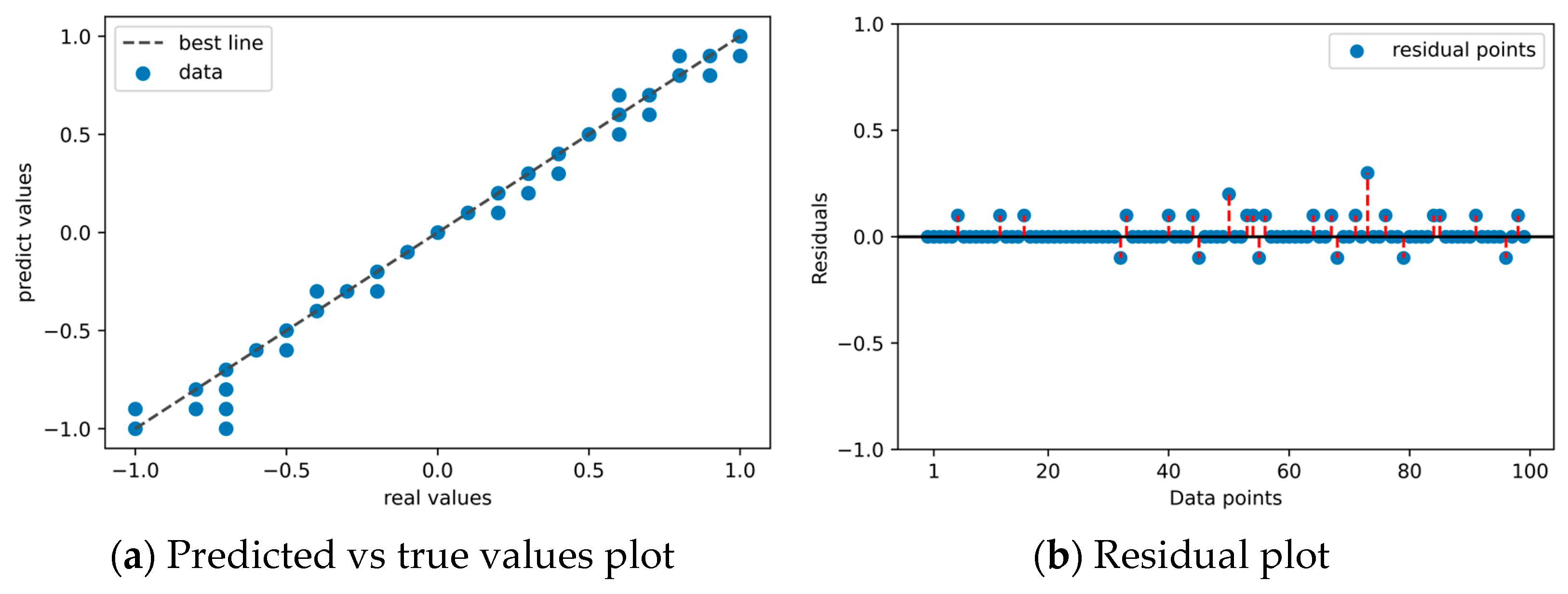
Figure 13 shows that the matching degree between the recommended optimal BHP values by the Framework 2 model and the actual optimal BHP values is lower than that of the former. However, most data points are still close to the best line. The optimal BHP output accuracy of this model is calculated to be 76% of the entire validation set 2.
After comparing the results of the two frameworks, it is evident that the model in Framework 1 outperforms the model in Framework 2 in terms of predicting the optimal BHP values. Additionally, it is worth emphasizing the superior computational efficiency exhibited by the model in Framework 1, as it completes the optimization task within 1 s, whereas the model in Framework 2 requires approximately 8 s. These findings underscore the advantages of the model in Framework 1, which achieves higher accuracy and faster execution, making it a more favorable choice for practical implementation.
To evaluate the performance of these two frameworks in the whole reservoir. Using both frameworks, we recommended BHP values for all well groups in the S1 model and had them produce according to these recommended BHP values across the entire reservoir.
The results revealed that Framework 1, with its recommended BHP values, generated a total profit of 11,522,300 USD for the entire reservoir production. On the other hand, Framework 2, with its recommended BHP values, resulted in a profit of 10,160,900 USD. In comparison, the baseline BHP value of 155 bar led to a loss of 701,533,900 USD. These findings clearly demonstrate the effectiveness of both Framework 1 and Framework 2 in optimizing the production of well groups, thereby significantly enhancing the economic performance of the entire reservoir. In terms of NPV, Framework 1 outperformed Framework 2, indicating its superior ability to maximize economic returns.
5.4. Comparison of Production Optimization Framework
This paper proposes two optimization frameworks for optimizing oil reservoir production strategies based on Convolutional Neural Networks (CNNs). In order to demonstrate the superiority of the proposed methods, they are compared with the PSO algorithm mentioned in the literature. Both the proposed frameworks and the PSO algorithm are applied to optimize a randomly selected set of 100 validation samples. The comparison is conducted based on the accuracy of the algorithms and the runtime per iteration. The accuracy is defined as the ratio of the number of wells for which the algorithms find the optimal BHP to the total number of wells requiring BHP optimization.
Regarding the parameter settings of the PSO algorithm in the context of this study, the main settings are as follows: the independent variable is BHP, and the fitness function is NPV obtained by the numerical simulation method. The termination condition is that the algorithm iterates 100 times. The number of particles is set to 100, the maximum particle velocity is set to 0.5, and the inertia factor is set to 1.0. The search space for particles corresponds to the range of BHP values, ranging from −1 to 1. Both the individual learning factor and the social learning factor are set to 2. The comparative results are summarized in
Table 3.
While PSO has proven to be effective in finding optimal solutions, the generated production strategies require a numerical reservoir simulator to evaluate their effectiveness, which is time-consuming and computationally intensive. In contrast, the proposed CNN-based frameworks have several advantages. Firstly, they decompose the reservoir into independent production units, reducing computational complexity and improving optimization efficiency. Secondly, image augmentation techniques are used to increase sample size and diversity, improving the accuracy and robustness of the proposed methods. Thirdly, using CNNs can efficiently and accurately predict optimal control strategies.
Experimental results show that the proposed frameworks outperform PSO-based methods in terms of accuracy and computational efficiency. Specifically, Framework 1 achieves 87% output accuracy of the optimal BHP output for new well groups, while Framework 2 achieves 78% output accuracy of the optimal BHP implementation. The runtime for each iteration in both frameworks is less than 1 s.
In conclusion, the proposed CNN-based frameworks provide an effective and accurate method for optimizing oil reservoir production. They have several advantages over PSO-based methods, including reduced computational complexity, improved accuracy and robustness, and faster running time.
6. Conclusions
In this study, we have developed two frameworks based on Convolutional Neural Networks (CNNs) for optimizing production strategies in oil reservoirs. These frameworks utilize a personalized DQN algorithm, embedded CNN network architecture, and PSO algorithm. Our approach has achieved significant success in improving the accuracy of predicting optimal BHP and optimizing oil reservoir production.
To enhance the performance of the models, we conducted hyperparameter optimization by modifying the network structure and adjusting the hyperparameters. The selected hyperparameter combinations were determined through an exhaustive search, resulting in improved accuracy and stability compared to the default parameters. We have also presented training and validation results, demonstrating the superiority of the models trained with the optimal hyperparameters over those without hyperparameter tuning.
Compared to traditional methods such as PSO, CNN-based frameworks offer several advantages. By decomposing the reservoir into independent production units and employing image augmentation techniques, we have reduced the computational complexity and improved the accuracy and robustness of the models. The CNNs have effectively predicted optimal control strategies for production optimization.
Our experimental results have demonstrated that the proposed frameworks outperform the PSO-based methods in terms of accuracy and computational efficiency. Framework 1 achieves an output accuracy of 87% for the optimal BHP output of new well groups, while Framework 2 achieves 78% output accuracy for the implementation of optimal BHP. Notably, both frameworks exhibit fast running times of less than 1 s per iteration.
In future research, two main areas deserve attention and further investigation. The first area involves conducting extensive experiments to explore a wider range of hyperparameter tuning. This exploration is valuable for determining the optimal combination that maximizes the accuracy of the model. The second area of focus is expanding the dataset to include more data from three-dimensional reservoirs. Currently, the research primarily concentrates on optimizing production in two-dimensional reservoirs. By incorporating data from three-dimensional reservoirs into the dataset, the trained model may exhibit improved applicability to such reservoirs.


