Article

A Hybrid Chaotic-Based Multiobjective Differential Evolution Technique for Economic Emission Dispatch Problem

Department of Electrical Engineering, College of Engineering, University of Hail, Hail 2240, Saudi Arabia
*
Author to whom correspondence should be addressed.
Energies 2023, 16(12), 4554; https://doi.org/10.3390/en16124554
Submission received: 5 April 2023 / Revised: 1 June 2023 / Accepted: 2 June 2023 / Published: 6 June 2023
(This article belongs to the Section C: Energy Economics and Policy)

Abstract

:
The economic emission dispatch problem (EEDP) is a nonconvex and nonsmooth multiobjective optimization problem in the power system field. Generally, fuel cost and total emissions of harmful gases are the problem objective functions. The EEDP decision variables are output powers of thermal generating units (TGUs). To make the EEDP problem more practical, valve point loading effects (VPLEs), prohibited operation zones (POZs), and power balance constraints should be included in the problem constraints. In order to solve this complex and constrained EEDP, a new multiobjective optimization technique combining the differential evolution (DE) algorithm and chaos theory is proposed in this study. In this new multiobjective optimization technique, a nondomination sorting principle and a crowding distance calculation are employed to extract an accurate Pareto front. To avoid being trapped in local optima and enhance the conventional DE algorithm, two different chaotic maps are used in its initialization, crossover, and mutation phases instead of random numbers. To overcome difficulties caused by the equality constraint describing the power balance constraint, a slack TGU is defined to compensate for the gap between the total generation and the sum of the system load and total power losses. Then, the optimal power outputs of all thermal units except the slack unit are determined by the suggested optimization technique. To assess the effectiveness and applicability of the proposed method for solving the EEDP, the six-unit and ten-unit systems are used. Moreover, obtained results are compared with other new optimization techniques already developed and tested for the same purpose. The superior performance of the ChMODE is also evaluated by using various metrics such as inverted generational distance (IGD), hyper-volume (HV), spacing metric (SM), and the average satisfactory degree (ASD).

1. Introduction

1.1. Research Background

The economic dispatch problem (EcDP) is one of the main optimization issues in the field of power systems. It aims to determine the production levels of electric power stations, ensuring the balance between production and consumption. In EcDP, minimization of the production cost of power stations is generally adopted as the objective function. Generally, electric power plants comprise labor, maintenance, and fuel costs. For thermal generating units (TGUs), fuel cost dominates the total operating cost, which mainly depends on how much power in megawatts (MW) those units produce [1]. At the same time, fossil fuels used by thermal power stations, such as coal, fuel oil, and natural gas, have negative impacts on the environment because they produce carbon dioxide (CO2), nitrogen oxides (NOx), and sulfur dioxide (SO2). Therefore, there have been widespread calls for electricity companies to manage and reduce quantities of these pernicious gases coming from classical TGUs. To fulfill those requirements, power system operators have combined the total emission generated by TGUs and total production cost in one problem called the economic emission dispatch problem (EEDP) [2,3]. The EEDP, which is a multiobjective optimization problem (MOP), has been solved subject to various operating constraints, such as energy balance constraints and generation limits of TGUs. Other constraints forcing units to work outside certain intervals, commonly called prohibited operate zones (POZs), linked to the generating units, can be taken into consideration in such problems [4]. However, the inclusion of POZs in the EEDP problem makes it more complex and with discontinuities.
To obtain a more accurate optimal solution of the EEDP, nonconvex and discontinuous characteristics caused by VPLEs and POZs must be introduced in the problem formulation. The main EEDP target is to simultaneously minimize total production cost and emissions, where the decision vector is constituted by the power outputs of the TGUs. Unfortunately, minimizing the total emission of harmful gases will result in an increase in the total production cost of TGUs [5]. Therefore, the resolution of such a problem will lead to an ensemble of optimal solutions called Pareto front (PF). To address this nonsmooth and discontinuous MOP, an efficient multiobjective optimization algorithm is required for generating the set of optimal Pareto solutions at the nearest distance to the true optimal PF. Then, a compromise solution can be extracted from this set based on the decision maker’s satisfaction.

1.2. Related Works

Generally speaking, EcDP and EEDP have been frequently formulated as optimization problems. In reference [6], the EcDP has been described by a single-objective function where the fuel cost has been described by quadratic functions of TGUs outputs. Then, the gradient method was applied to minimize the objective function. Other conventional techniques have also been applied to solve the EcDP, such as the Newton method [7], lambda-iteration method [8], nonlinear programming [9], dynamic programming [10], etc. However, it has been found that conventional methods may fail to solve the EcDP in modern power networks having a large number of TGUs. In fact, these techniques are iterative, and their convergence characteristics are sensitive to the initial estimates of the optimal solutions. Furthermore, in these methods, VPLE constraints and total emissions have been ignored. To cope with these limitations, modified mathematical descriptions of the EcDP and EEDP have been developed [5] by adding VPLE constraints to the cost function and considering other constraints, such as POZs. Then, several advanced optimization techniques have been developed to extract the more accurate optimal solution [11,12,13]. From the literature review, it has been found that these techniques can be classified into single-objective optimization [12,13,14,15,16,17,18] and multiobjective optimization techniques [19,20,21]. For instance, a particle swarm optimization (PSO) based algorithm has been used to minimize the total operating cost of a hybrid power network in [12]. In the proposed algorithm, a roulette wheel redistribution approach has been used for dealing with the power balance constraint. An improved version of the harmony search (HS) algorithm to deal with the nonconvex EcDP has been employed in [14]. In this algorithm, the authors have incorporated a dynamic pitch adjusting rate and multiple harmony memory consideration rates to improve the quality of the generated solution vectors. The EEDP has been solved in [15] by using an improved artificial bee colony that incorporates the information of the global best solution in the original artificial bee colony (ABC). However, all objective functions have been combined into a single-objective function which may lead to inaccurate Pareto solutions. In [16], an improved version of the ant lion optimization technique has been proposed for the EEDP, where total cost and emission functions have been combined in a single-objective function by using a weighted sum approach and price penalty factor. This objective function has been minimized under power balance constraints and generator constraints such as power output limits and POZ and VPLE constraints. However, the study did not discuss how the power balance has been handled. Moreover, the distribution of optimal Pareto solutions has not been discussed, and the proposed method has been evaluated using a small test system consisting of five units. Another metaheuristic technique called the flower pollination algorithm (FPA) has also been adopted in [17] to minimize the fuel cost and total atmospheric pollutants in a power network. However, the bi-objective problem has been converted into a mono-objective optimization problem, and it has been solved for a fixed weighting factor without providing a set of nondominated solutions.
Although the EEDP has been extensively studied by researchers, most of the methods used for solving this problem have been based on single-objective optimization algorithms. In fact, the problem has been converted into a mono-objective problem by combining the operating cost and total emissions in a single-objective function. For instance, Abdullah et al. [19] have used a weighted sum approach to convert the bi-objective EEDP into a mono-objective problem. Similarly, the same approach has been applied in [5], and then an improved sine-cosine algorithm has been used to solve the problem. Since the EEDP is a MOP, it has been solved for various values of the weighting factor. The main advantage of the weighted sum approach is its easy implementation. However, no matter what type of the used optimization method is, the program must be run multiple times to provide the PF. Moreover, it is tedious to find adequate weighting factors for optimal solutions in the nonconvex zones. Thus, weighted sum approaches may fail to converge to the true optimal PF for nonconvex optimization problems such as EEDP. To overcome these difficulties, some multiobjective optimization techniques have been suggested for handling the EEDP. For example, Xia and Wu [22] have proposed a hybrid multiobjective optimization method combining the marine predator algorithm and DE for solving the EEDP, including wind turbines. In this method, a dynamic crowding distance has been used to generate a well-distributed optimal PF. However, POZ constraints have not been considered. In [23], both production cost and emissions have been minimized simultaneously by using a multiobjective evolutionary algorithm combined with the grey prediction model. In this algorithm, the grey prediction model has been used instead of genetic operators to generate offspring. Unfortunately, a small test system comprising six units has been used to test the effectiveness of this method. Moreover, VPLEs have not been considered, and the cost function has been modeled by a quadratic function. An elitist optimization method based on the genetic algorithm (GA) called the nondominated sorting GA (NSGAII) has been proposed in [11] for solving the dynamic EEDP where POZs, valve point loading effects (VPLEs), and ramp rate limits have been added into the problem constraints. Experimental results have shown the effectiveness of the NSGAII in handling this kind of discontinuous multimodal problem. In reference [23], a competitive multiobjective optimization algorithm based on the grey prediction theory has also been implemented for the EEDP field. This algorithm has been used to minimize the total operating cost and emissions simultaneously. However, the cost function has been approximated by a quadratic function. Moreover, VPLE and POZ constraints have not been introduced in the problem formulation. Another modern optimization method called the NSGA-III has also been employed for solving the same problem [24]. However, problem constraints have not been presented in that study.
Referring to their basic concepts, metaheuristic techniques applied for power scheduling problems can be classified into various groups [25], such as biology-based, swarm-based, physics-based, chemical-based, etc. A classification of these techniques into nine groups has been presented in [26]. Based on this classification, a schematic view of the types of the main metaheuristic techniques used for the power dispatch problems is presented in Table 1.
Recently, numerous published works [34] have pointed out the importance of the differential evolution (DE) algorithm in solving complex optimization problems because of its few control parameters, its flexibility, and its good exploitation ability. The DE algorithm is inspired by GAs and evolutionary strategies through the utilization of genetic operators. Indeed, in the DE algorithm, each solution known as a target vector undergoes mutation to generate a donor vector, and then, a crossover operation between these two donor vectors is made to generate a new vector called a trial vector. Once all trial vectors are produced, a greedy selection between each couple of target vectors and its corresponding trial vector is applied [13]. Since its introduction in 1995 by Storn and Kenneth [35], the DE algorithm has become an essential method for a large number of real problems or benchmarks, such as engineering domains [34], image processing [36], system parameters identification [37], robust control of nonlinear systems [38], and power scheduling problems [39,40,41]. In the aforementioned references, the performance and effectiveness of DE-based methods have been investigated and evaluated, and it has been shown that DE can perform better than other well-known population-based techniques such as GA and PSO. The significant tendency of this technique is mainly due to its reliable and powerful search capability. Moreover, it can be easily modified into different variants. For instance, a DE-based strategy for solving EcDP has been presented in [41], where the fuel cost function has been described in different forms, including quadratic function, quadratic function plus VPLEs, and piecewise quadratic functions.
However, the DE algorithm, as well as other stochastic population-based techniques, uses random number sequences for initializing and updating candidate solutions. This may lead to some unexpected results, which can be frequently summarized in converging into local optima, especially when it comes to complex and multimodal optimization problems. Therefore, more and more improved stochastic optimization techniques have been presented in the literature to cope with these limitations [42,43]. Zou et al. [44] have developed an improved DE (IDE) different from the classical DE from the point of view of the searching mechanism. In this IDE, which has been applied for the EcDP, two mutation operators, which are DE/rand/1 and DE/rand/2, have been used to generate the mutant vectors and a dynamical crossover rate to create the trial vectors. In order to maintain a diversity of the population, DE/rand/1 and DE/rand/2 operators are considered as complimentary events in such a way that the effect of DE/rand/2 decreases as the generation number increases. Another IDE has been suggested by Hongfeng [45], where a self-adaptive mutation strategy has been applied to deal with repeated solutions and therefore maintain population diversity. The proposed technique has been applied to the dynamic EcDP. From the literature review, it is found that the attempts to improve of stochastic optimization techniques have not been only limited to improving their searching mechanisms. For instance, several hybrid optimization techniques combining two or more metaheuristic methods have been suggested to overcome the drawbacks of single techniques and enhance their exploration and exploitation abilities [46,47]. In fact, there is no universal optimization algorithm to provide the most promising results of any intricate problem. In [46], a hybrid metaheuristic technique combining the firefly algorithm (FA) and bat algorithm (BA) has been presented with the aim of solving the combined EEDP. Simulation results have proven that this hybrid technique outperformed FA and BA techniques. However, cost and emission functions have been approximated by quadratic functions, and VPLEs have been ignored. In [47], Ghasemi et al. have proposed a PSO method mixed with the DE algorithm where the latter has been applied at the end of each generation of the PSO in order to enhance the population diversity and further improve the quality of the pbest and gbest of PSO. The proposed hybrid method has been suggested for the multiarea EcDP. The following quoted here are some other hybrid techniques recently published, which have been employed for both EcDP and EEDP: hybrid ant colony optimization (ACO), ABC and HS [33], GA and whale optimization algorithm (WOA) [48], hybrid Jaya and TLBO algorithm (JAYA–TLBO) [49], and exchange market algorithm and PSO [50]. However, it is unfortunately notable that despite the encouraging results provided by hybrid stochastic techniques, the abovementioned shortcomings may persist due to the manipulation of random numbers throughout the optimization process.
In the recent two decades, different attempts to adapt DE for solving MOPs have been developed. For instance, in [51], an improved generalized DE algorithm (GDE3) has been proposed for solving MOPs with a variable number of decision variables. In the GDE3, the initial population is randomly generated. To construct the PF, the dominance principle described in [52] has been employed. In order to improve the diversity characteristics of the PF, a dynamic crowding distance has been applied. Liu et al. [53] have proposed an improved version of the multiobjective evolutionary algorithm (MOEA) based on decomposition and DE algorithm (MOEA/D-DE). In the proposed technique, two mechanisms for the enhancement of the MOEA/D-DE performances have been used. The first one aims to enhance the updated population in such a way that population diversity is maintained. The second one has been applied to improve the search ability of the MOEA/D-DE by randomizing the scaling factor involved in the DE algorithm. The aforementioned MOEAs based on DE have outperformed several MOEAs published in the same period, such as the second version of the nondominated sorting GA (NSGAII) [52].
Recently, many researchers have been directed toward integrating chaos systems in these stochastic techniques to tackle their shortcomings [54,55]. This is because chaos systems have many proprieties, such as ergodicity, irregularity, and high sensitivity to small changes in the initial conditions, which can be aligned with stochastic optimization principles. Mathematically, chaos systems are presented as pseudorandom behavior produced by nonlinear deterministic systems. Moreover, that is why chaotic maps have been combined with various optimization techniques to generate chaotic sequences instead of random number generators. These chaotic-based optimization techniques include but are not limited to chaotic local search-based DE [55], chaos TLBO-based algorithm [56], fireworks algorithm with chaos systems [57], chaotic evolutionary programming [58], improved tunicate swarm algorithm based on logistic map [59], chaotic search technique-based slap swarm algorithm [60], chaotic DE integrating Powell’s method [61], and chaotic FPA [62]. In [63], another population-based method combining the advantages of Harris hawks optimization (HHO), chaos theory, and DE/pbad-to-pbest/1 strategy has been suggested for minimizing the operating cost of thermal units and maximizing the contribution of wind power in an interconnected power network. Tent mapping and DE/pbad-to-pbest/1 mutation strategy are introduced in the standard in order to balance the exploitation and exploration abilities of the HHO algorithm and improve its convergence rate. A chaotic-based bird swarm algorithm (BSA) has been developed in [64], where Chebyshev and circle maps have been used to generate the random numbers involved in the original BSA. This improved BSA has been tested on various benchmark models.
From experimental and simulation results, it has been shown that the aforementioned chaotic-based optimization algorithms have managed to achieve a better balance between exploitation and exploration, also called intensification and diversification. Moreover, using chaotic sequences instead of random number sequences can help stochastic techniques escape from the local optima.

1.3. Main Contributions

In this study, an enhanced multiobjective optimization technique combining the advantages of the DE method and chaos theory is suggested for the nonconvex EEDP. It is worth noting that the references presented in Table 1 are the main information base of this research work.
The main features of the current article can be summarized as follows:
  • In the EEDP modeling, all operating constraints, such as total system losses and VPLE, POZ, and power balance constraints, are considered. To overcome difficulties caused by the equality constraint describing the power balance constraint, the optimal generation of all thermal units except the slack unit is determined by the suggested optimization technique. The slack unit output will be the gap between the total generation of the other TGUs and the sum of the system load and total power losses. Therefore, more accurate optimal generation can be provided.
  • To solve this discontinuous and nonconvex EEDP, an enhanced multiobjective DE algorithm is proposed where both total operating cost and total emissions are simultaneously minimized. In the proposed optimization technique named chaotic map-based multiobjective DE (ChMODE), two different chaotic maps are integrated with the initialization, crossover, and mutation phases of the classical DE to generate chaotic sequences instead of random numbers. Moreover, a nondomination sorting process and crowding distance calculation are added to the proposed algorithm to generate an accurate and well-distributed Pareto front. Unlike weighted sum-based approaches, the proposed multiobjective algorithm can provide the optimal PF in a single run.
  • The applicability and robustness of the ChMODE algorithm for solving this problem are tested on various case studies and obtained results are compared with other single-objective and multiobjective techniques recently reported in the literature. The case studies are the six-unit system with quadratic cost and emission functions without considering system losses, the ten-unit system including system losses and VPLE constraints, and the ten-unit system with all operating constraints including system losses, VPLEs, and POZs.
  • By investigating the simulation results, it was shown that the proposed method outperformed the other comparison algorithms in terms of stability and accuracy of the results. Moreover, it was shown that using chaotic sequences in the population initialization helped the ChMODE to start from the lowest values for both cost and emission functions compared to the other studied methods. Additionally, statistical results comprising various performance indicators showed that the nondominated solutions obtained by ChMODE are well distributed in the objective space, and its compromise solution has the highest average satisfactory degree of the decision-maker.

1.4. Paper Organization

The remainder of this paper is presented as follows. Section 2 presents the mathematical model of the EEDP. Section 3 gives the principles of both the conventional DE method and the proposed ChMODE method. Section 4 exhibits and discusses the experimental results performed on various case studies. Section 5 draws the conclusion and some future works.

2. Theoretical Foundation

Generally, the EEDP considers environmental and economic issues simultaneously. It aims to find the optimal allocation of the network load among available generating units in such a way that total production cost and pollutant emissions are minimized.

2.1. Production Cost and Emission Functions

Mathematically, EEDP can be considered as a bi-objective optimization problem where the objective functions are the total production cost (TC) described by Equation (1) and the total emissions (TE) of pollutants caused by thermal units that are expressed by Equation (2) [5].
T C = i = 1 N G F C i ( P i )
T E = i = 1 N G E M i ( P i )
where F C i ( P i ) and E M i ( P i ) are the fuel cost (in $/h) and emissions (in lb/h) corresponding to the i-th unit, respectively. P i is the generated power, in MW, of the i-th unit. N G is the total number of generators.
In this study, for more practical and precise results, VPLEs reflecting the impacts of valve closing and opening are considered in the fuel cost function. Therefore, an absolute value of sinusoidal form is added to the basic quadratic cost function [5], which makes the problem with higher order nonlinearity and multiple ripples, as depicted in Figure 1. From this figure, it can be clearly seen that the fuel cost function has a nonconvex shape. In this case, the total fuel cost of the i-th unit can be expressed as follows [11].
F C i ( P i ) = a i + b i P i + c i P i 2 + | d i sin { e i ( P i min P i ) } |
where a i , b i , c i , d i and e i are coefficients of the cost function of the i-th TGU in $/h, $/MWh, $/(MW)2h, $/h, and rad/MW, respectively. P i min is the minimum generation, in MW, of the i-th TGU.
In thermal units, CO2, Nox, and SO2 are the main emissions. The emission levels of these harmful gases depend on various factors, such as air content and boiler temperature. Generally, the total emissions of the i-th TGU are the sum of a quadratic function and an exponential function of the power output [6], as given in Equation (4) [11].
E M i ( P i ) = α i + β i P i + γ i ( P i ) 2 + η i exp ( λ i P i )
where α i , β i , γ i , η i and λ i are coefficients of the emission function of the i-th TGU in lb/h, lb/MWh, lb/(MW)2h, lb/h, and MW−1, respectively.

2.2. EEDP Constraints

The EEDP is solved subject to various equality and inequality operating constraints, including power balance, generation capacity, and POZ constraints.

2.2.1. Power Balance Constraint

This constraint ensures that the total power generated by all units covers the total load ( P l d ) plus the total real power losses ( P t l ) in the transmission lines. It can be described by the following equality constraint [5].
i = 1 N G P i P l d P t l = 0
The total real power losses can be calculated as follows [5].
P t l = i = 1 N G j = 1 N G P i B i j P j
where B i j is the ij-th element of the matrix of the loss coefficients.
Generally, the power balance given by Equation (6) is verified by checking the constraint violation [5], i.e., the value of i = 1 N G P i P l d P t l should be less than a threshold value. However, when the problem is complex and with a high number of decision variables, the efficiency of the optimization algorithm will be decreased and become time-consuming.
In this study, a slack TGU is specified to compensate for the gap between the total output power of the units and the sum of power demand and power network losses. To ensure that the power balance constraint is met, optimal power outputs of all thermal units except the slack unit are determined by the suggested optimization technique. Then, the power output of the slack generator as well as total transmission losses, can be calculated by solving the following system of equations.
{ P s = P l d + P t l i = 1 i s N G P i P t l = i = 1 i s N G j = 1 j s N G P i B i j P j + 2 P s i = 1 i s N G B s i P i + B s s P s 2
where s is the slack generator number. P s is the power output of the slack generator.
Note that the system of equations given in (7) is derived from Equations (5) and (6). Once the power output of the slack generator and transmission power losses are calculated, objective functions can be determined according to Algorithm 1. In this algorithm, |OS| denotes the size of the set of the optimal solutions (OS), i.e., the number of optimal solutions in OS.
Algorithm 1: Pseudocode for calculation of P s , P t l and objective functions.
1. Inputs: Power network data
     Set of optimal solutions (OS)
 2. Outputs: Power output of the slack generator (Ps)
     Transmission power losses (Ptl)
     Total fuel cost values (TC)
        Total Emission values (TE)
 3. For i = 1 to |OS| do
    3.1. Solve Equation (7)
    3.2. Find P s and P t l
    3.3. Evaluation of fitness function
       3.3.1. If ( P s < P s min ) or ( P s > P s max ) or ( P t l < 0 ) then
            T C = T C max
            T E = T E max
       3.3.2. Else
           Calculate TC using Equation (1)
           Calculate TE using Equation (2)
       3.3.3. End If
 4. End For

2.2.2. Power Generation Capacity

For stability of the boiler operation and thermal considerations, the real power generation of the i-th TGU must be ranged from minimum ( P i min ) and maximum ( P i max ) production limits in MW. Therefore, the power generation capacity of each generator can be described by the following inequality constraint [2].
P i min P i P i max
where P i max is the maximum generation, in MW, of the i-th TGU.

2.2.3. POZ Constraints

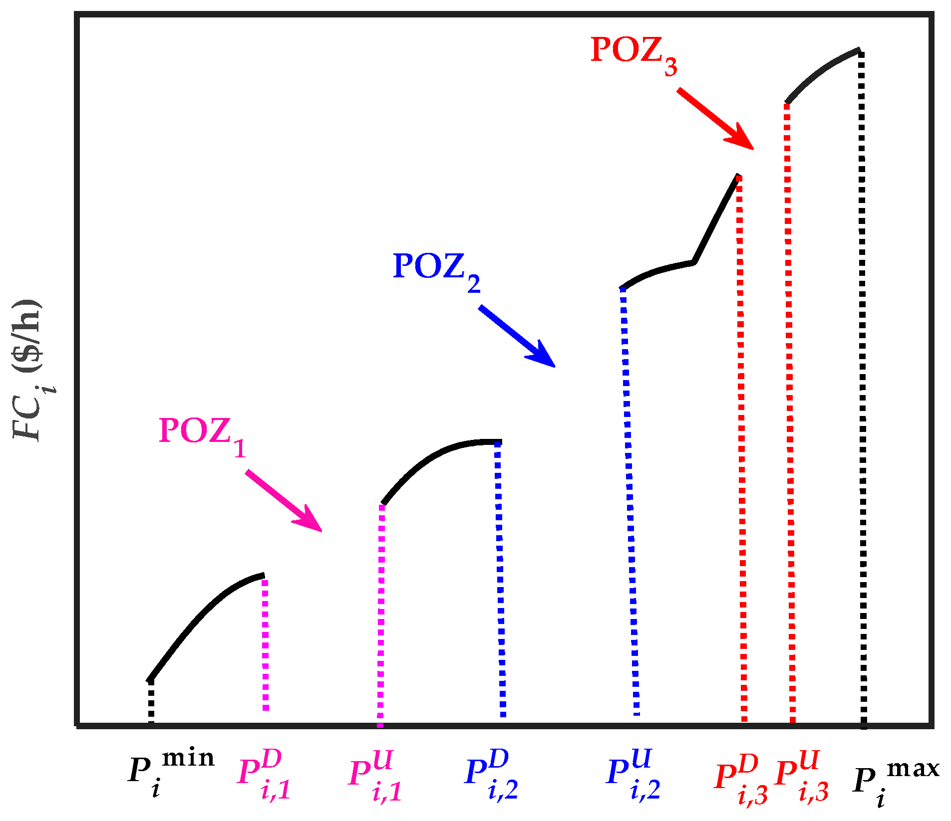
Generally, it is assumed that the power output of a TGU can be continuously adjusted; however, in practice, there are zones or regions of undesirable operations caused by problems related to instability or physical operating limitations at the machine component level. Therefore, power generated must be located outside these zones, which are called POZ constraints. Taking into account these POZs may actually lead to discontinuities in both fuel cost and emissions curves, as shown in Figure 2. For the i-th TGU, the POZ constraints can be described as follows [5].
{ P i min P i P i , 1 D P i , z 1 U P i P i , z D P i , N Z i U P i P i max , z { 2 , 3 , , N Z i }

3. Proposed Optimization Technique

In this section, the main steps of both DE and the proposed ChMODE method are presented. The proposed ChMODE will be applied to solve the nonconvex multiobjective EEDP.

3.1. The Original DE Algorithm

The DE algorithm is inspired by evolutionary strategies and genetic algorithms through selection, mutation, and crossover operators. It has been initially introduced by Storn and Price [35]. In the DE algorithm, real-coded numbers of the decision variables are generally used instead of binary-coded numbers, which allows for reducing its computational complexity. The DE starts with a random initialization of the population of N S  D-dimensional vector solutions [35], as given in Equation (10). Note that the i-th solution in the initial population is in the form of X 0 i = [ x 1 , 0 i x 2 , 0 i x D , 0 i ] .
x k , 0 i = X k min + φ ( X k max X k min ) , i = 1 , , N S and k = 1 , , D
where X k min and X k max are the lower and upper limits of the k-th decision variable. φ is a uniformly distributed random number in the interval ( 0 , 1 ) .
In the DE algorithm, the solutions in the current population Ψ t , at the generation t, are updated by applying mutation, crossover, and selection operators, respectively. The updated solutions constitute the new population Ψ t + 1 corresponding to the next generation ( t + 1 ) . Generally, the DE algorithm principle is as follows.
At each generation t and for each parent vector (target vector) corresponding to the i-th individual in the current population Ψ t , a mutation vector V t i = [ v 1 , t i , v 2 , t i , , v N S , t i ] , which is called the donor vector, is generated by applying the mutation operator. To do this, the donor vector V t i can be obtained according to Equation (11) [36].
V t i = X t r 1 + F ( X t r 2 X t r 3 )
where r 1 , r 2 and r 3 { 1 , 2 , , N S } \ { i } are randomly generated integers for each target vector. F is a scaling factor, which is usually chosen from the interval ( 0.2 , 1 ) and used to control the difference between X t r 2 and X t r 3 .
Once the donor vector is generated, a crossover operation between the donor vector V t i and the target vector X t i is applied to improve the population diversity. One of the most commonly used crossover strategies is the binomial crossover which is applied in this study. Therefore, the offspring solution, which is known as a trial vector and denoted by U t i = [ u 1 , t i , u 2 , t i , , u N S , t i ] , can be obtained as follows [36].
u k , t i = { v k , t i if ( θ k i C r ) or ( k = k r a n d ) x k , t i otherwise
where θ k i ( 0 , 1 ) is a uniform random number generated for each decision variable. C r ( 0 , 1 ) is the crossover probability. k r a n d { 1 , 2 , , N S } is a randomly generated integer.
The main steps of a DE algorithm are described in Figure 3. As given in this figure, after setting its main parameters, the DE algorithm starts by randomly generating NS initial solutions according to Equation (11). Each solution from the initial population is represented by a vector X 0 i = [ x 1 , 0 i x 2 , 0 i x D , 0 i ] . Then, the mutation operator is applied to all solutions X t i of the actual population to generate a new set of vectors V t i , where t is the iteration number. To do this, for every solution X t i , three solutions are randomly chosen from the actual population, and then, a weighted difference in two solutions among these selected solutions is added to the third one, as given by Equation (11). After generating mutation vectors of all parent solutions, each couple of parent solution X t i and its mutation vector V t i undergo a crossover process to generate a new vector solution U t i , as given by Equation (12). Finally, a greedy selection between X t i and U t i vectors is carried out to choose which solution will survive in the next population Ψ t + 1 . This process continues until a predefined maximum number of iterations is reached or a desired value of the fitness function is achieved.

3.2. Proposed ChMODE Algorithm

In various works such as [34,35,36,37], it has been shown that the DE algorithm has demonstrated good performance and strong robustness in handling several nonlinear and multimodal optimization problems. However, DE has the disadvantage of being trapped in local optima; it is time-consuming and has poor search ability when solving complex, highly nonlinear optimization problems [51]. One of the main causes of these issues is linked to random variables involved in the various steps of the DE algorithm. To cope with this, an improved version of DE utilizing chaotic sequences instead of random numbers is presented in this section, which is one of the main contributions of the current work. Indeed, it has proved that a chaotic system encloses important features that can be interesting for the improvement of stochastic optimization algorithms, such as its ergodicity property and dependence on initial conditions [5].
In the proposed chaotic multiobjective DE algorithm (ChMODE), two different chaotic maps are applied in the population initialization, mutation, and crossover phases. These chaotic maps are described below.

3.2.1. Logistic Map

A logistic map, which has been first developed by May [65], is a one-dimensional (1-D) discrete chaotic system. It generates chaotic sequences, which can be mathematically described as follows [61]:
x k + 1 L M = r x k L M ( 1 x k L M ) , k = 1 , 2 , , N L M
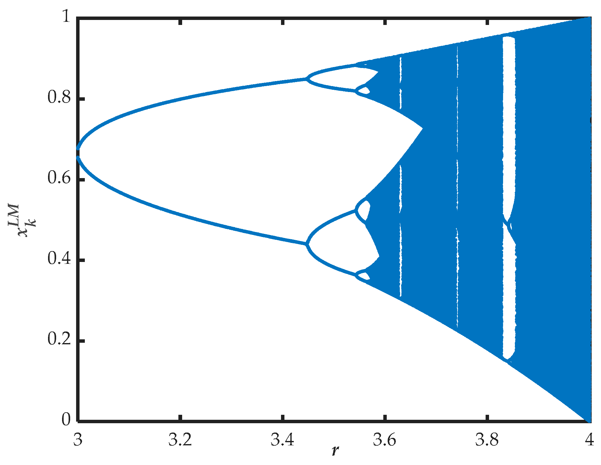
where x k L M is the state variables of the logistic map. Note that x k L M ( 0 , 1 ) for the condition x 0 L M ( 0 , 1 ) . r ( 0 , 1 ) is the control parameter of the logistic map. In order to have a chaotic behavior, r should be in the interval ( 3.569945672 , 4 ) [66]. The bifurcation diagram of the logistic map is presented in Figure 4.
In Equation (15), N L M is the number of chaotic numbers generated by the logistic map. It is to be noted that a logistic map is used in this study to generate pseudonumbers φ and θ k i involved in Equations (11) and (13), respectively. Therefore, N L M is calculated as follows:
N L M = ( G e n max + 1 ) N S × D
where G e n max is the maximum number of generations in the DE algorithm.
Pseudonumbers φ and θ k i are regenerated as below.
Let us consider the following two matrices, which are filled with the logistic map sequences ( x k L M ).
Φ L M = [ x 1 L M x 2 L M x D L M x D + 1 L M x D + 2 L M x 2 D L M x ( N S 1 ) D + 1 L M x ( N S 1 ) D + 2 L M x ( N S ) D L M ]
Θ L M , t = [ x t N S D + 1 L M x t N S D + 2 L M x ( t N S + 1 ) D L M x ( t N S + 1 ) D + 1 L M x ( t N S + 1 ) D + 2 L M x ( t N S + 2 ) D L M x { ( t + 1 ) N S 1 } D + 1 L M x { ( t + 1 ) N S 1 } D + 2 L M x ( t + 1 ) N S D L M ] , t = 1 , 2 , , G e n max
Note that Pseudonumbers φ and θ k i can be extracted from matrices Φ L M and Θ L M , t , respectively.
By applying the logistic map for the population initialization and crossover process, Equations (10) and (12) become as given in Equations (17) and (18), respectively.
x k , 0 i = X k min + Φ L M ( i , k ) ( X k max X k min ) , i = 1 , , N S and k = 1 , , D
u k , t i = { v k , t i   ,     if ( Θ L M , t ( i , k ) C r ) or ( k = k r a n d ) x k , t i   ,     otherwise  

3.2.2. Lorenz Attractor

The Lorenz attractor was introduced by Edward Lorenz [67] for modeling the phenomenon of thermal convection in fluids. Mathematically, the Lorenz attractor is described by a three-dimensional system of ordinary differential equations, as follows [68].
{ d x L A d t = γ ( y L A x L A ) d y L A d t = x L A ( ρ z L A ) y L A d z L A d t = x L A y L A δ z L A
where x L A , y L A , and z L A are the state vectors of the Lorenz attractor. Note that these vectors are of the same size. γ , ρ , and δ are the Lorenz attractor parameters. Typical values of these constants are as follows [68].
γ = 10 , ρ = 28 and δ = 8 / 3 .
Because Lorenz attractor is a three-dimensional system, it is adopted in the mutation process to regenerate the three random numbers involved in Equation (11) where the state vectors x L A , y L A , and z L A are used in that equation instead of r 1 , r 2 and r 3 , respectively. Therefore, the size N L A of each state vector can be calculated as given by Equation (20).
N L A = G e n max N S
For presentation convenience, let us consider
x L A = ( x 1 L A , x 2 L A , , x N L A L A )
y L A = ( y 1 L A , y 2 L A , , y N L A L A )
z L A = ( z 1 L A , x 2 L A , , z N L A L A )
In addition, let us consider
R 1 = [ x 1 L A x 2 L A x N S L A x N S + 1 L A x N S + 2 L A x 2 N S L A x ( G e n max 1 ) N S + 1 L A x ( G e n max 1 ) N S + 2 L A x G e n max N S L A ]
R 2 = [ y 1 L A y 2 L A y N S L A y N S + 1 L A y N S + 2 L A y 2 N S L A y ( G e n max 1 ) N S + 1 L A y ( G e n max 1 ) N S + 2 L A y ( G e n max ) N S L A ]
R 3 = [ z 1 L A z 2 L A z N S L A z N S + 1 L A z N S + 2 L A z 2 N S L A z ( G e n max 1 ) N S + 1 L A z ( G e n max 1 ) N S + 2 L A z ( G e n max ) N S L A ]
Therefore, Equation (11) becomes as follows.
V t i = X t R 1 ( t , i ) + F ( X t R 2 ( t , i ) X t R 3 ( t , i ) )

3.2.3. NonDomination Sorting

The EEDP is a MOP, which leads to a set of solutions, commonly called Pareto solutions or nondominated solutions, instead of a single optimal solution. A large number of recent research works have combined both the economic and the emission functions in a single-objective function using the weighted-based sum method and price penalty factor (PPF) [5,17,32]. However, weighted-based sum methods cannot provide the PF in a single run. In order to generate the PF of nondominated solutions, the weighted-based sum method must be run for various values of the weighting factor. Moreover, it can fail to achieve an accurate and true PF for nonconvex problems. Therefore, a multiobjective optimization able to simultaneously minimize fuel cost and emissions is recommended. Within this context, the proposed ChMODE method is adopted for the bi-objective EEDP by adding the nondomination principle and crowding distance calculation into the DE algorithm.
In order to find an accurate optimal PF, all solutions of the parent population Ψ t and the offspring population Γ t are prioritized according to the nondomination sorting principle [52]. To do this, at every iteration t, the parent and offspring populations are grouped in a common population R t , as follows.
R t = Ψ t Γ t
After that, population R t is subdivided into different fronts F i , based on their nondomination levels. F 1 is the set of all nondominated solutions extracted from R t , and F i is the set of nondominated solutions extracted from R t \ ( k = 1 i 1 F k ) for i > 1 . Therefore, population R t can be described as follows.
R t = k = 1 s F k
where s is the number of fronts.
Solutions in each front F i are ranked according to their crowding distances in ascending order. The next population, Ψ t + 1 , will be filled by NS solutions selected from R t according to the level of fronts to which they belong and their ranks. Thus, if the size of F 1 is greater than or equal to NS, then only the NS least crowded solutions are selected to form Ψ t + 1 . If not, then all solutions of F 1 are directly added into Ψ t + 1 . The remaining solutions of Ψ t + 1 are selected from the next front, F 2 , according to their crowded distances. If the size of Ψ t + 1 is still less than NS, then this process is applied for the next fronts until the size of Ψ t + 1 is equal to NS. The main steps of the generation of the new population Ψ t + 1 based on the domination-sorting process and crowding distance calculation are summarized in Algorithm 2.
Algorithm 2: Pseudocode of the generation of a new population.
   1. Inputs: Parent population Ψ t
     Offspring population Γ t
    2. Outputs: New population Ψ t + 1
    3. Combine Ψ t and Γ t
         R t = Ψ t Γ t
    4. Apply nondomination sorting of R t
        4.1. i = 1
        4.2. F i = P a r e t o _ d o m i n a n c e ( R t )
        4.3. Ψ t + 1 = F i
        4.4. While ( | Ψ t + 1 | < | Ψ t | ) do
          4.4.1. i = i + 1
          4.4.2. F i = P a r e t o _ d o m i n a n c e ( R t \ Ψ t + 1 )
          4.4.3. Ψ t + 1 = Ψ t + 1 F i
        4.5. End
    5. If ( | Ψ t + 1 | > | Ψ t | ) do
        5.1. Calculate crowding distance of all members of F i
        5.2. Sort F i according to the crowding distances of its members in ascending order
        5.3. Ψ t + 1 = Ψ t + 1 \ F i
        5.4. While ( | Ψ t + 1 | < | Ψ t | ) do
             Ψ t + 1 = Ψ t + 1 { F j i } ; F j i is the j-th member of the sorted set F i
        5.5. End While
    6. End If
In the conventional DE algorithm, the initial population, crossover, and mutation stage are based on random numbers, which may slow down the convergence speed of the algorithm and may lead to a local optimum. To overcome these drawbacks, these random numbers are replaced by chaotic sequences in the suggested ChMODE. Hence, ChMODE starts by generating the logistic map sequences { x k L M } and Lorenz attractor sequences which are { x k L A } , { y k L A } , and { z k L A } . These sequences are used to form matrices Φ L M , Θ L M , R 1 , R 2 , and R 3 as given by Equations (15), (16), and (24)–(26), respectively. The next step in the ChMODE is the creation of the initial population according to Equation (17). At each iteration t, a mutation vector is generated for each solution (donor vector) of the current population Ψ t , according to Equation (27). Once all mutation vectors are generated, a crossover process between each mutation vector and its donor vector is applied, according to Equation (28). The obtained solutions (trial vectors) will constitute the offspring population ( Γ t ). In order to obtain the new population, the parent population Ψ t and offspring population Γ t are combined into one population. Then, the nondomination sorting process and crowding distance calculation are applied as presented in Algorithm 2 to generate the PF and the new population Ψ t + 1 . To summarize, the main steps of the ChMODE technique proposed for solving the EEDP can be illustrated in Algorithm 3.
Algorithm 3: Pseudocode of the ChMODE for solving the EEDP.
   1. Inputs: Power network data
     DE parameters
     Chaotic maps parameters
    2. Outputs: Optimal power output of thermal units
     Optimal operating cost
     Optimal emissions
    3. Generation of chaotic sequences
       3.1. Generate logistic map sequences { x k L M }
       3.2. Generate Lorenz attractor sequences { x k L A } , { y k L A } , and { z k L A }
       3.3. Construct matrices Φ L M , Θ L M , R 1 , R 2 and, R 3
    4. Population initialization
       4.1. For i = 1 to NS do
         4.1.1. For k = 1 to D do
             x k , 0 i = X k min + Φ L M ( i , k ) ( X k max X k min )
         4.1.2. End For
       4.2. End For
    5. Application of mutation, crossover, and selection operators
        t = 0
       5.1. While ( t < G e n max ) do
         5.1.1. t = t + 1
         5.1.2. Γ t =
         5.1.3. For i = 1 to N S do
            V t i = X t R 1 ( t , i ) + F ( X t R 2 ( t , i ) X t R 3 ( t , i ) )
           5.1.3.1. For k = 1 to D do
               Generate random number k r a n d
               5.1.2.1.1. If ( Θ L M , t ( i , k ) C r ) or ( k = k r a n d ) do
                      u k , t i = v k , t i
               5.1.2.1.2. Else
                      u k , t i = x k , t i
               5.1.2.1.3. End If
           5.1.3.2. End For
           Evaluate f ( X t i ) and f ( U t i ) according to Algorithm 1
            Γ t = Γ t { U t i }
         5.1.4. End For
         5.1.5. Generation of the new population Ψ t + 1 according to Algorithm 2
       5.2. End While
    6. Print the optimal generation of thermal units
The proposed ChMODE algorithm is a combination of the DE method and chaotic maps. Therefore, the computational complexity of this algorithm depends on the generation of chaotic sequences and the DE mechanism. In the DE, the computing time complexity for the initialization of the population is O ( N S ) , where N S is the population size. Fitness calculation also needs O ( N S ) . In addition, generating a mutation vector needs computing time complexity of O ( N S 2 ) in the worst case, whilst fitness calculation and crossover operation need O ( N S ) and O ( 2 N S ) , respectively. In the ChMODE algorithm, the one-dimensional logistic map and the three-dimensional Lorenz attractor are used. Thus, it needs a computing time complexity of O ( 4 N S ) for generating the chaotic sequences. Accordingly, an overall time complexity of ChMODE is O ( N S 2 ) in the worst case.

4. Case Studies and Simulation Results

In this section, the feasibility and effectiveness of the proposed optimization technique ChMODE for solving the dispatch problem are validated under three case studies with various complexity levels. These systems have been widely employed as benchmarks for testing and validating various strategies and techniques suggested in the power system field. The results for the ChMODE are compared with those obtained with other optimization techniques recently published. Meanwhile, to demonstrate the impact of the proposed chaotic maps in speeding up the convergence of the proposed algorithm, the convergence characteristics of the ChMODE for minimizing cost and emission functions are compared with the classical DE, ABC, and invasive weed optimization (IWO) algorithms. These techniques are implemented in Matlab software and run on a CPU Intel Core i7 with 8 GB of random access memory (RAM). For a fair comparison, these algorithms are executed with the same population size and maximum number of iterations which are equal to 300 and 200, respectively. All optimal results are obtained after 30 runs of the ChMODE method. The parameters’ values and operators of the compared algorithms are tabulated in Table 2.
In order to further show the accuracy of the proposed algorithm, a criterion for measuring the violation of the power balance constraint described by Equation (6) is used. As a matter of fact, inequality constraints can be easily fulfilled when using metaheuristic techniques; however, the satisfaction of equality constraints presents some difficulties. For that, a violation criterion of constraints is employed by different swarm intelligence-based techniques. For dispatch problems, this criterion is expressed by Equation (30), and it can be employed to verify if the total generation can meet the total load or not.
Δ P = | i = 1 N G P i ( P l d + P t l ) |
In order to have Δ P = 0 , the power outputs of all TGUs except the slack generator are optimally determined by the ChMODE. Then, transmission losses and power output of the slack generator are calculated according to Algorithm 1.

4.1. Case 1: Six-Unit System

In this case, the six-unit system composed of six generating units with quadratic cost and emission functions is used to evaluate the effectiveness of the proposed ChMODE algorithm. All system data, including fuel cost coefficients, emission coefficients, and generation limits, are stated in [69]. The units’ data of the six-unit system are tabulated in Table A1. The system B-loss matrix is as follows.
B = [ 1.40 0.17 0.15 0.19 0.26 0.22 0.17 0.60 0.13 0.16 0.15 0.20 0.15 0.13 0.65 0.17 0.24 0.19 0.19 0.16 0.17 0.71 0.30 0.25 0.16 0.15 0.24 0.30 0.69 0.32 0.22 0.20 0.19 0.25 0.32 0.85 ] 10 4
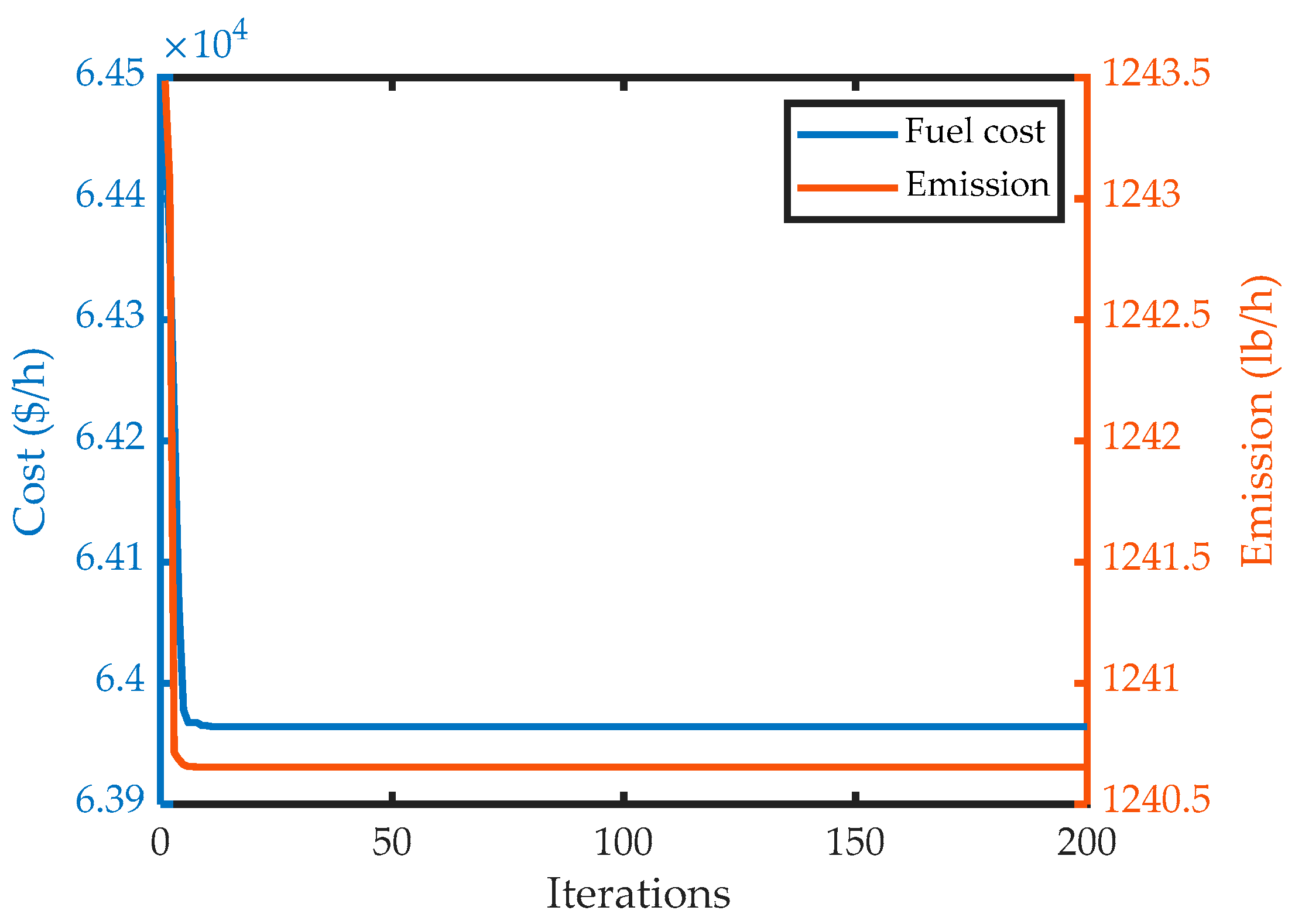
The EEDP is solved by using the proposed ChMODE for a total system load equal to 1200 MW. Since EEDP is a multiobjective problem, the performance of the proposed method in finding the extreme points of the PF, which correspond to the economic dispatch problem (EcDP) and emission dispatch problem (EmDP), must be investigated. Figure 5 displays the convergence behaviors of the ChMOED for minimizing cost and emission functions. It is to be noted that the ChMODE converges speedily to the optimal solutions, whether for the best fuel cost or best emission. By applying the ChMODE, minimum cost and minimum emission are obtained after 12 and 10 iterations, respectively.
Optimal units’ outputs of the studied system, in MW, for minimum fuel cost and minimum emission obtained using ChMODE and other techniques, such as QOTLBO [70], EMOCA [71], DE [69], BSA [72], and NSGA-III [29] are tabulated in Table 3 and Table 4, respectively. Generally speaking, Table 3 shows that the proposed ChMODE method has the best results for the economic dispatch case, where the minimum fuel cost is 63,963.96 $/h. Compared with BSA, which corresponds to the second-best result, ChMODE saves 13.96 $/h fuel cost. However, it can be clearly seen from Table 4 that all methods achieve almost identical results for emission minimization. By applying ChMODE, the minimum emission value is 1240.6 lb/h. Unlike the aforementioned comparative techniques, the power balance constraint is strictly fulfilled where Δ P = 0 .
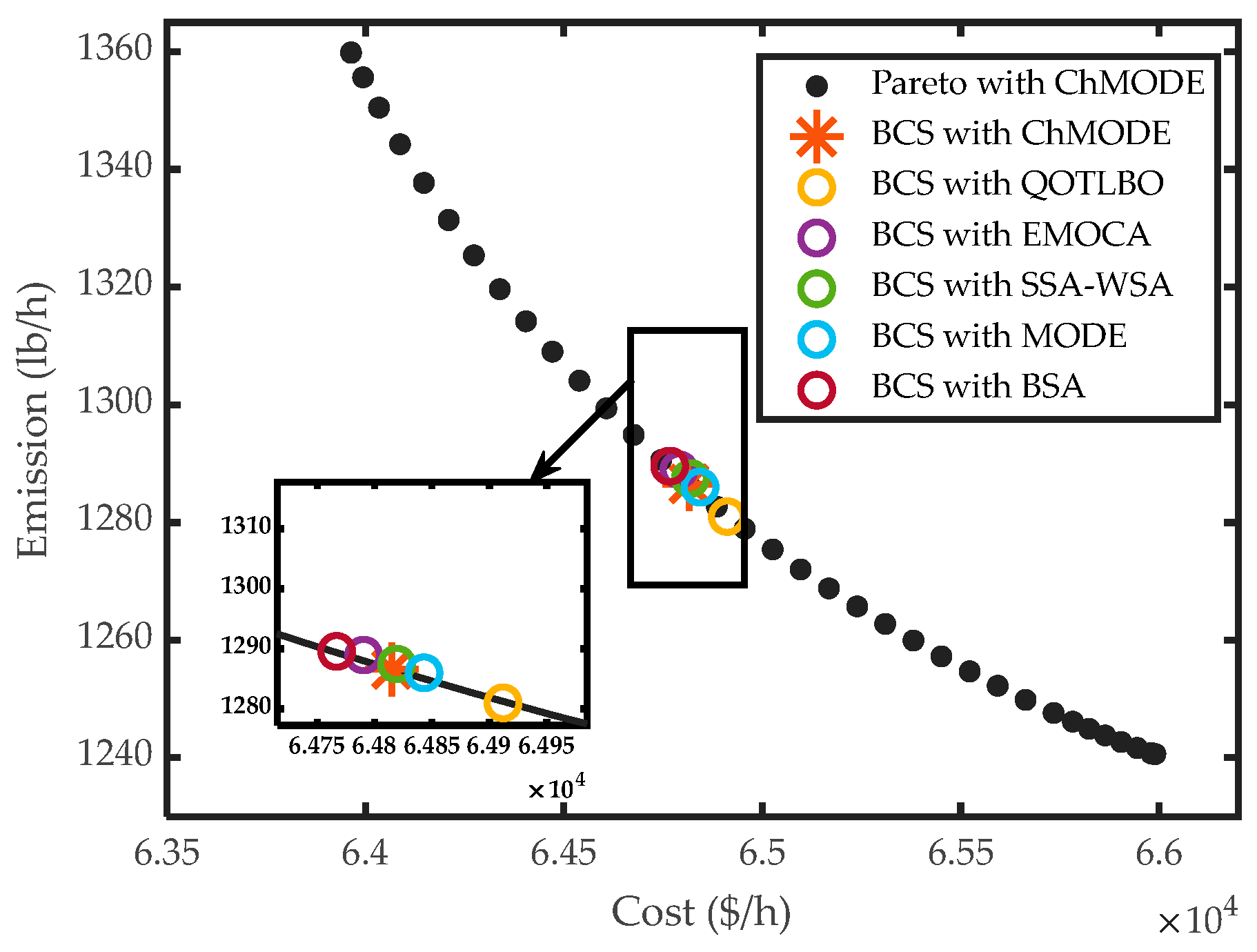
The trade-off curve furnished by ChMODE is shown in Figure 6. This figure clearly shows that the solutions found are well distributed over the entire trade-off surface. The two extreme points of this curve correspond to the optimal solutions of the EcDP and EmDP. Note that the optimal solution corresponding to the minimum fuel cost (63,963.96 $/h) corresponds to the highest value of emission (1359.87 lb/h). In the meantime, the optimal solution for minimum emission (1240.6 lb/h) corresponds to the worst value of fuel cost (65,990.4 $/h). In order to select the best compromise solution (BCS) from the PF for decision-making, a fuzzy-based strategy presented by [66] is used in this study. As shown in Figure 6, the BCS for the studied 6-unit system corresponds to a fuel cost equal to 64,815.143 $/h and an emission of around 1286.563 lb/h. For comparison purposes, BCSs obtained by other methods, including QOTLBO [70], EMOCA [71], SSA-WSA [71], MODE [69], and BSA [72], are illustrated in Figure 6. From this figure, it can be seen that BCSs resulting from EMOCA, SSA-WSA, and MODE are outside the PF. Meanwhile, the ones of QOTLBO and BSA are located on the trade-off curve. The BCS generated by BSA is near the solution of ChMODE.
The optimal generator outputs corresponding to the compromise solutions obtained by ChMODE and the aforementioned comparative methods are tabulated in Table 5. From this table, it is obvious that these solutions are nondominated solutions with respect to each other.

4.2. Case 2: Ten-Unit System without POZs

In this section, a larger system known as the IEEE 30-bus 10-unit system is considered to further test the robustness and performance of the proposed ChMODE for handling the EEDP. In this case study, VPLEs are added to the ordinary quadratic fuel cost function. However, POZ constraints are neglected. Coefficients of the fuel cost and emission functions, as well as generator limits, are adopted from [69]. The units’ data of the ten-unit system are tabulated in Table A2. The system load is assumed to be equal to 2000 MW, and the transmission losses are considered in the power balance equation. The system B-loss matrix is as follows.
B = [ 0.49 0.14 0.15 0.15 0.16 0.17 0.17 0.18 0.19 0.20 0.14 0.45 0.16 0.16 0.17 0.15 0.15 0.16 0.18 0.18 0.15 0.16 0.39 0.10 0.12 0.12 0.14 0.14 0.16 0.16 0.15 0.16 0.10 0.40 0.14 0.10 0.11 0.12 0.14 0.15 0.16 0.17 0.12 0.14 0.35 0.11 0.13 0.13 0.15 0.16 0.17 0.15 0.12 0.10 0.11 0.36 0.12 0.12 0.14 0.15 0.17 0.15 0.14 0.11 0.13 0.12 0.38 0.16 0.16 0.18 0.18 0.16 0.14 0.12 0.13 0.12 0.16 0.40 0.15 0.16 0.19 0.18 0.16 0.14 0.15 0.14 0.16 0.15 0.42 0.19 0.20 0.18 0.16 0.15 0.16 0.15 0.18 0.16 0.19 0.44 ] 10 4
To evaluate the ChMODE effectiveness, various algorithms, including DE [69], KSO [73], QOTLBO [70], BSA [72], OWP-based OMF [30], MOCDOA [31], and NSGA-III [29] are employed for comparison.
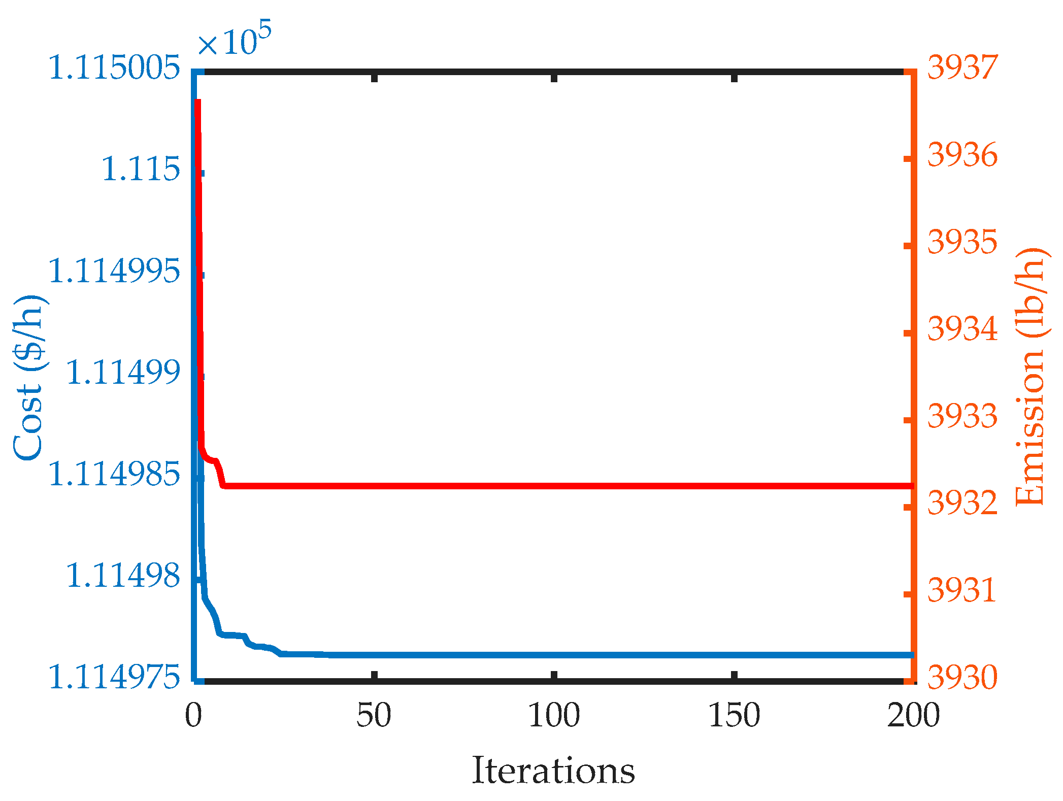
The convergence characteristics of the ChMODE for fuel cost minimization (EcDP) and emission minimization (EmDP) are illustrated in Figure 7. From this figure, it can be noticed that the proposed method swiftly reaches the optimal solutions for both objectives. The best minimum cost and best minimum emission are 111,497.6308 $/h and 3932.2433 lb/h, respectively. Table 6 and Table 7 give the optimal outputs in MW of units P 1 to P 10 for the EcDP and EmDP obtained by ChMODE and the aforementioned comparative methods, respectively. These tables prove that ChMODE provides better results and clearly outperforms many techniques. Moreover, the best results of some techniques are those provided by the suggested algorithm at the initial iteration. This is due to the use of chaotic maps instead of random numbers in the initialization phase of ChMODE. In terms of the equality constraint violation, the ChMODE algorithm has the best results where this constraint is strictly constraint ( Δ P = 0 ) for both EcDP and EmDP.
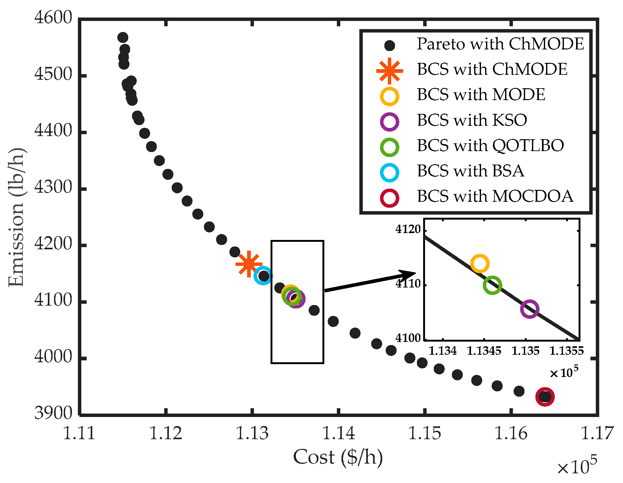
Since this case is also a multiobjective problem, nondominated optimal solutions should be attained for the EEDP. To do this, the fuel cost and emission functions are simultaneously minimized by the proposed method. In this way, a set of nondominated solutions representing the PF can be generated after the convergence of the ChMODE algorithm. Values of cost and emission of some nondominated solutions are tabulated in Table 8. From this table, it is obvious that the more the total emissions increase, the more the fuel cost decreases and vice versa.
Figure 8 depicts the PF attained by the ChMODE algorithm. As is shown in this figure, nondominated solutions are well distributed over the PF, and fuel cost and emission functions are conflicting objectives. Furthermore, to assess the competitive efficacy of the proposed technique, BCSs obtained by ChMOED and other techniques reported in the literature are presented in Figure 8. From Figure 8, it can be clearly seen that BCSs obtained by MODE and QOTLBO algorithms are outside the trade-off curve. Moreover, BCSs obtained by MOCDOA coincides with the best emission solution, which implies that the importance given to the economic aspect is neglected. However, BCSs provided by the BSA technique is close to that of ChMODE. Optimal generations corresponding to the BCSs of all system units obtained by various techniques are illustrated in Table 9.
In order to further evaluate the robustness of the proposed ChMODE algorithm for handling complex optimization problems, such as EEDP, statistical results comprising best, mean, worst, and standard deviation (Std) values of production cost and emissions are tabulated in Table 10. Statistical results are determined over 30 runs of the ChMODE, SAIWPSO [74], OWP-OMF [30], and GQPSO [73] techniques. From these results, it can be clearly concluded that the ChMODE algorithm outperforms the other random-based algorithms in terms of stability and accuracy. In fact, the proposed ChMODE technique has the lowest mean and standard deviation values for both fuel cost and emission functions.

4.3. Case 3: Test System 2 with POZ Constraints

In this case, POZs of the 1st, 2nd, 9th, and 10th TGUs of the ten-unit system are considered together with VPLEs and total transmission losses. Thus, the complexity level of the EEDP is increased by introducing discontinuities into the fuel cost and emission functions. The system load is assumed to be equal to 2000 MW, and POZs of the ten-unit system TGUs are illustrated in Table 11.
Knowing that this case has not been studied in previous research works, the convergence characteristics and performance of the ChMODE are compared with those of DE, ABC, and IWO techniques which are implemented using Matlab software with the same population size and maximum number of generations as ChMODE algorithm. The convergence behaviors of the ChMODE as well as the comparative algorithms for fuel cost minimization and emission minimization, are shown in Figure 9. At first glance, it can be clearly observed that ChMODE exhibits fast convergence into the optimal solutions compared to the other algorithms. Moreover, the proposed technique starts from the lowest values for both cost and emission functions. This proves that ChMODE is improved from the aspects of initial population and convergence rate. Optimal output powers of units obtained after convergence of the ChMODE, DE, ABC, and IWO for EcDP and EmDP are tabulated in Table 12. According to this table, it is obvious that ChMODE provides the best results. Moreover, it can be clearly seen that the minimum emission that corresponds to Case 3 is increased. Indeed, the emission is augmented from 3932.2433 lb/h (in Case 2) to 3965.61212 lb/h (in Case 3). This is due to the inclusion of POZs in the EEDP constraints. In fact, adding constraints to an optimization problem may lead to a limitation in the search space and therefore restrict the values that objective functions can take.
Table 13 shows the statistical results for both EcDP and EmDP obtained by ChMODE, DE, ABC, and IWO algorithms for Case 3 over 30 rums. From this table, it can be noted that ChMODE yields significantly better results than the compared optimization algorithms from the point of view of robustness and results accuracy.
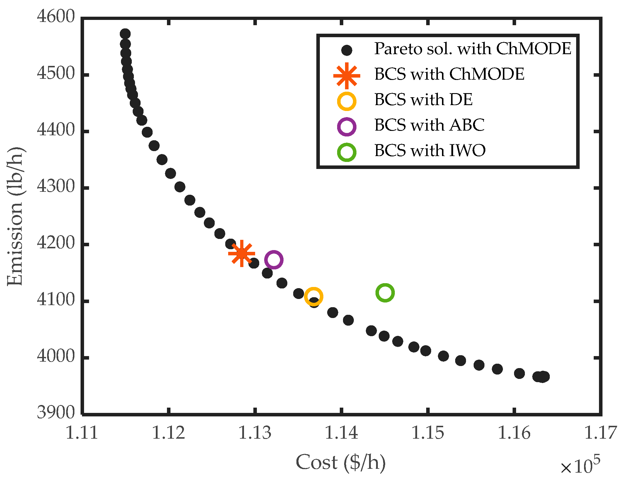
The performance of the suggested ChMODE algorithm is also tested when cost and emission functions are simultaneously minimized under Case 3. Figure 10 illustrates the PF furnished after the convergence of the ChMODE. This figure also illustrates the BCSs of ChMODE together with those obtained by the compared algorithms. It can be noted from this figure that trade-off points are well distributed in the objective space. It can also be seen that the shape of the PF found by using the proposed method is similar to the shapes of all EEDP Pareto fronts obtained in other references [3,11,67,69]. This PF shape is due to the fact that cost and emission functions are conflicting objectives. This implies that by minimizing the fuel cost, the emission increases and vice versa.
Figure 10 also shows that the BCSs for the ABC and IWO algorithms are placed above the PF. Furthermore, it can be clearly seen that the BCS of IWO is dominated by solutions from the PF. Optimal generations that correspond to these BCSs are tabulated in Table 14, which clearly shows that all power outputs do not belong to the POZs.

4.4. Robustness Analysis

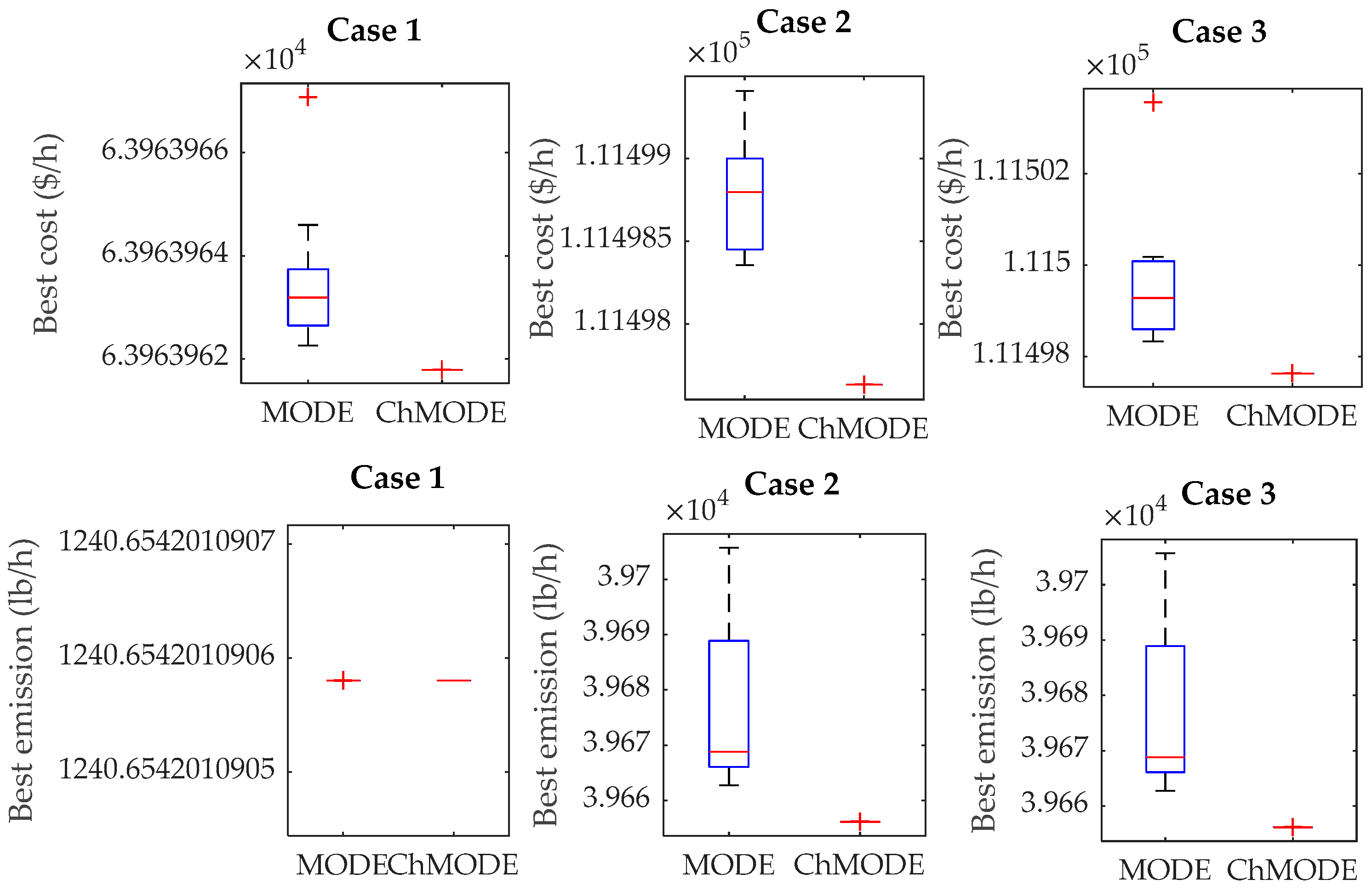
In order to further evaluate the robustness of the proposed ChMODE for solving the nonconvex EEDP, seven well-known multiobjective optimization methods, including MOCDOA [31], MODE [69], MOPSO [31], NSGA-II [31], MOSSA [75], PESA-II [31], and NSPSO [76], are adopted and compared with ChMODE. In this subsection, the performance of the ChMODE algorithm, when looking for the extreme points of the PF, is compared with MODE [50] for Cases 1, 2, and 3. Note that both algorithms are implemented with the same population size and maximum number of iterations. Figure 11 shows the boxplots for the best cost and best emission obtained after 30 runs of ChMODE and MODE algorithms. From this figure, it is clear that the distribution of best solutions obtained by ChMODE is more centralized than MODE. Moreover, unlike MODE, there are no outliers for the ChMODE algorithm. This can prove the high stability of the proposed algorithm compared to the MODE algorithm.
To evaluate the distribution of the obtained nondominated solutions and their proximity to the actual Pareto set, three performance indicators comprising inverted generational distance (IGD), hyper-volume (HV), and spacing metric (SM) [65] are used and measured. Here, Case 2 is adopted due to the availability of the Pareto solutions set in various studies, such as reference [60], which can be considered as an approximation of the true optimal PF.
The IGD indicator is used to measure the capability of an optimization technique to converge to the PF at the nearest distance to the optimal PF. A lower value of this indicator signifies better performance. The IGD can be expressed as follows [65].
I G D = 1 N P F i = 1 N P F d i 2
where N P F is the number of solutions in the optimal PF. d i is the Euclidean distance between the i-th solution of the obtained PF and the optimal PF.
The second indicator, which is HV, is widely chosen to evaluate the convergence and distribution of a set of solutions. Larger values of HV signify a better set of solutions. This indicator can be expressed as follows [65].
H V ( A , r ) = V ( a A { b | a _ b _ r } )
where V ( ) is the Lebesgue measure. A m is a set point, and r m is a reference point. a _ b means that solution a dominates solution b.
In order to evaluate the distribution of the nondominated solutions through the optimal PF, the spacing metric (SM) is used. This metric can be calculated by Equation (35) [77].
S M = 1 N P F 1 i = 1 N P F ( d i d ¯ ) 2
where d ¯ is the average of all d i .
A small value of SM signifies that the obtained solutions are evenly distributed in the PF.
Given the importance of the compromise solution for power system decision-makers, the performance of the proposed method from the point of view of compromise solution quality is checked in this study by calculating the average satisfactory degree (ASD) of the decision-maker. Indeed, one of the main challenges in EEDPs is the selection of the best compromise solution among the PF rather than deploying all Pareto solutions, which can facilitate the mission for the decision maker to perform the appropriate decision. The ASD value is calculated according to the extreme points of the PF shown in Table 6 and Table 7.
Generally, the decision makers’ opinion is not precise for real problems such as EEDP; thus, a fuzzy-based approach [62] is adopted to evaluate the decision maker’s satisfaction with the optimal solution. The satisfactory degree of a nondominated solution X i for the k-th objective function F k can be expressed by the following membership function [62].
μ k i = { 1 , F i ( X i ) F k min F k max F i ( X i ) F k max F k min , F k min < F i ( X i ) < F k max 0 , F i ( X i ) F k max
where F k min and F k max are minimum and maximum values of F k , respectively.
The normalized membership function corresponding to the nondominated solution X i is given by
μ i = k = 1 m μ k i i = 1 N P F k = 1 m μ k i
where m is the number of objective functions.
Let us consider a compromise solution X c s . Thus, its ASD can be calculated using the following expression [62].
A S D c s = 1 m k = 1 m μ k c s
A comparison of the results for the aforementioned indicators, obtained by the proposed ChMODE and other reported methods, is shown in Table 15. Note that NR in this table denotes that the indicator is not reported. Indeed, very few research papers have used these indicators to test the performances of multiobjective techniques when applied to EEDP. From Table 15, it can be clearly seen that ChMODE provides the highest ASD among the other methods, which implies that ChMODE provides the best compromise solutions. Moreover, by investigating IGD and HV indicators, it can be seen that ChMODE is more efficient than the other algorithms from the viewpoint of diversity and convergence. In fact, the ChMODE has the lowest value of the IGD indicator, which implies that it generates the nearest nondominated solutions to the true optimal PF. The ChMODE algorithm provides the highest value for HV, which signifies that optimal solutions of its PF are more distributed compared to MODE and NSPSO algorithms. The superiority of the proposed method in terms of the diversity of nondominated solutions can also be proved by investigating the SM indicator. Indeed, ChMODE has the lowest SM value compared to the classical MODE. Hence, integrating chaotic maps in stochastic optimization methods can enhance their search ability and diversity of the optimal solutions.

4.5. Results Discussion and Limitations

Generally, the power balance constraint, an equality constraint, has to be enforced in power dispatch problems. However, in various research works, this constraint has been converted into an inequality constraint using violation criteria. This may lead to an inexactitude of the optimal solutions. In this study, the power balance constraint is considered in such a way that the difference between the total generation and the demand power plus total system losses is zero. This condition is considered for all studied cases.
According to the statistical results obtained in this study, it can be concluded that chaotic sequences helped the ChMODE algorithm to enhance its convergence rate, increase the diversity of the obtained solutions and improve the extreme solutions’ quality as well as the compromise solution. Moreover, using chaotic sequences instead of random numbers in the original DE improved its stability. Indeed, the ChMODE achieved the lowest standard deviation compared to the other algorithms, which were 9.39 × 10⁻¹² and 2.96 × 10⁻⁹ for Cases 2 and 3, respectively.
In order to test the robustness of the proposed multiobjective optimization method in solving the nonconvex multiobjective EEDP, the PF and BCS generated by ChMODE are compared with those of various well-known multiobjective optimization methods. In this comparison, various performance indicators, such as ASD, IGD, and HV, are used.
In this study, various comparison methods, including single-objective and multiobjective optimization techniques, are used to show the high performance of the ChMODE for handling the EEDP. These methods are adopted because they have been applied for the same purpose and the same test systems. Furthermore, they have shown good performance and superiority when they have been compared with other powerful techniques. The research studies where these techniques have been published are used for collecting the required data and information.
Although ChMODE performs well in solving the EEDP, there is still a potential effort to enhance this approach in some respects. In fact, various state-of-the-art multiobjective optimization algorithms based on DE have been proposed and tested on real-world optimization problems. Thus, combining the advantages of chaos theory and one of these methods, such as MOEA/D-DE [40], can result in a more accurate optimal PF. Given that true optimal Pareto fronts of EEDPs are not available in the literature, the performance of any suggested multiobjective optimization technique must be first evaluated by using mathematical benchmark models. Descriptions and true optimal Pareto fronts of these models are available in various research works, such as reference [52].

5. Conclusions

In this study, a new chaotic-based multiobjective DE is developed and applied to solve the EEDP. In the suggested ChMODE algorithm, the nondomination principle, as well as crowding distance calculation, is added to provide an accurate PF. In order to make the problem more practical, system power losses, VPLE and POZ constraints are considered in the problem formulation. Unfortunately, adding these constraints to the original EEDP makes it more complex and with discontinuities. Subsequently, classical stochastic optimization methods may fail to provide the global optimal solution due to their random search process. In this respect, all random numbers involved in the original DE phases are substituted by chaotic sequences.
In order to test the robustness and applicability of the proposed ChMODE method, the six-unit and ten-unit systems under various complexities are investigated. By employing the ChMODE algorithm, the total cost is reduced from its maximum to its minimum values by 3.1%, 4.2%, and 4.2% for Cases 1, 2, and 3, respectively. Similarly, the emissions are reduced from their maximum to their minimum values by 8.8%, 14%, and 13.3% for Cases 1, 2, and 3, respectively. Moreover, the power balance constraint is verified for all cases. To further evaluate the performance of the proposed multiobjective ChMODE algorithm, obtained results are compared with other optimization techniques already presented and applied for the same purpose. By investigating the experimental results based on different indicators, including ASD, IGD, SM, and HV, it is shown that ChMODE has the best performance in solving the EEDP with multiple local optima. Accordingly, one of the significant inferences to be deducted from this study is that ChMODE can be an efficient method for handling the nonlinear and nonconvex EEDP regardless of the number of constraints and the number of TGUs. In addition, results obtained by ChMODE, as compared with other single-objective and multiobjective methods, showed the superiority of the suggested method in terms of algorithm stability, distribution of the nondominated solutions, extreme points of the PF, and optimal compromise solution quality. Hence, the proposed method can help the decision maker to perform the appropriate decision for any power network load.
Thanks to the best results furnished by the ChMODE algorithm due to the chaotic proprieties, using the proposed method for solving the dynamic EEDP and other multiobjective problems in the field of power systems remains a future work.

Author Contributions

Conceptualization, A.A. and T.G.; methodology, A.A. and T.G.; software, A.A., T.G. and S.A.; validation, T.G.; formal analysis, A.A. and S.A.; investigation, T.G.; resources, A.A. and T.G.; writing—original draft preparation, A.A. and T.G.; visualization, S.A.; supervision, T.G.; project administration, A.A.; funding acquisition, A.A. All authors have read and agreed to the published version of the manuscript.

Funding

This research has been funded by the Scientific Research Deanship at the University of Ha’il–Saudi Arabia, through project number BA-2128.

Data Availability Statement

Not applicable.

Conflicts of Interest

The authors declare no conflict of interest.

Nomenclature

TCTotal fuel cost in $/h
TETotal emissions in lb/h
T C max Total fuel cost corresponding to the maximum generation
T E max Total emissions corresponding to the maximum generation
F C i Fuel cost of the i-th unit in $/h
E M i Emissions of the i-th unit in lb/h
P i Generation of the i-th unit in MW
N G Number of TGUs
P i min   and   P i max Lower and upper limits of generation in MW for the i-th unit, respectively
P l d Total load demand in MW
P t l Total real power losses in MW
B i j The ij-th element of the matrix of the loss coefficients
P i , z D   and   P i , z U Down and up limits of the z-th POZ of the i-th TGU
N Z i Number of POZs of the i-th TGU
POZiThe i-th POZ of a TGU
NSPopulation size
DNumber of decision variables
X t i The i-th solution at the t-th iteration
x k , 0 i k-th decision variable of the i-th solution in the initial population
N L M Length of the chaotic sequences generated by the logistic map
N L A Length of the chaotic sequences generated by the Lorenz attractor
Ψ t Parent population at the t-th iteration
Γ t Offspring population at the t-th iteration
{ x k L M } Logistic map sequences
{ x k L A } ,   { y k L A }   and   { z k L A } Lorenz attractor sequences

Appendix A

Table A1. Units’ data for the six-unit system.
Unitsaibici α i β i γ i P i max P i min
1756.8038.53900.1524713.85930.327670.0041912510
2451.3346.15910.1058713.85930.327670.0041915010
31050.0040.39650.0280340.2669−0.545510.0068322535
41243.5338.30550.0354640.2669−0.545510.0068321035
51658.5736.32780.0211142.8955−0.511160.00461325130
61356.6638.27040.0179942.8955−0.511160.00461325125
Table A2. Units’ data for the ten-unit system.
Unitaibicidiei α i β i γ i η i λ i P i max (MW) P i min (MW)
11000.40340.54070.12951330.0174360.0012−3.98640.047020.254750.012345510
2950.60639.58040.10908250.0178350.0056−3.95240.046520.254750.012348020
3900.70536.51040.12511320.0162330.0056−3.90230.046520.251630.0121512047
4800.70539.51040.12111300.0168330.0056−3.90230.046520.251630.0121513020
5756.79938.5390.15247300.014813.85930.32770.00420.249700.0120016050
6451.32546.15920.10587200.016313.85930.32770.00420.249700.0120024070
71243.53138.30550.03546200.015240.2669−0.54550.00680.248000.0129030060
81049.99840.39650.02803300.012840.2669−0.54550.00680.249900.0120334070
91658.56936.32780.02111600.013642.8955−0.51120.00460.254700.01234470135
101356.65938.27040.01799400.014142.8955−0.51120.00460.254700.01234470150

References

  1. Wood, A.J.; Wollenberg, B.F.; Sheblé, G.B. Power Generation, Operation, and Control; John Wiley & Sons: New York, NY, USA, 1996. [Google Scholar]
  2. Tang, X.; Li, Z.; Xu, X.; Zeng, Z.; Jiang, T.; Fang, W.; Meng, A. Multi-objective economic emission dispatch based on an extended crisscross search optimization algorithm. Energy 2022, 244, 122715. [Google Scholar] [CrossRef]
  3. Sarhan, S.; Shaheen, A.; El-Sehiemy, R.; Gafar, M. A multi-objective teaching–learning studying-based algorithm for large-scale dispatching of combined electrical power and heat energies. Mathematics 2022, 10, 2278. [Google Scholar] [CrossRef]
  4. Marouani, I.; Guesmi, T.; Hadj Abdallah, H.; Alshammari, B.M.; Alqunun, K.; Alshammari, A.S.; Rahmani, S. combined economic emission dispatch with and without consideration of PV and wind energy by using various optimization techniques: A review. Energies 2022, 15, 4472. [Google Scholar] [CrossRef]
  5. Guesmi, T.; Farah, A.; Marouani, I.; Alshammari, B.M.; Hadj Abdallah, H. Chaotic sine–cosine algorithm for chance–constrained economic emission dispatch problem including wind energy. IET Renew. Power Gener. 2020, 14, 1808–1821. [Google Scholar] [CrossRef]
  6. Bai, C.; Li, Q.; Zhou, W.; Li, B.; Zhang, L. Fast distributed gradient descent method for economic dispatch of microgrids via upper bounds of second derivatives. Energy Rep. 2022, 8, 1051–1060. [Google Scholar] [CrossRef]
  7. Qin, J.; Wan, Y.; Yu, X.; Kang, Y. A Newton method-based distributed algorithm for multi-area economic dispatch. IEEE Trans. Power Syst. 2020, 35, 986–996. [Google Scholar] [CrossRef]
  8. Singhal, P.K.; Naresh, R.; Sharma, V.; Goutham, K.N. Enhanced lambda iteration algorithm for the solution of large scale economic dispatch problem. In Proceedings of the International Conference on Recent Advances and Innovations in Engineering (ICRAIE-2014), Jaipur, India, 9–11 May 2014; pp. 1–6. [Google Scholar]
  9. Jacobo, J.C.; Cira Perez, N.P.; Flores Romero, J.J. A Graph-based method to solve the economical dispatch problem disregarding slack variables. Proc. Technol. 2012, 3, 304–315. [Google Scholar] [CrossRef] [Green Version]
  10. Liang, Z.-X.; Glover, J.D. A zoom feature for a dynamic programming solution to economic dispatch including transmission losses. IEEE Trans. Power Syst. 1992, 7, 544–550. [Google Scholar] [CrossRef]
  11. Basu, M. Dynamic economic emission dispatch using nondominated sorting genetic algorithm-II. Int. J. Electr. Power Energy Syst. 2008, 30, 140–149. [Google Scholar] [CrossRef]
  12. Cheng, Y.S.; Chuang, M.T.; Liu, Y.H.; Wang, S.C.; Yang, Z.Z. A particle swarm optimization based power dispatch algorithm with roulette wheel re-distribution mechanism for equality constraint. Renew. Energy 2016, 88, 58–72. [Google Scholar] [CrossRef]
  13. Prasad, D.; Banerjee, A.; Singh, R.P. Optimal reactive power dispatch using modified differential evolution algorithm. Adv. Comput. Commun. Control. 2019, 41, 275–283. [Google Scholar]
  14. Arul, R.; Ravi, G.; Velusami, S. An improved harmony search algorithm to solve economic load dispatch problems with generator constraints. Electr. Eng. 2014, 96, 55–63. [Google Scholar] [CrossRef]
  15. Jadhav, H.T.; Roy, R. Gbest guided artificial bee colony algorithm for environmental/economic dispatch considering wind power. Expert Syst. Appl. 2013, 40, 6385–6399. [Google Scholar] [CrossRef]
  16. Vennila, H.; Giri, N.C.; Nallapaneni, M.K.; Sinha, P.; Bajaj, M.; Abou Houran, M.; Kamel, S. Static and dynamic environmental economic dispatch using tournament selection based ant lion optimization algorithm. Front. Energy Res. 2022, 10, 972069. [Google Scholar] [CrossRef]
  17. Abdelaziz, A.Y.; Ali, E.S.; Abd Elazim, S.M. Flower pollination algorithm to solve combined economic and emission dispatch problems. Eng. Sci. Technol. Int. J. 2016, 19, 980–990. [Google Scholar] [CrossRef] [Green Version]
  18. Alghamdi, A.S. A new self-adaptive teaching–learning-based optimization with different distributions for optimal reactive power control in power networks. Energies 2022, 15, 2759. [Google Scholar] [CrossRef]
  19. Abdullah, M.N.; Abdullah, N.A.; Aswan, N.F.; Jumaat, S.A.; Radzi, N.H.; Nor, A.F.M. Combined economic-emission load dispatch solution using firefly algorithm and fuzzy approach. Indones. J. Electr. Eng. Comput. Sci. 2019, 16, 127–135. [Google Scholar] [CrossRef]
  20. Zhu, Y.; Qiao, B.; Dong, Y.; Qu, B.; Wu, D. Multiobjective dynamic economic emission dispatch using evolutionary algorithm based on decomposition. IEEJ Trans. Electr. Electron. Eng. 2019, 14, 1323–1333. [Google Scholar] [CrossRef]
  21. Hadji, B.; Mahdad, B.; Srairi, K.; Mancer, N. Multi-objective economic emission dispatch solution using dance bee colony with dynamic step size. Energy Procedia 2015, 74, 65–76. [Google Scholar] [CrossRef] [Green Version]
  22. Xia, A.; Wu, X. A Hybrid Multi-Objective Optimization Algorithm for Economic Emission Dispatch Considering Wind Power Uncertainty. Iran. J. Sci. Technol. Trans. Electr. Eng. 2021, 45, 1277–1293. [Google Scholar] [CrossRef]
  23. Hu, Z.; Li, Z.; Dai, C.; Xu, X.; Xiong, Z.; Su, Q. Multiobjective Grey prediction evolution algorithm for environmental/economic dispatch problem. IEEE Access 2020, 8, 84162–84176. [Google Scholar] [CrossRef]
  24. Bhesdadiya, R.H.; Trivedi, I.N.; Jangir, P.; Jangir, N.; Kumar, A. An NSGA-III algorithm for solving multi-objective economic/environmental dispatch problem. Cogent Eng. 2016, 3, 1269383. [Google Scholar] [CrossRef]
  25. Alatas, B.; Bingol, H. Comparative Assessment of Light-based Intelligent Search and Optimization Algorithms. Light Eng. 2020, 28, 51–59. [Google Scholar] [CrossRef] [PubMed]
  26. Akyol, S.; Alatas, B. Plant intelligence based metaheuristic optimization algorithms. Artif. Intell. Rev. 2017, 47, 417–462. [Google Scholar] [CrossRef]
  27. Hazra, S.; Roy, P.K. Quasi-oppositional chemical reaction optimization for combined economic emission dispatch in power system considering wind power uncertainties. Renew. Energy Focus 2019, 31, 45–62. [Google Scholar] [CrossRef]
  28. Younes, Z.; Alhamrouni, I.; Mekhilef, S.; Reyasudin, M. A memory-based gravitational search algorithm for solving economic dispatch problem in micro-grid. Ain Shams Eng. J. 2012, 12, 1985–1994. [Google Scholar] [CrossRef]
  29. Bouchekara, H.; Abido, M.; Chaib, A.; Mehasni, R. Optimal power flow using the league championship algorithm: A case study of the Algerian power system. Energy Convers. Manag. 2014, 87, 58–70. [Google Scholar] [CrossRef]
  30. Zaoui, S.; Belmadani, A. Solution of combined economic and emission dispatch problems of power systems without penalty. Appl. Artif. Intell. 2022, 36, 1976092. [Google Scholar] [CrossRef]
  31. Xu, X.; Hu, Z.; Su, Q.; Xiong, Z. Multiobjective collective decision optimization algorithm for economic emission dispatch problem. Complexity 2018, 2018, 1027193. [Google Scholar] [CrossRef] [Green Version]
  32. Sharifi, S.; Sedaghat, M.; Farhadi, P.; Ghadimi, N.; Taheri, B. Environmental economic dispatch using improved artificial bee colony algorithm. Evol. Syst. 2017, 8, 233–242. [Google Scholar] [CrossRef]
  33. Sen, T.; Mathur, H.D. A new approach to solve economic dispatch problem using a hybrid ACO–ABC–HS optimization algorithm. Int. J. Electr. Power Energy Syst. 2016, 78, 735–744. [Google Scholar] [CrossRef]
  34. Ahmad, M.F.; Nor Ashidi, M.I.; Lim, W.H.; Ang, K.M. Differential evolution: A recent review based on state-of-the-art works. Alex. Eng. J. 2022, 61, 3831–3872. [Google Scholar] [CrossRef]
  35. Storn, R.; Price, K. Differential evolution—A simple and efficient heuristic for global optimization over continuous spaces. J. Glob. Optim. 1997, 11, 341–359. [Google Scholar] [CrossRef]
  36. Chakraborty, S.; Saha, A.K.; Ezugwu, A.E.; Agushaka, J.O.; Abu Zitar, R.; Abualigah, L. Differential evolution and its applications in image processing problems: A comprehensive review. Arch. Computat. Methods Eng. 2022, 30, 985–1040. [Google Scholar] [CrossRef] [PubMed]
  37. Huy Anh, H.P.; Son, N.N.; Kien, C.V.; Ho-Huu, V. Parameter identification using adaptive differential evolution algorithm applied to robust control of uncertain nonlinear systems. Appl. Soft Comput. 2018, 71, 672–684. [Google Scholar] [CrossRef]
  38. Li, H.; Wang, X.; Xiao, J. Differential evolution-based load frequency robust control for micro-grids with energy storage systems. Energies 2018, 11, 1686. [Google Scholar] [CrossRef] [Green Version]
  39. Liu, X.; Xu, W. Economic load dispatch constrained by wind power availability: A here-and-now approach. IEEE Trans. Sustain. Energy 2010, 1, 2–9. [Google Scholar] [CrossRef]
  40. Cheng, W.; Zhang, H. A dynamic economic dispatch model incorporating wind power based on chance constrained programming. Energies 2015, 8, 233–256. [Google Scholar] [CrossRef] [Green Version]
  41. Noman, N.; Iba, H. Differential evolution for economic load dispatch problems. Electr. Power Syst. Res. 2008, 78, 1322–1331. [Google Scholar] [CrossRef]
  42. Jadoun, V.K.; Gupta, N.; Niazi, K.R.; Swarnkar, A.; Bansal, R.C. Multi-area economic dispatch using improved particle swarm optimization. Energy Procedia 2015, 75, 1087–1092. [Google Scholar] [CrossRef] [Green Version]
  43. Afandi, A.N.; Miyauchi, H. Improved artificial bee colony algorithm considering harvest season for computing economic dispatch on power system. IEEJ Trans. 2014, 9, 251–257. [Google Scholar] [CrossRef]
  44. Zou, D.; Li, S.; Wang, G.G.; Li, Z.; Ouyang, H. An improved differential evolution algorithm for the economic load dispatch problems with or without valve-point effects. Appl. Energy 2016, 181, 375–390. [Google Scholar] [CrossRef]
  45. Hongfeng, Z. Dynamic economic dispatch based on improved differential evolution algorithm. Clust. Comput. 2019, 22, 8241–8248. [Google Scholar] [CrossRef]
  46. Gherbi, Y.A.; Bouzeboudja, H.; Gherbi, F.Z. The combined economic environmental dispatch using new hybrid metaheuristic. Energy 2016, 115, 468–477. [Google Scholar] [CrossRef]
  47. Ghasemi, M.; Aghaei, J.; Akbari, E.; Sahand, G.; Li, L. A differential evolution particle swarm optimizer for various types of multi-area economic dispatch problems. Energy 2016, 107, 182–195. [Google Scholar] [CrossRef] [Green Version]
  48. Edwin, C.R.; Selva, R.; Marsaline Beno, M.; Annrose, J. A solution for combined economic and emission dispatch problem using hybrid optimization techniques. J. Electr. Eng. Technol. 2019, 2019, 1–10. [Google Scholar]
  49. Mohammad, J.M.; Taher, N.; Jamshid, A.; Miadreza, S.K.; Joao, P.S.; Catal, A. Hybrid optimization algorithm to solve the nonconvex multiarea economic dispatch problem. IEEE Syst. J. 2018, 13, 3400–3409. [Google Scholar]
  50. Nourianfar, H.; Abdi, H. Environmental/economic dispatch using a new hybridizing algorithm integrated with an effective constraint handling technique. Sustainability 2022, 14, 3173. [Google Scholar] [CrossRef]
  51. Marek, M.; Kadlec, P. Another evolution of generalized differential evolution: Variable number of dimensions. Eng. Optim. 2022, 54, 61–80. [Google Scholar] [CrossRef]
  52. Deb, K.; Agrawal, S.; Pratap, A.; Meyarivan, T. A fast and elitist multiobjective genetic algorithm: NSGA-II. IEEE Trans. Evol. Comput. 2002, 6, 182–197. [Google Scholar] [CrossRef] [Green Version]
  53. Liu, B.; Fernández, F.V.; Zhang, Q.; Pak, M.; Sipahi, S.; Gielen, G. An enhanced MOEA/D-DE and its application to multiobjective analog cell sizing. In Proceedings of the IEEE Congress on Evolutionary Computation, Barcelona, Spain, 18–23 July 2010; pp. 1–7. [Google Scholar] [CrossRef] [Green Version]
  54. Yang, D.; Liu, Z.; Zhou, J. Chaos optimization algorithms based on chaotic maps with different probability distribution and search speed for global optimization. Commun. Nonlinear Sci. Numer. Simul. 2014, 19, 1229–1246. [Google Scholar] [CrossRef]
  55. Gao, S.; Yu, Y.; Wang, Y.; Wang, J.; Cheng, J.; Zhou, M. Chaotic local search-based differential evolution algorithms for optimization. IEEE Trans. Syst. Man Cybern. 2021, 51, 3954–3967. [Google Scholar] [CrossRef]
  56. Shukla, A.K. Chaos teaching learning based algorithm for large-scale global optimization problem and its application. Concurr. Computat. Pract. Exper. 2021, 34, e6514. [Google Scholar] [CrossRef]
  57. Pandey, V.C.; Jadoun, V.K.; Gupta, N.; Niazi, K.R.; Swarnkar, A. Improved fireworks algorithm with chaotic sequence operator for large-scale non-convex economic load dispatch problem. Arab. J. Sci. Eng. 2018, 43, 2919–2929. [Google Scholar] [CrossRef]
  58. Singh, N.J.; Singh, S.; Chopra, V.; Aftab, M.A.; Hussain, S.M.S.; Ustun, T.S. Chaotic evolutionary programming for an engineering optimization problem. Appl. Sci. 2021, 11, 2717. [Google Scholar] [CrossRef]
  59. Rizk-Allah, R.M.; Hagag, E.A.; El-Fergany, A.A. Chaos-enhanced multi-objective tunicate swarm algorithm for economic-emission load dispatch problem. Soft Comput. 2022, 27, 5721–5739. [Google Scholar] [CrossRef]
  60. El-Shorbagy, M.A.; Eldesoky, I.M.; Basyouni, M.M.; Nassar, I.; El-Refaey, A.M. Chaotic search-based salp swarm algorithm for dealing with system of nonlinear equations and power system applications. Mathematics 2022, 10, 1368. [Google Scholar] [CrossRef]
  61. Singh, N.J.; Dhillon, J.S.; Kothari, D.P. Multi-objective thermal power load dispatch using chaotic differential evolutionary algorithm and Powell’s method. Soft Comput. 2018, 22, 2159–2174. [Google Scholar] [CrossRef]
  62. Daqaq, F.; Ouassaid, M.; Kamel, S.; Ellaia, R.; El-Naggar, M.F. A novel chaotic flower pollination algorithm for function optimization and constrained optimal power flow considering renewable energy sources. Front. Energy Res. 2022, 10, 941705. [Google Scholar] [CrossRef]
  63. Wang, Y.; Yu, Z.; Dou, Z.; Qiao, M.; Zhao, Y.; Xie, R.; Liu, L. Decentralized Coordination Dispatch Model Based on Chaotic Mutation Harris Hawks Optimization Algorithm. Energies 2022, 15, 3815. [Google Scholar] [CrossRef]
  64. Varol Altay, E.; Alatas, B. Bird swarm algorithms with chaotic mapping. Artif. Intell. Rev. 2020, 53, 1373–1414. [Google Scholar] [CrossRef]
  65. May, R. Simple mathematical models with very complicated dynamics. Nature 1976, 261, 459–467. [Google Scholar] [CrossRef] [PubMed]
  66. Li, T.; Du, B.; Liang, X. Image encryption algorithm based on logistic and two-dimensional Lorenz. IEEE Access 2020, 8, 13792–13805. [Google Scholar] [CrossRef]
  67. Moon, S.; Mango Seo, j.; Han, B.-S.; Park, J.; Baik, J.J. A physically extended Lorenz system. Chaos 2019, 29, 0631. [Google Scholar] [CrossRef] [Green Version]
  68. Zainel, Q.M.; Darwish, S.M.; Khorsheed, M.B. Employing quantum fruit fly optimization algorithm for solving three-dimensional chaotic equations. Mathematics 2022, 10, 4147. [Google Scholar] [CrossRef]
  69. Basu, M. Economic environmental dispatch using multi-objective differential evolution. Appl. Soft Comput. 2011, 11, 2845–2853. [Google Scholar] [CrossRef]
  70. Roy, P.K.; Bhui, S. Multi-objective quasi-oppositional teaching learning based optimization for economic emission load dispatch problem. Int. J. Elect. Power Energy Syst. 2013, 53, 937–948. [Google Scholar] [CrossRef]
  71. Sakthivel, V.P.; Suman, M.; Sathya, P.D. Combined economic and emission power dispatch problems through multi-objective squirrel search algorithm. Appl. Soft Comput. 2021, 100, 106950. [Google Scholar] [CrossRef]
  72. Bhattacharjee, K.; Bhattacharya, A.; Halder nee Dey, S. Backtracking search optimization based economic environmental power dispatch problems. Int. J. Electr. Power Energy Syst. 2015, 73, 830–842. [Google Scholar] [CrossRef]
  73. Dong, R.; Wang, S. New optimization algorithm inspired by Kernel tricks for the economic emission dispatch problem with valve point. IEEE Access 2020, 8, 16584–16594. [Google Scholar] [CrossRef]
  74. Taherkhani, M.; Safabakhsh, R. Anovel stability-based adaptive inertia weight for particle swarm optimization. Appl. Soft Comput. 2016, 38, 281295. [Google Scholar] [CrossRef]
  75. Sakthivel, V.P.; Goh, H.H.; Srikrishna, S.; Sathya, P.D.; Abdul Rahim, S.K. Multi-objective squirrel search algorithm for multi-area economic environmental dispatch with multiple fuels and valve point effects. IEEE Access 2021, 9, 3988–4007. [Google Scholar] [CrossRef]
  76. Alshammari, B.M. Dynamic Environmental/Economic Power Dispatch with Prohibited Zones Using Improved Multi-Objective PSO Algorithm. Int. Rev. Electr. Eng. 2016, 11, 411–419. [Google Scholar] [CrossRef]
  77. Audet, C.; Bigeon, J.; Cartier, D.; Le Digabel, S.; Salomon, L. Performance indicators in multiobjective optimization. Eur. J. Oper. Res. 2021, 292, 397–422. [Google Scholar] [CrossRef]
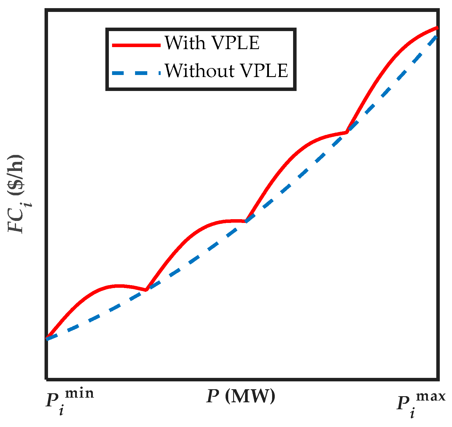
Figure 1. Operating cost with and without VPLEs.
Energies 16 04554 g001
Figure 2. Typical fuel cost function with VPLEs and three POZs.
Energies 16 04554 g002
Figure 3. Standard DE algorithm flowchart.
Energies 16 04554 g003
Figure 4. Bifurcation of the logistic map.
Energies 16 04554 g004
Figure 5. Convergence behaviors of the proposed ChMODE method for Case 1.
Energies 16 04554 g005
Figure 6. PF obtained by ChMODE for test system 1 ( P l d = 1200   MW ).
Energies 16 04554 g006
Figure 7. Convergence behaviors of the proposed ChMODE method for test system 2.
Energies 16 04554 g007
Figure 8. PF obtained by ChMODE for Case 2 ( P l d = 2000   MW ).
Energies 16 04554 g008
Figure 9. Comparison of convergence behaviors for Case 3. (a) EcDP case. (b) EmDP case.
Energies 16 04554 g009
Figure 10. PF of ChMODE and compromise solutions for Case 3.
Energies 16 04554 g010
Figure 11. The cost and emission boxplots for MODE and ChMODE algorithms.
Energies 16 04554 g011
Table 1. Classification of some metaheuristic techniques used for EcDP and EEDP.
MethodSwarm
Based
Social
Based
Biology
Based
Physics
Based
Math
Based
Chemistry
Based
Music
Based
Sports
Based
HybridSigle ObjectiveMulti Objective
PSO [12]
IHS [14]
QOCRO [27]
MBGSA [28]
LCA [29]
NSGA-III [24]
OWP-based OMF [30]
MOPSO [31]
IABC [32]
CSCA [5]
ACO-ABC-HS [33]
MTLSBA [3]
NSGAII [11]
Table 2. Setting parameters of the compared algorithms.
ChMODE and DE Parameters
Population size300
Maximum number of iterations200
CR0.75
F0.75
Mutation operatorDE/rand/1
Crossover operatorBinomial crossover
ABC parameters
Number of bees300
Number of food sources150
Maximum number of iterations200
Trial limit30
IWO parameters
Population size300
Maximum number of iterations200
Maximum number of seeds5
Minimum number of seeds0
Initial value of standard deviation2
Final value of standard deviation0.01
Table 3. EcDP for Case 1.
Unit Output (MW) QOTLBO [70]EMOCA [71]BSA [72]NSGA-III [29]DE [69]ChMODE
P1 (MW)79.554790.0079.676284.628584.435480.6856
P2 (MW)88.897788.0888.750793.421393.363887.5760
P3 (MW)210.0000210.00210.0000210.0000225.0000225.0000
P4 (MW)224.9944225.00225.0000225.0000209.9995210.0000
P5 (MW)324.9708315.00325.0000315.0000325.0000325.0000
P6 (MW)324.9977325.00324.9927325.0000314.9998325.0000
TC ($/h)63,97764,100.363,97664,09964,08363,963.96
TE (lb/h)1360.11345.731360.11345.91345.61359.87
Ptl (MW)53.4253.0853.4253.049852.798553.26
Table 4. EmDP for Case 1.
Unit Output (MW)QOTLBO [70]EMOCA [71]BSA [72]NSGA-III [29]DE [69]ChMODE
P1 (MW)125.0000125.00125.0000125.0000125.0000125.0000
P2 (MW)150.0000150.00150.0000150.0000150.0000150.0000
P3 (MW)201.2679201.26201.2684201.4824201.1816201.2684
P4 (MW)199.3701197.63199.369198.8723199.5454199.3690
P5 (MW)287.9708290.40287.9713288.5129287.6191287.9713
P6 (MW)286.5498285.83286.5499286.2913286.8137286.5499
TC ($/h)65,99265,985.665,99265,99265,99165,990.4
TE (lb/h)1240.61240.571240.61240.71240.71240.6
Ptl (MW)50.158650.1250.158650.158950.159850.1586
Table 5. BCSs for Case 1.
UnitQOTLBO [70]EMOCA [71]SSA-WSA [71]MODE [69]BSA [72]NSGA-III [29]ChMODE
P1 (MW)107.3101106.693107.0054108.6284104.0109107.9932105.4536
P2 (MW)121.4970115.6497116.6309115.9456117.4296118.3631118.7674
P3 (MW)206.5010210.0000206.8649206.7969207.5811210.0000210.0413
P4 (MW)206.5826203.3266205.7633210.0000206.6238204.6500203.2925
P5 (MW)304.9838303.0506309.3058301.8884309.0648306.6592308.5158
P6 (MW)304.6036313.0506305.2939308.4127306.9983303.8712305.5247
TC ($/h)64,91264,790.37064,819.16364,84364,766.82364,83064,815.143
TE (lb/h)12811288.9701287.47512861289.58612851286.563
Ptl (MW)51.5051.7750.8651.6751.7151.536751.60
Table 6. EcDP for Case 2.
UnitDE [69]QOTLBO [70]OWP-Based
OMF [30]
MOCDOA [31]NSGA-III [29]KSO [73]ChMODE
P1 (MW)55.000055.000055.000054.127155.000055.000055.0000
P2 (MW)79.806379.999180.000079.207680.000080.000080.0000
P3 (MW)106.8253107.9231106.877194.9232106.0514106.8407106.9399
P4 (MW)102.830798.6479100.702392.962899.2176100.9243100.5760
P5 (MW)82.241882.018081.53781.761381.580881.321081.5017
P6 (MW)80.435283.487882.9221110.961785.196482.945783.0212
P7 (MW)300.0000300.0000300.0000299.2531299.9843300.0000300.0000
P8 (MW)340.0000340.0000340.0000336.9639340.0000340.0000340.0000
P9 (MW)470.0000469.9706470.0000467.1387470.0000470.0000470.0000
P10 (MW)469.8975469.9988470.0000469.4260470.0000470.0000470.0000
TC ($/h)111,500111,498111,497.6407111,647.2433111,500111,497.27111,497.6308
TE (lb/h)4581.04568.74572.43964463.735545624573.244572.1944
Ptl (MW)87.036887.045387.038686.725487.030587.037487.0388
Δ P (MW)3.05 × 10−62.57 × 10−5NANANA5.68 × 10−30
Table 7. EmDP for Case 2.
UnitDE [69]QOTLBO [70]OWP-Based
OMF [30]
MOCDOA [31]NSGA-III [29]KSO [73]ChMODE
P1 (MW)55.000055.000055.000053.967655.000055.000055.0000
P2 (MW)80.000080.000080.000072.905979.978280.000080.0000
P3 (MW)80.592481.134280.924891.018282.128981.134281.1342
P4 (MW)81.023381.363781.101986.649082.350681.363781.3637
P5 (MW)160.0000160.0000160.0000159.9516160.0000160.0000160.0000
P6 (MW)240.0000240.0000240.0000238.7233240.0000240.0000240.0000
P7 (MW)292.7434294.4843294.5495276.9106296.1872294.4851294.4851
P8 (MW)299.1214297.2710297.6624298.1337296.2329297.2701297.2701
P9 (MW)394.5147396.7645396.3406389.5693397.4092396.7657396.7657
P10 (MW)398.6383395.5775396.0266413.7970392.2266395.5763395.5763
TC ($/h)116,400116,412.44116,411.9936116,322.8936116,430116,412.44116,412.4441
TE (lb/h)3932.43932.243932.25383950.76443932.53932.243932.2433
Ptl (MW)81.633581.595281.605781.626281.513681.595181.5952
Δ P (MW)9.04 × 10−54.07 × 10−5NANANA4.69 × 10−50
Table 8. Nondominated solutions with ChMODE (Case 2).
TC ($/h)116,393.2399114,826.3280115,599.7082112,797.543111,557.6631111,831.5004
TE (lb/h)3932.39504000.99183961.37454188.68164481.56754375.0299
Table 9. BCSs (Case 2).
UnitMODE [69]KSO [73]QOTLBO [70]BSA [72]OWP-Based
OMF [30]
MOCDOA [31]NSGA-III [29]ChMODE
P1 (MW)54.948755.000055.000055.000055.000053.019854.932455.0000
P2 (MW)74.582180.000080.000080.000080.000075.439780.000080.0000
P3 (MW)79.429484.741284.845785.646681.108589.556482.889386.0167
P4 (MW)80.687583.418583.499384.127080.772586.966383.783584.3972
P5 (MW)136.8551143.7777142.9210136.4905160.0000137.3076149.0664133.0681
P6 (MW)172.6393164.2877163.2711155.5642240.0000147.6495153.8082151.3739
P7 (MW)283.8233299.5076299.8066300.0000291.5934289.5841299.6631300.0000
P8 (MW)316.3407315.4369315.4388316.6807296.0321322.6523317.0490318.2507
P9 (MW)448.5923427.8255428.5084434.1352398.8523442.612435.7486436.8178
P10(MW)436.4287429.7994430.5524436.5834398.3150439.6483427.0254439.5055
TC ($/h)113,444.85113,505113,460113,126.7515116,391.8270112,729.353799113,410112,960.6297
TE (lb/h)4113.984105.6241104146.72863932.40354180.8688134118.64167.0660
Ptl (MW)83.5684.856383.843384.227681.679084.436083.965984.4299
Table 10. Statistical results for both EcDP and EmDP (Case 2).
MethodsEconomic DispatchEmission Dispatch
BestMeanWorstStdBestMeanWorstStd
ChMODE111,497.63111,497.63111,497.635.51 × 10−93932.243932.243932.249.39 × 10−12
SAIWPSO [63]111,497.63111,497.64111,497.641.81 × 10−43932.243932.253932.252.33 × 10−3
OWP-OMF [61]111,497.640111,497.64111,497.6423.9 × 10−43932.253932.25423932.2553.2 × 10−4
GQPSO [60]112,429.74113,102.46113,327.072.56 × 1024011.924032.934042.197.55 × 100
Table 11. POZs of the ten-unit system.
UnitPOZ1POZ2
P i , 1 D ( MW ) P i , 1 U ( MW ) P i , 2 D ( MW ) P i , 2 U ( MW )
112173545
220304045
990110240250
10150165448453
Table 12. Comparison of results for EcDP and EmDP (Case 3).
EcDPEmDP
UnitIWOABCDEChMODEIWOABCDEChMODE
P1 (MW)54.964455.00054.972655.000054.936755.000055.000055.0000
P2 (MW)69.777777.195580.000080.000079.409780.000080.000078.6128
P3 (MW)111.0655113.1760107.7073106.940079.161691.876380.456878.4628
P4 (MW)92.7977102.3596100.2584100.576378.639891.653779.504278.6725
P5 (MW)129.4502144.117881.081681.5017159.9894152.2381160.0000160.0000
P6 (MW)162.1251112.112383.326383.0209239.9808223.2139240.0000240.0000
P7 (MW)276.9582260.6269300.0000300.0000279.8024263.5496272.1162278.5313
P8 (MW)323.0147293.9795339.8291340.0000283.7445249.5820284.8455280.8442
P9 (MW)393.7317457.9211470.0000470.0000373.7658422.8764377.5210379.4409
P10 (MW)469.9996468.7058469.8573470.0000453.0547453.0631453.0478453.0000
TC ($/h)113,252.3886112,662.9052111,499.3218111,497.6308116,344.5128115,476.9771116,322.3313116,329.3508
TE (lb/h)4228.19944350.20474573.57534572.19583966.197084036.16523966.43473965.61212
Ptl (MW)83.884885.194687.032587.038882.485483.053282.491582.5644
Δ P (MW)00000000
Table 13. Statistical results for Case 3.
MethodsEconomic DispatchEmission Dispatch
BestMeanWorstStdBestMeanWorstStd
ChMODE111,497.63111,497.63111,497.634.27 × 10−53965.613965.613965.612.96 × 10−9
DE111,499.32111,507.60111,518.596.90 × 1003966.433977.574061.782.96 × 102
ABC112,662.91113,856.98114,851.368.82 × 1024036.174103.984200.687.02 × 102
IWO113,252.39113,426.98113,602.45 × 1023966.203967.263968.851.4 × 101
Table 14. Compromise solutions for Case 3.
UnitIWOABCDEChMODE
P1 (MW)55.000053.405155.000054.9645
P2 (MW)70.361677.317780.000079.9985
P3 (MW)83.663974.352983.831285.3545
P4 (MW)99.930269.574881.032283.9675
P5 (MW)123.7151132.0192147.3838130.8185
P6 (MW)214.5914164.1634169.8290149.2222
P7 (MW)276.0150291.2655289.6293298.5015
P8 (MW)268.1567333.5401307.7289315.4726
P9 (MW)438.8978435.9634416.4693433.4295
P10 (MW)453.3848453.3839453.1049453.0000
TC ($/h)114,505.3639113,217.4619113,678.6333112,846.3343
TE (lb/h)4115.13284173.30204098.36344184.4041
Ptl (MW)83.716584.986084.008784.7294
Δ P (MW)0000
Table 15. Performance indicators for Case 2.
ChMODEMODENSPSOMOCDOAMOPSONSGA-IIPESA-IIMOSSA
ASD0.68230.67560.67900.68020.65660.57300.6471NR
IGD0.45070.47250.4551NRNRNRNRNR
HV0.0330.0260.032NRNRNRNRBetween 0.024 and 0.027
SM0.95681.1266NRNRNRNRNRNR
Disclaimer/Publisher’s Note: The statements, opinions and data contained in all publications are solely those of the individual author(s) and contributor(s) and not of MDPI and/or the editor(s). MDPI and/or the editor(s) disclaim responsibility for any injury to people or property resulting from any ideas, methods, instructions or products referred to in the content.