Discussion on Operational Stability of Governor Turbine Hydraulic System Considering Effect of Power System

Abstract

Hydropower has grown to play an important role in power systems including increasing clean and low-carbon energies, and the effect of electric loads should be basically evaluated for the reliable operation of these systems. For the hydraulic–mechanical–electrical system of the hydropower station, the state equation model for stability evaluation was derived with typical electric load models and elastic models for pipe flow, and after experimental confirmation with a built single-unit setup for a system, the effects of different electrical loads and pipe flow models on typical hydropower systems stability were investigated in detail. The results indicate that for the built single-unit system with different load characteristics, the numerical results were basically consistent with experimental research, and the unit’s regulation performance for the dynamic load was superior to that of the static load. Evident differences existed in the effects of different electric loads on the operational stability, mainly depending on the pipe length and the corresponding models, and an optimum-order elastic model of pipe flow was preferred to reveal the dynamic interactions between different systems. Furthermore, for a typical two-unit system, the potential coupling resonance hydraulic–mechanical–electrical system is pointed out with the preferred-order elastic model of pipe flow.

1. Introduction

With the gradually growing energy demand, renewable and low-carbon energy sources have become a considerable part of the global energy mix [1]. Among them, for the utilization of water energy, many hydropower stations were successively constructed and brought into service, including the power transmission projects from west to east in China [2,3]. These hydropower stations are well suited to provide scheduling flexibility and play an important role in the normal operation of the power system after the grid connection [4,5,6,7,8]. Then, the stable operation of hydropower systems not only is beneficial to improve its power supply quality but also ensures reliable service of the parallel power system [9,10].

For the hydropower system, its normal operation and regulation is a dynamic process in which the governor turbine hydraulic system and the parallel power system inevitably have a dynamic interaction. During the generation condition of the hydropower system, as a consumer for water energy utilization, because the power system includes different electric loads, the effect of the power system on the operational stability of the governor turbine hydraulic system in the hydropower stations basically depends on the electric loads with different characteristics. Therefore, the assessment of different electric loads is indispensable to analyze the operational stability of the hydropower system [11]. Typically, two typical electric loads in power systems are often concerned, namely, the static load with basically unchanged impedance [12] and the dynamic load with quick response to frequency changes in dynamic studies [13]. Recently, the increasing complexity of new generation units and water systems has caused the load instability to become a new problem in many countries [14,15,16,17], mainly because of the complex interactions of hydro-mechanical power subsystems in the hydropower stations.

Hence, proper models of the electrical loads are the premise to understand their dynamic behaviors in different systems, and their importance in power system stability studies has been emphasized over the long term [18,19,20]. Relevant achievements have been obtained by numerical analysis in recent years. It has enabled researchers to further present the effect of load characteristic on the damping for low-frequency oscillation in the power system [21]. Similarly, the influence of different loads on the damping analysis of the power system was studied by numerical analysis [22]. In fact, the main motivation for the implementation of these load models is that static load models cannot predict instability in different subsystems. For instance, Nomikos analyzed the impact of a dynamic load, that is, an induction motor, on a mechanical–electrical oscillation in the power system and emphasized that the dynamic load had an evident impact on inter-area modes of power systems [23]. Hiskens and Milanović also studied the impact of these load models on the stability and analytical damping of the power system [24,25]. Their research shows that the recovery time constant of the dynamic load has a major effect on the eigenvalue analysis of the system.

Furthermore, alternative approaches are adopted based on the experimental setup and laboratory measurements instead of numerical simulation of the electrical loads. To investigate the dynamic stability of the governor turbine hydraulic system at a large hydropower station, Yang et al. carried out experimental research with simulated units [26]. Zeng et al. performed a full-load rejection test to confirm the effect of the S-shaped property on the water hammer calculation, which provided important experimental data to ensure the stable operation of the pumped storage station [27]. In addition, based on the physical model experiment, an analysis method considering the theoretical model was provided by Yang et al. [28], and the sustained ultra-low-frequency oscillations and frequency instability of hydropower units were revealed.

Worth noting is that the integration of pipe flow models and various electrical loads in hydropower systems remains a relatively unexplored research field. The effect analysis of load characteristics on operational stability has been preliminarily discussed in detail before [29], but it is still insufficient to meet the present demand or provide a comprehensive analysis of the influence mechanisms of different-order elastic models of pipe flow together with various electrical loads on typical hydropower systems. Most importantly, the load-influencing mechanism on the power system stability should be clarified in detail, in the case of complex load characteristics after the integration of the hydraulic–mechanical system with the power system. Therefore, further analysis with different load characteristics is urgent to ensure the system’s stable operation in different operating boundaries. After the mathematical model of the hydraulic–mechanical system is derived and organized, with further introduction of load models with different characteristics, the simulation model presented by state equations is derived to reveal the effects of different load characteristics on the system’s stability. Then, a built experiment setup of the hydraulic–mechanical–electrical system for a hydropower station [30] is also introduced for further confirmation analysis with numerical analysis. Finally, the effects of elastic models with different orders of pipe flow with different load characteristics on the system’s stability are investigated in detail based on two case analyses.

The rest of this paper is organized as follows. In Section 2, the mathematical models of static and dynamic loads are established in the form of state equations, together with the derived mathematical models of the governor turbine hydraulic system. In Section 3, the experimental-based stability study and confirmation of the numerical model are carried out through the experimental setup of hydro-mechanical power systems. In Section 4, based on a single-unit system and a two-unit system, the sensitivity analysis of the model order of pipe flow together with different load characteristics was conducted, followed by further numerical analysis. Finally, the conclusions are presented in Section 5.

2. Mathematical Models

For the hydropower station paralleled in the power system, its dynamic characteristics were mainly concerned with the hydraulic pipelines, the turbine generator, the governor, the exciter, and the electric loads. Therefore, in order to clarify the inherent dynamic interaction of the governor turbine hydraulic system and the power system and accurately reveal the effect of different pipe flow models and different electrical loads on the system’s operational stability, their mathematical models should be accurately established with the inter-variables.

2.1. Hydraulic System

For a simple hydropower system with a water diversion pipe and a hydraulic unit at the downstream end, different linear models, including rigid models and elastic models, can be deduced for the pipe flow provided in [31]. Then, as a single-unit system is considered, the state equations for state variables at the pipe’s outlet section are

$$\left\{\begin{array}{c}\frac{d{T}_i}{dt}=q_i\hfill \\ \frac{d{q}_i}{dt}=-\frac{f{Q}_0}{DA}{q}_i-\frac{{(i\pi a)}^2}{l^2}{T}_i-\frac{2gA{H}_0{(-1)}^i}{l}\xi \hfill \\ \frac{dq}{dt}=-\frac{f{Q}_0}{DA}q+\frac{1}{Q_0}{\displaystyle \sum _{i=1}^n\frac{{(i\pi a)}^2{(-1)}^i}{l^2}{T}_i}-\frac{H_0}{Q_0}\frac{(2n+1)gA}{l}\xi \end{array}\right.,$$

(1)

where q_i and T_i are the ith-order oscillatory flow rate and introduced conversion variable; l is the pipe length; f, D, A, and a are the pipe’s friction coefficient, diameter, sectional area, and wave speed, respectively; H₀ and Q₀ are the initial pressure and flow rate at the pipe’s end section of pressurized pipe; q and ξ are unit’s relative variation of flow rate and operating head; and n is the model order.

Here, based on the linearization of the turbine’s flow equations at a given operation condition [32], the unit’s relative variation of operating head in Equation (1) can be described by

$$\xi =C_{1}q+C_2\phi +C_3\mu ,$$

(2)

where φ and μ are unit’s relative variation of rotational speed and wicket opening, and C_i (i = 1, 2, 3) are parameters obtained from the model hill charts of the hydraulic turbine according to a given operating condition.

By the introduction of Equation (2), Equation (1) can be rewritten as follows:

$$\left\{\begin{array}{l}\frac{d{T}_i}{dt}=q_i\\ \frac{d{q}_i}{dt}=-\frac{f{Q}_0}{DA}{q}_i-\frac{(i\pi a{)}^2}{l^2}{T}_i-\frac{2gA{H}_0(-1{)}^i{C}_1}{l}q-\frac{2gA{H}_0(-1{)}^i{C}_2}{l}\phi -\frac{2gA{H}_0(-1{)}^i{C}_3}{l}\mu \\ \frac{dq}{dt}=\frac{1}{Q_0}{\displaystyle \sum _{i=1}^n\frac{{(i\pi a)}^2{(-1)}^i}{l^2}{T}_i}-\left(\frac{f{Q}_0}{DA}+\frac{H_0}{Q_0}\frac{(2n+1)gA{C}_1}{l}\right)q-\frac{H_0}{Q_0}\frac{(2n+1)gA{C}_2}{l}\phi -\frac{H_0}{Q_0}\frac{(2n+1)gA{C}_3}{l}\mu \end{array}\right.$$

(3)

Equation (3) is a typical state equation group mainly involving a different-order elastic model of pipe flow, which provides the dynamic interaction between the hydraulic system and the mechanical system with some inter-variables.

Similarly, for different hydropower systems, the elastic model can also be derived with state variables at the outlet section for the long water diversion pipelines connected to an upstream surge tank or bifurcation or with state variables at the inlet section for the tail pipelines introduced from a downstream surge tank or bifurcation.

2.2. Turbine Generator

For the turbine generator unit, as a typical salient pole generator, the commonly used stability computation model is the five order equations recommended by IEEE [33], which can exactly simulate its transient characteristics and dynamic responses and conveniently introduce the interaction of hydraulic–mechanical system. Its basic equations include

$$\frac{d{E}_q^{\prime }}{dt}=\frac{1}{T_{d0}^{\prime }}\left[E_{fd}-E_q^{\prime }-\left(x_d-x_d^{\prime }\right)i_d\right],$$

(4)

$$\frac{d{E}_q^{″}}{dt}=\left(\frac{1}{T_{d0}^{\prime \prime }}-\frac{1}{T_{d0}^{\prime }}\right)E_q^{\prime }-\frac{1}{T_{d0}^{″}}{E}_q^{″}-\left(\frac{x_d-x_d^{\prime }}{T_{d0}^{\prime }}+\frac{x_d{}^{\prime }-x_d^{\prime \prime }}{T_{d0}^{\prime \prime }}\right)i_d+\frac{1}{T_{d0}^{\prime }}{E}_{fd},$$

(5)

$$\frac{d{E}_d^{″}}{dt}=\frac{1}{T_{q0}^{″}}\left[-E_d^{″}+\left(x_q-x_q^{\prime \prime }\right)i_q\right],$$

(6)

$$\frac{d\omega }{dt}=\frac{1}{M}\left[P_m-P_e\right],$$

(7)

$$\frac{d\delta }{dt}=\omega {\omega }_0,$$

(8)

where T_d0′, T_d0″, and T_q0″ are all time constants corresponding to the d-axis and the q-axis; M is the unit’s inertia time constant; ω and δ are the rotor’s angular speed and power angle; E_q′, E_q″, and E_fd are the q-axis transient potential and sub-transient potential and excitation potential respectively; E_d″ is the d-axis sub-transient potential; x_d, x_d′, x_d″, and x_q, x_q″ are all known parameters corresponding to the d-axis and q-axis; i_d and i_q are the d-axis and q-axis current; V_d and V_q are d-axis and q-axis voltage, $V_q=E_q^{″}-x_d^{″}{i}_d$, $V_d=E_d^{″}+x_q^{″}{i}_q$; V_t is the terminal voltage, $V_t^2=V_q^2+V_d^2$; and P_m and P_e are the mechanical and electromagnetic power.

For the hydraulic turbine at a certain operating condition, based on the linearized equation of the unit’s output [32] and further introduction of Equation (2), the relative power variation corresponding to the mechanical power P_m in Equation (7) can be obtained as

$$p_m=C_{4}q+C_5\phi +C_6\mu ,$$

(9)

where P_m is the relative power variation, and C_i (i = 4, 5, 6) are parameters obtained from the model hill charts of the hydraulic turbine according to a given operating condition. Similarly, the relative power variation corresponding to the electromagnetic power P_e in Equation (7) can be derived according to electric loads with different characteristics.

2.3. Electric Load in Power System

The electric loads mainly include the static load, dynamic load, and integrated load. Because the integrated load has the dynamic characteristics combined with the static load and dynamic load, and in most cases, it is difficult to introduce an exact simulation model with defined transient parameters, for their effect analysis on the system’s operational stability, the static load and dynamic load model is typically emphasized. Further, the induction motor is the commonly used dynamic load in a power system, and its dynamic characteristics are basically represented by the transient of the induction motor.

Static Load. The description form for the static load model can be rewritten by simplification.

$$P_l=P_{l0}\left[a_p{\left(\frac{E_q^{″}}{E_{q0}^{″}}\right)}^2+b_p\left(\frac{E_q^{″}}{E_{q0}^{″}}\right)+c_p\right],$$

(10)

where coefficients a_p, b_p, and c_p meet a_p + b_p + c_p = 1; P_l and P_l0 are the transient and rated active power, respectively; and E_q0″ is the q-axis initial sub-transient potential. The specified characteristics of the static load can be described by different combinations of a_p, b_p, and c_p.

Then, with the introduction of the static load model and by the Newton–Raphson linearization, the relative power variation corresponding to electromagnetic power P_e in Equation (7) can also be derived and reorganized as below [29]:

$$p_e=k_e{e}_q^{″}+k_s\theta ,$$

(11)

where e_q″ is the q-axis relative sub-transient potential an θ is the generator’s rotor angle. The derived coefficients are defined as below:

$$k_e=\frac{V_t}{x_d^{″}}\sin {\theta }_0+\frac{P_{l0}}{E_{q0}^{″}}(2a_p+b_p), k_s=\frac{E_{q0}^{″}{V}_t}{x_d^{″}}\cos {\theta }_0+\frac{V_t^2(x_d^{″}-x_q^{″})}{x_d^{″}{x}_q^{″}}\cos (2{\theta }_0).$$

With the substitution of the mechanical power P_m, Equation (9), and the electromagnetic power P_e, Equation (11), and further linearization, the unit’s motion Equation (7) is rewritten into

$$\frac{d\phi }{dt}=\frac{1}{T_a}\left(C_{4}q+C_5\phi +C_6\mu -k_e{e}_q^{″}-k_s\theta \right),$$

(12)

where T_a is inertia time constant of the turbine generator.

Dynamic Load. In order to clearly reveal the effect of the dynamic load on the system’s operational stability with a simplified simulation model, considering an induction motor with absolutely symmetrical d- and q-axes, after ignoring its transient process and defining positive inflow of current, the obtained state equations for the dynamic load are as follows:

$$\frac{d{E}_{qe}^{\prime }}{dt}=-\frac{1}{T^{\prime }}{E}_{qe}^{\prime }+\frac{1}{T^{\prime }}(x-x^{\prime })i_{de}$$

(13)

$$\frac{d{E}_{de}^{\prime }}{dt}=-\frac{1}{T^{\prime }}{E}_{de}^{\prime }-\frac{1}{T^{\prime }}(x-x^{\prime })i_{qe}$$

(14)

$$\frac{ds}{dt}=\frac{1}{2M^{\prime }}(T_m-T_e),$$

(15)

where T′ is the time constant; E_qe′ and E_de′ are the transient potentials of the q- and d-axes, respectively; x and x′ are the reactance and transient reactance; i_de and i_qe are the q- and d-axis currents; s is the slip of the motor; M′ is the inertia time constant; T_e is the electromagnetic torque; and T_m is the mechanical torque. Then, based on the voltage equations, the electromagnetic power formula, and the interface models for the generator and the electric load, the relative power variation corresponding to electromagnetic power P_e can also be derived for the dynamic load [12].

2.4. Stability Analysis Based on State Equations

Therefore, for a simple hydropower system with a water diversion pipe and a hydraulic unit at the downstream end, by further introduction of the mathematical models for the exciter and speed governor provided in [33,34], the whole state equations group can be organized to directly describe the dynamic characteristic of the governor turbine hydraulic system and power system, and the corresponding matrix form is

$$\frac{d\mathit{X}}{dt}=\mathbf{A}\mathit{X}+\mathbf{B}\mathit{U},$$

(16)

where A is the coefficient matrix, X is the state vector, B is the input matrix, and U is the disturbance vector.

For this single-unit system, the derived state vector X with the static load in Equation (16) is

$$X={[T_1,q_1,\cdots ,T_n,q_n,q,\phi ,y,\mu ,x_I,x_D,u_a,u_f,e_{fd},e_q^{\prime },e_q^{″},e_d^{″},\theta ]}^T,$$

(17)

where y, x_I, and x_D are the governor’s state variables; u_a and u_f are the output voltage and exciting feedback voltage of the voltage regulator; e_fd is relative the exciting potential for the exciter; e_q′ is the q-axis relative transient potential; and e_d″ is the d-axis relative sub- transient potential.

Similarly, for this single-unit system, the derived state vector with the dynamic load in Equation (16) is

$$X={[T_1,q_1,\cdots ,T_n,q_n,q,\phi ,y,\mu ,x_I,x_D,u_a,u_f,e_{fd},e_q^{\prime },e_q^{″},e_d^{″},e_{qe}^{\prime },e_{de}^{\prime },s,{\theta }_{12},{\theta }_1]}^T,$$

(18)

where e_qe′ and e_de′ are the q- and d-axis relative transient potentials; θ₁₂ meets θ₁-θ₂; and θ₁ and θ₂ are the generator’s and the induction motor’s rotor angles respectively.

In particular, if the dynamic characteristics of the generator, exciter, and electrical load are not considered, the simplified state vector in Equation (16), which is commonly used in stability analysis on the governor turbine hydraulic system, is

$$X={[T_1,q_1,\cdots ,T_n,q_n,q,\phi ,y,\mu ,x_I,x_D]}^T,$$

(19)

With the obtained state vectors for different considerations, the corresponding linear state equations can be built to describe the dynamic characteristics of the hydropower system, and then the system’s operational stability with dynamic responses will be investigated under small disturbance. If different electric loads are involved with the state vectors presented in Equations (17) and (18), with further eigenvalue and sensitivity analysis, the influence of different-order elastic models of pipe flow and different load characteristics on the system’s operational stability can be revealed.

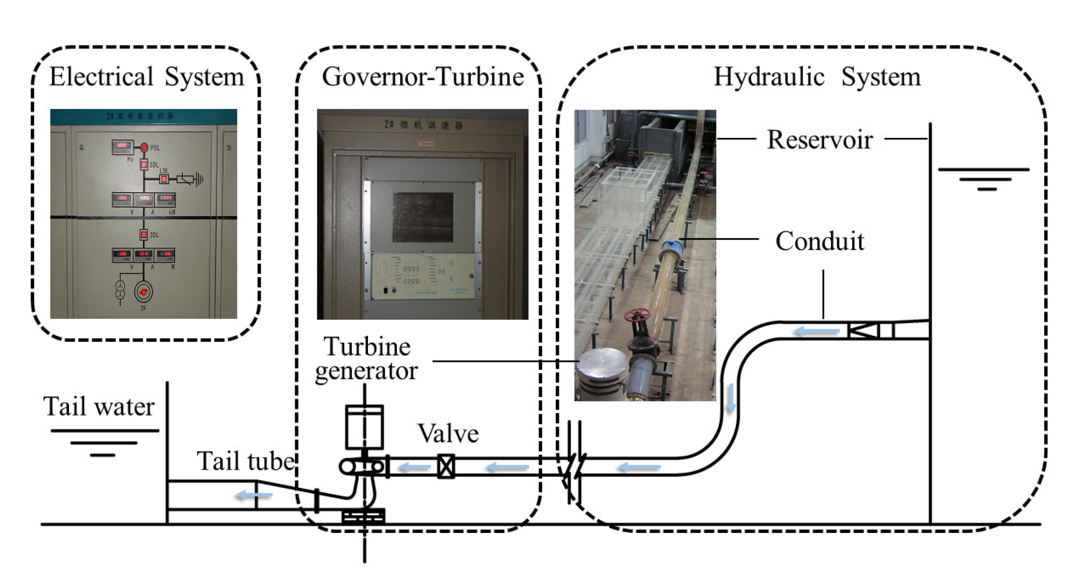
3. Experimental Research on System Stability

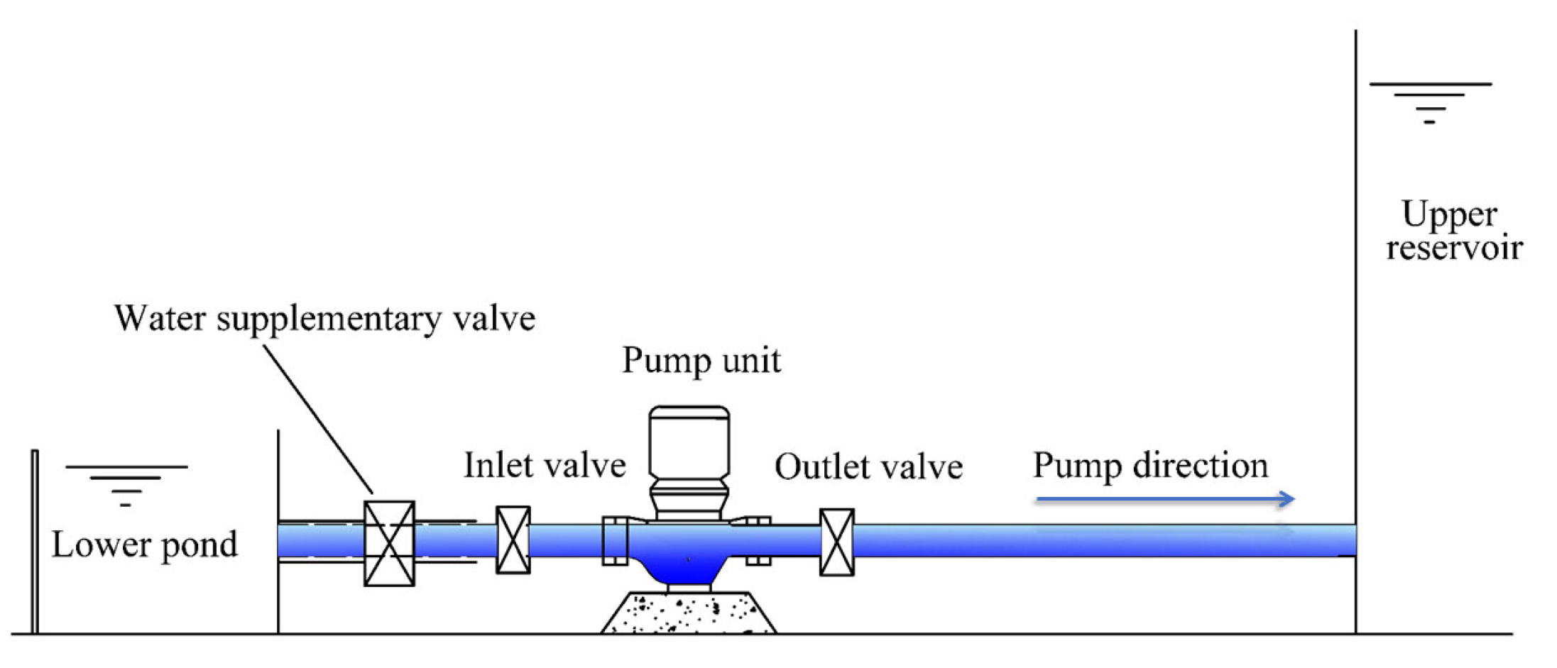
3.1. Experimental Setup

Considering the detailed layout of a given simple hydropower system, a small-scale experimental setup focusing on operating stability of the hydro-mechanical–electrical system was designed and established [30]. This equipment mainly consisted of an upstream reservoir, a pressure conduit, turbine generator, a tail tube, a governor, an exciter, a simplified electrical system, and so on, shown in Figure 1, and a short open channel was used to induce water flow from unit’s draft tube to the tail water. The total length of the water diversion conduit was 18.0 m with a 22.5 cm diameter, and the other experimental equipment parameters are shown in Appendix A. An electromagnetic flowmeter was set close to the inlet of the unit’s spiral case for the measurement of the unit’s operating flow rate.

The simulated hydropower system can be completely monitored under stable operation, normal starting and stopping, emergency load rejection, and small disturbances. The pressure sensors are preset at the corresponding sections to collect the real-time data of the simulated hydraulic system. With the equipped speed governor, exciter, and synchronization system, the simulated hydropower system can be synchronized and paralleled into the external power system or be put into isolated operation with different electric loads.

3.2. Electric Load Design

Considering to the research achievements on electric loads’ models in recent years [25], by comparing with the static load and dynamic load, there is still a bottleneck on how to ascertain the integrated loads and their parameters in the stability analysis.

Therefore, in order to clearly reveal the influence of the electric loads with different characteristics on the system’s stability, the static load and dynamic load were preferred instead of the integrated loads to realize the system’s stability evaluation. As an additional and indispensable part for the simulated hydropower system, the physical models were designed and established for the static load (electric resistance) and the dynamic load, which is a water pumping system with a three-phase induction motor [30] shown in Figure 2.

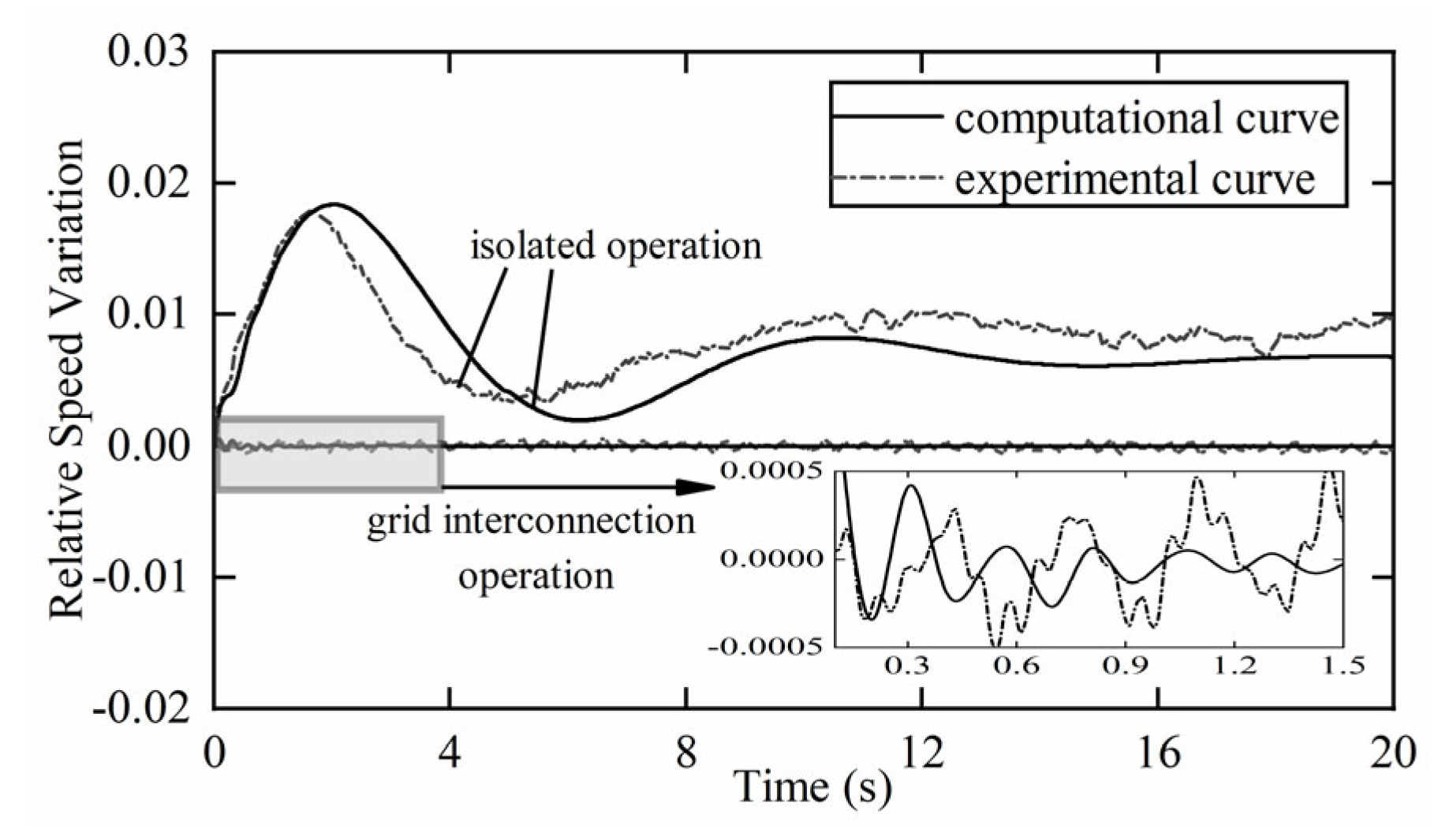
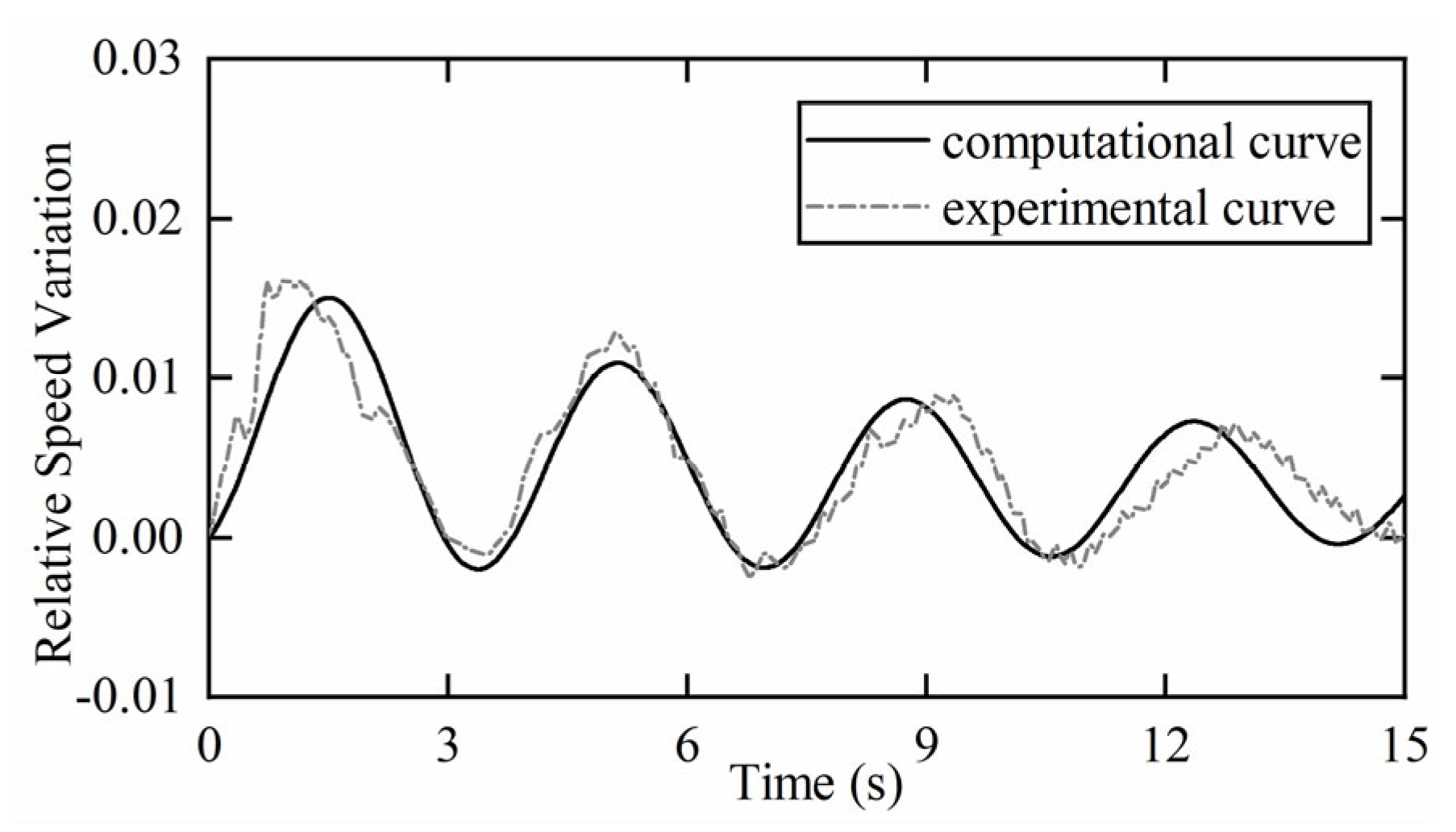
3.3. Computational Verification Based on the Simulated System

Based on the simulated hydropower system in Figure 1 running with rated head H_r = 3.2 m, rated flow rate Q_r = 0.045 m³/s, and rated rotational speed n_r = 600 rpm and then serving for different loads in Figure 2 paralleled into the external power system, considering electrical loads with different characteristics under grid-connected operation or isolated operation, the effect of power system and different load characteristics on system’s operational stability was experimentally studied. Then, for the simulated hydropower system, further numerical simulation was investigated on the system’s operational stability, and verification analysis for the numerical simulation was also conducted by comparative analysis with the experimental results [29].

For the simulated hydropower system in Figure 1 and Figure 2, under grid-connected operation or isolated operation with the static load or dynamic load, according to its relatively short pipe length, the rigid model was preferred to simulate the dynamic characteristics of pipe flow [31] instead of the elastic model, derived from Equation (3). Based on the derived state equations for the hydropower system with a state vector (17) for the static load and a state vector (18) for the dynamic load, respectively, with eigenvalue analysis and load disturbance computation, the effects of different load characteristics on the system’s stability and regulation performance could be numerically analyzed, including a comparative analysis with experimental results. For the simulated hydropower system, in order to be basically consistent with the experimental boundaries, for the static load, only resistance with a_p = 1 and b_p = 0 was concerned for the numerical computation, so based on the eigenvalue computation and further correlation analysis, the computed oscillation mode strongly related with the low-frequency oscillation was −0.0761 ± j2.041 for the static load (resistance), and it was −0.2492 ± j0.724 for the dynamic load. By a comparative analysis on the attenuation factor (real part of low-frequency oscillation mode) for different loads, it was revealed that the unit serving for a water pumping system (dynamic load) was more stable.

Considering the unit under grid interconnection operation and isolated operation and then with −10% step load disturbance, time histories of the unit’s relative speed variation considering the dynamic load for further comparative analysis with the experimental results are provided in Figure 3.

From the dynamic characteristics of the unit’s rotational frequency in Figure 3 under −10% step load disturbance considering grid-connected operation, it was obviously confirmed that the power system was beneficial to the unit’s stable operation. Because the simulated unit’s capacity had a very small proportion of the external power system, the electric load with different characteristics had a negligible influence on the system’s stability. As far as isolated operation was concerned, Figure 3 shows the similar oscillation trend and approximately equal peak values for numerical simulation and experimental research, and there was also some difference in the oscillation period and the attenuation trend, which was basically originated from the calibration error of the dynamic load’s technical parameters, such as the time constant, besides the experimental error.

Similarly, under a −10% step load disturbance, considering the unit under isolated operation, time histories of the unit’s relative speed variation considering the static load for further comparative analysis with the experimental results are shown in Figure 4.

From Figure 3 and Figure 4 and further unit regulation performance analysis, it can be drawn that, with setting parameters, under load disturbance, the unit serving for different loads under isolated operation was stable. For the unit serving for a water pumping system (dynamic load), the system’s stability and regulation performance were better than those of resistance (static load), including an obviously shorter regulating time, less oscillation, and a larger attenuation degree, which was 84.8% greater than that of the static load, 24.8%, well in agreement with the above experimental results.

Furthermore, Figure 3 and Figure 4 also clarify that the numerical computed curves were basically identical to the experimental results, which confirms that the established mathematical models can accurately reveal the system’s dynamic characteristics and the effects of different loads on the hydropower system stability performance.

4. Numerical Analysis

4.1. Case Description for a Simple Hydropower System

Considering that the unit’s speed was an important inter-variable for the governor turbine hydraulic system and the power system, for further numerical simulation analysis, it was preferable to investigate the effect of different electric loads on the dynamic characteristics of the unit’s speed in detail.

Figure 5 shows a simple hydropower system with a pressurized pipe 250 m in length and 5.0 m in diameter, and the unit’s rotational inertia is 11,000 t·m² with rated speed of 150.0 rpm. It was running with an operating head of 73.0 m and a flow rate of 116.0 m³/s.

4.2. Further Numerical Analysis with Different Loads

For the hydropower system shown in Figure 5, the first-order elastic model derived from Equation (3) was introduced to simulate the water flow in the diversion pipe according to its relatively short length. In order to reveal the effects of the dynamic characteristics of the generator, the exciter, and the electrical load on system’s stability, first, based on the state vector, Equation (19), without the consideration of their effects, the stable region is shown in Figure 6a with the governor parameters, including the dashpot time constant T_d and the temporary speed drop b_t. In Figure 6a, a critical combination of the governor parameters (T_d, b_t) is also provided for further comparative analysis, and then its corresponding computational curve of the relative speed variation under a −10% step load disturbance is yielded in Figure 6b.

Figure 6 illustrates that if the effect of the dynamic characteristic of the generator, excitor, and electrical loads on the system’s stability was not considered, the T_d-b_t plane was divided into a stable region and an unstable region with a critical curve; if the combination of the governor’s parameters (T_d, b_t) was just located along the critical curve, the system’s dynamic variables, mainly including relative speed variation, tended to equal-amplitude oscillation.

Furthermore, the effect analysis of the load characteristics on low-frequency oscillation was conducted based on the dynamic characteristics of the unit’s speed considering the static load or the dynamic load.

Table 1. Low-frequency oscillation mode of different load characteristics.

Load Model		ap	bp	2 ap + bp	Low-Frequency Oscillation Mode
					Td = 5.0 s, bt = 0.50	Td = 5.0 s, bt = 0.32
Static load	Constant resistance	1.0	0.0	2.0	−0.4316 ± j12.94	−0.4017 ± j12.94
	Constant current	0.0	1.0	1.0	−0.4005 ± j13.02	−0.3723 ± j13.01
	Constant output	0.0	0.0	0.0	−0.3697 ± j13.09	−0.3431 ± j13.08
		0.6	0.2	1.4	−0.4129 ± j12.99	−0.3840 ± j12.98
Dynamic load					−0.5599 ± j12.50	−0.5198 ± j12.54

provides various groups of a_p and b_p values to describe different computational cases considering the static load in addition to the dynamic load and the computed corresponding low-frequency oscillation modes. In Table 1, based on the sensitivity analysis of the governor’s parameters, the effects of governor parameters on the low-frequency oscillation mode is also analyzed, including the obtained critical combination of the governor parameters (T_d, b_t) in Figure 6.

It can be drawn from Table 1 that if the first-order elastic model of the pipe flow was introduced, the absolute value of the attenuation factor considering the dynamic load was obviously greater than that considering the static load. The absolute value of the attenuation factor increased, and the system’s stability became better as the value of 2 a_p + b_p for the static load was larger; considering the decreasing of b_t with the same T_d, the absolute value of the attenuation factor was slightly reduced, and its stability became a bit worse.

As the hydropower station was running and serving for the dynamic load or the static load (constant resistance), respectively, then by introducing a −10% step disturbance from the governor side, the time histories of the relative speed variations under isolated operation are shown in Figure 7 with T_d = 5.0 s and b_t = 0.50. Meanwhile, Figure 8 shows the time histories of the relative speed variation under a −10% step load disturbance with T_d = 5.0 s and b_t = 0.32 for further comparative analysis.

From Figure 7 and Figure 8, the dynamic process of the hydraulic–mechanical system was significantly different considering the influence of the static load or the dynamic load. At the same time, considering the dynamic load, the system’s operational stability was better with the faster speed fluctuation attenuation and relatively short regulation time as compared with the static load, which was consistent with the results in Table 1. From further comprehensive analysis with Figure 7 and Figure 8, there were obviously different behaviors for different disturbances from the governor side or the load disturbance, including different oscillation processed and attenuation rates. By comparative analysis with Figure 7 and Figure 8, with the same combination of the governor’s parameters (T_d, b_t), that is, T_d = 5.0 s and b_t = 0.32, the system was stable with better regulation performance considering the effects of the dynamic characteristics of the generator, exciter, and electrical loads, while it was in a critical state with equal-amplitude oscillation without their effects; therefore, it was concluded that the dynamic characteristics of the generator, exciter, and electrical loads could improve the system’s stability and regulation performance.

4.3. Effect of Pipe Flow Models on Low-Frequency Oscillation with Different Loads

In the above numerical analysis, the first-order elastic model for pipe flow was introduced to evaluate the effect of load characteristics on low-frequency oscillation and further the system’s stability. Furthermore, for the simple unit system shown in Figure 5, considering the detailed hydraulic characteristics of the pipe flow illustrated by different-order elastic models, that is, the stiff model, the first-order model, the second-order model, and the third-order model, which can be derived from Equation (1) with n = 0, 1, 2, and 3, respectively, the eigenvalue computation and the analysis of further dynamic characteristics was carried out to reveal the effects of different models of pipe flow on low-frequency oscillation and the system’s stability, together with the effect analysis of different load characteristics. The corresponding modes for low-frequency oscillation with different-order elastic models for pipe flow and different load characteristics are provided in

Table 2. Low-frequency oscillation modes of different-order elastic models for pipe flow.

Flow Model	Static Load	Dynamic Load
Stiff model (zeroth-order)	−0.5411 ± j12.80	−0.5036 ± j12.31
First-order elastic model	−0.4316 ± j12.94	−0.5599 ± j12.50
Second-order elastic model	−0.4278 ± j12.95	−0.5695 ± j12.50
Third-order elastic model	−0.4264 ± j12.95	−0.5735 ± j12.49

, and considering the static load, under a −10% step load disturbance, the dynamic curves of the relative speed variation are shown in Figure 9.

From Table 2 and Figure 9, it can be seen that for the static load, with the increasing of the model order for the pipe flow, the absolute value of the attenuation factor of the low-frequency oscillation mode gradually reduced and then tended to be a constant, which was illustrated by the different attenuation ratios for the relative speed variation. Compared with the static load (constant resistance), for dynamic loads, with the increasing of the model order for the pipe flow, the absolute value of the attenuation factor of the low-frequency oscillation mode gradually increased and then tended to be a constant. Therefore, for both the static load and the dynamic load, instead of a higher-order elastic model, an optimum-order elastic model, a three-order elastic model, of the pipe flow was preferred to exactly evaluate the effects of different load characteristics on the low-frequency oscillation mode and the system’s regulation performance.

4.4. Sensitivity Analysis of Pipe Length on Low-Frequency Oscillation with Different Loads

Based on the effect analysis of the pipe flow models on low-frequency oscillation with different loads, it was also necessary to conduct further sensitivity analyses of the pipe length on low-frequency oscillation. For the simple unit system in Figure 5, considering the reasonable change of the pipe length from 150 to 400 m, further sensitivity analysis was implemented focusing on the effect of the pipe length on low-frequency oscillation and further the system’s stability, along with different models of the pipe flow and different load characteristics. Based on detailed eigenvalue computation with different pipe lengths, the corresponding modes for low-frequency oscillation with different-order elastic models for the pipe flow and the static load (constant resistance) are provided in

Table 3. Low-frequency oscillation mode of different pipe length with static load.

Flow Model	150 m Pipe	250 m Pipe	400 m Pipe
Stiff model (zeroth-order)	−0.5347 ± j12.80	−0.5411 ± j12.80	−0.5447 ± j12.80
First-order elastic model	−0.5537 ± j12.79	−0.4316 ± j12.94	−0.5258 ± j12.80
Second-order elastic model	−0.5571 ± j12.80	−0.4278 ± j12.95	−0.5483 ± j12.79
Third-order elastic model	−0.5585 ± j12.80	−0.4264 ± j12.95	−0.5539 ± j12.79

, and the changing trends for the real part of the low-frequency oscillation mode of different pipe lengths with the dynamic load are shown in Figure 10.

It can be analyzed from Table 3 and Figure 10 that for both the static load and the dynamic load, if the stiff model of the pipe flow was introduced, the absolute value of the real part of the low-frequency oscillation mode slightly increased with the increasing pipe length. With the increasing model order for the pipe flow, considering different pipe lengths, the absolute value of the real part of the low-frequency oscillation mode followed a different variation tendency, and then all tended to be a constant. Therefore, in order to completely evaluate the effects of different load characteristics on the low-frequency oscillation mode, an optimum-order elastic model of the pipe flow was preferred according to different pipe lengths, and in this case, the first- to second-order elastic model would exactly reveal the effects of the pipe flow characteristics on the system’s regulation performance.

4.5. Discussion on Stability for Two-Unit System with Different Static Loads

In recent years, many hydropower stations have been successively constructed, paralleled into different power systems, and served for local power supply, which has strongly advanced the clean, low-carbon energy utilization and development in the world. Besides the simple unit hydropower systems, some typical and relatively complex hydropower systems play an important role in these hydropower systems, including the two-unit system sharing a common water diversion pipeline or tail tunnel with the necessary surge chambers. Therefore, Figure 11 shows a two-unit system sharing a downstream surge chamber and tail tunnel, with a water level in the reservoir of 150 m, a tail water level of 29.0 m, a sectional area of downstream surge tank of 233.4 m², a unit output of 122.6 MW, a unit rotational inertia of 8900 t·m², and a rated speed of 230.8 rpm. For the pipe parameters, the water diversion pipes were 466.3 m and 450.3 m in length with 5.7 m in diameter, the tail branches were 101.1 m and 111.1 m in length with 6.2 m in diameter, and the tail tunnel was 945.9 m in length and 8.8 m in diameter.

Considering two units in Figure 11 serving for the static load and by introducing different-order models for the tail tunnel flow and stiff models for the branch pipes, a detailed eigenvalue computation and analysis of further dynamic characteristics was carried out to discuss the effects of different models of pipe flow on low-frequency oscillation and the system’s stability, together with the effect analysis of different load characteristics. The corresponding modes for low-frequency oscillation and hydraulic oscillation with third-order elastic models for tail tunnel flow and different load characteristics are provided in

Table 4. Oscillation mode analysis with third-order elastic models for tail tunnel flow.

Oscillation Modes	Static Load (Constant Output)	Static Load (Constant Resistance)
Low-frequency oscillation	−0.9480 ± j6.834	−0.9569 ± j6.838
	−0.8839 ± j6.693	−1.1060 ± j5.471
Hydraulic oscillation	−0.005636 ± j3.322	−0.005365 ± j3.322
	−0.005635 ± j6.643	−0.005632 ± j6.643
	−0.005627 ± j9.964	−0.005637 ± j9.964
Water level oscillation	−0.008115 ± j0.5201	−0.008112 ± j0.5202

. Based on constant resistance, considering a −10% step load disturbance with a 1# unit, the dynamic curves of the relative state variables are shown in Figure 12, including the unit’s relative speed variation, the relative water level variation in the surge tank, and the oscillating flow rates in the tail tunnel.

From Table 4 and Figure 12, it can be concluded that for the two-unit system sharing a downstream surge tank and tail tunnel, if the third-order elastic model for the tail tunnel flow was introduced, the system’s oscillation modes mainly included two low-frequency oscillations modes strongly related with the two units, three hydraulic oscillation modes illustrating the dynamic characteristics of three oscillating flow rates, and one water level oscillation mode directly representing the downstream surge tank’s surge characteristics. The two low-frequency oscillation modes were not changed with the different model orders for the tail tunnel flow, mainly because of the reflection of the downstream surge tank, which was obviously different from that of the simple unit system. By comparative analysis, one of the low-frequency oscillation modes was basically consistent with one of the hydraulic oscillation modes, which may have resulted in coupling resonance in this hydropower system, which should be exactly evaluated with the premise of considering a reasonable model order for the tail tunnel flow.

Under a −10% load disturbance on a 1# unit, the detailed computation shows that the relative speed variation of the 1# unit decayed accompanied by obvious oscillation, while that of the 2# unit had less oscillation. The water level in the downstream surge tank also tended to a steady state gradually. Especially in Figure 12c, three oscillating flow rates q_i (i = 1, 2, and 3) showed an attenuated oscillation close to the water level oscillation period in the surge tank, combined with a high-frequency oscillation with an oscillation period decided by the ith-order hydraulic oscillation.

Further, considering static loads with different characteristics, from constant output to constant resistance, the absolute value of the real part of the low-frequency oscillation mode increased, and the relative speed variation decayed faster, while there was less effect on the hydraulic oscillation mode and the water level oscillation.

Therefore, similar to the single-unit system, for the typical two-unit system, the different characteristics of the electric loads also had obvious effects on the system’s operational stability, especially low-frequency oscillation, while the higher-order elastic model of the tail tunnel flow had no effect on low-frequency oscillation but revealed the potential coupling resonance between the hydraulic system and the power system.

5. Conclusions

After introducing the elastic model with a reasonable order for the pipe flow and the linear models of the hydro-mechanical–electrical system of the hydropower stations, the analytical model considering the electric loads with different characteristics was comprehensively derived with state equations. Further, based on the numerical simulation model confirmed by an experimental setup of a single-unit hydropower system, the effects of load characteristics and pipe flow models on the operational stability were investigated in detail, and the following can be concluded.

For a given single-unit hydropower system running with different electrical loads, if a first-order elastic model of the pipe flow is introduced, the system’s stability and the regulation performance of the unit running with the dynamic load under isolated operation was superior to that of the unit running with different static loads. Based on the stable region and sensitivity analysis of the governor’s parameters, it was confirmed that the dynamic characteristics of the generator, excitor, and electrical loads could improve the system’s stability and regulation performance.

Based on the influence analysis of different load characteristics on the single-unit hydropower system, it was pointed out that a relatively higher-order elastic model could exactly represent the dynamic characteristics of the pipe flow, while an optimum-order elastic model of the pipe flow according to different pipe lengths was preferred to evaluate the effects of different load characteristics on the low-frequency oscillation mode and the system’s regulation performance.

For a typical two-unit system, the load characteristics also had obvious effects on low-frequency oscillation, the low-frequency oscillation modes were not changed with the different model orders for the tail tunnel flow mainly because of the reflection of the downstream surge tank compared with the single-unit system, and considering the preferred-order model of the pipe flow, the possible coupling resonance between the hydraulic system and the power system could be exactly evaluated.

References

1. Zhang, D.; Wang, J.; Lin, Y.; Si, Y.; Huang, C.; Yang, J.; Huang, B.; Li, W. Present situation and future prospect of renewable energy in China. Renew. Sustain. Energy Rev. 2017, 76, 865–871. [Google Scholar] [CrossRef]
2. Chang, X.; Liu, X.; Zhou, W. Hydropower in China at present and its further development. Energy 2010, 35, 4400–4406. [Google Scholar] [CrossRef]
3. Zhang, L.; Wu, Q.; Ma, Z.; Wang, X. Transient vibration analysis of unit-plant structure for hydropower station in sudden load increasing process. Mech. Syst. Sig. Process. 2019, 120, 486–504. [Google Scholar] [CrossRef]
4. Hamann, A.; Hug, G.; Rosinski, S. Real-Time Optimization of the Mid-Columbia Hydropower System. IEEE Trans. Power Syst. 2017, 32, 157–165. [Google Scholar] [CrossRef]
5. Xu, B.; Zhang, J.; Egusquiza, M.; Chen, D.; Li, F.; Behrens, P.; Egusquiza, E. A review of dynamic models and stability analysis for a hydro-turbine governing system. Renew. Sustain. Energy Rev. 2021, 144, 110880. [Google Scholar] [CrossRef]
6. Xu, J.; Ni, T.; Zheng, B. Hydropower development trends from a technological paradigm perspective. Energy Convers. Manag. 2015, 90, 195–206. [Google Scholar] [CrossRef]
7. Yu, X.; Zhang, J.; Fan, C.; Chen, S. Stability analysis of governor-turbine-hydraulic system by state space method and graph theory. Energy 2016, 114, 613–622. [Google Scholar] [CrossRef]
8. Yu, X.D.; Zhou, Q.; Zhang, L.; Zhang, J. Hydraulic Disturbance in Multiturbine Hydraulically Coupled Systems of Hydropower Plants Caused by Load Variation. J. Hydraul. Eng. 2019, 145, 04018078. [Google Scholar] [CrossRef]
9. Cassano, S.; Sossan, F. Model predictive control for a medium-head hydropower plant hybridized with battery energy storage to reduce penstock fatigue. Electr. Power Syst. Res. 2022, 213, 108545. [Google Scholar] [CrossRef]
10. Reigstad, T.I.; Uhlen, K. Optimized Control of Variable Speed Hydropower for Provision of Fast Frequency Reserves. Electr. Power Syst. Res. 2020, 189, 106668. [Google Scholar] [CrossRef]
11. Makarov, Y.V.; Maslennikov, V.A.; Hill, D.J. Revealing loads having the biggest influence on power system small disturbance stability. IEEE Trans. Power Syst. 1996, 11, 2018–2023. [Google Scholar] [CrossRef]
12. Kundur, P. Power System Stability and Control; McGraw-Hill Professional: New York, NY, USA, 1994; pp. 377–417. [Google Scholar]
13. Garmroodi, M.; Hill, D.J.; Verbic, G.; Ma, J. Impact of Load Dynamics on Electromechanical Oscillations of Power Systems. IEEE Trans. Power Syst. 2018, 33, 6611–6620. [Google Scholar] [CrossRef]
14. Jiang, C.X.; Zhou, J.H.; Shi, P.; Huang, W.; Gan, D.Q. Ultra-low frequency oscillation analysis and robust fixed order control design. Int. J. Electr. Power Energy Syst. 2019, 104, 269–278. [Google Scholar] [CrossRef]
15. Mo, W.; Chen, Y.; Chen, H.; Liu, Y.; Zhang, Y.; Hou, J.; Gao, Q.; Li, C. Analysis and Measures of Ultra-Low-Frequency Oscillations in a Large-Scale Hydropower Transmission System. IEEE J. Emerg. Sel. Top. Power Electron. 2017, 6, 1077–1085. [Google Scholar] [CrossRef]
16. Villegas Pico, H.; Mccalley, J.D.; Angel, A.; Leon, R.; Castrillon, N.J. Analysis of Very Low Frequency Oscillations in Hydro-Dominant Power Systems Using Multi-Unit Modeling. IEEE Trans. Power Syst. 2012, 27, 1906–1915. [Google Scholar] [CrossRef]
17. Wang, G.; Zheng, X.; Guo, X.; Liang, X. Mechanism analysis and suppression method of ultra-low-frequency oscillations caused by hydropower units. Int. J. Electr. Power Energy Syst. 2018, 103, 102–114. [Google Scholar] [CrossRef]
18. Li, Y.; Chiang, H.D.; Choi, B.K.; Chen, Y.T.; Huang, D.H.; Lauby, M.G. Load models for modeling dynamic behaviors of reactive loads: Evaluation and comparison. Int. J. Electr. Power Energy Syst. 2008, 30, 497–503. [Google Scholar] [CrossRef]
19. Maslennikov, V.A.; Milanovic, J.V.; Ustinov, S.M. Robust ranking of loads by using sensitivity factors and limited number of points from a hyperspace of uncertain parameters. IEEE Trans. Power Syst. 2002, 22, 565–570. [Google Scholar] [CrossRef]
20. Price, A.W.W.; Taylor, C.W.; Rogers, G.J. Bibliography on load models for power flow and dynamic performance simulation. IEEE Trans. Power Syst. 1995, 10, 523–538. [Google Scholar] [CrossRef]
21. Yang, Y.; Zhao, S.Q. Load characteristics’ effect on low-frequency oscillation damping of power systems. Electr. Power Autom. Equip. 2003, 23, 13–16. [Google Scholar] [CrossRef]
22. Kao, W.S. The effect of load models on unstable low-frequency oscillation damping in taipower system experience w/wo power system stabilizers. IEEE Trans. Power Syst. 2001, 16, 463–472. [Google Scholar] [CrossRef]
23. Nomikos, B.M.; Vournas, C.D. Evaluation of motor effects on the electromechanical oscillations of multimachine systems. In Proceedings of the 2003 IEEE Bologna Power Tech Conference, Bologna, Italy, 23–26 June 2003. [Google Scholar] [CrossRef]
24. Hiskens, I.A.; Milanovic, J.V. Load modelling in studies of power system damping. IEEE Trans. Power Syst. 1995, 10, 1781–1788. [Google Scholar] [CrossRef]
25. Milanovic, J.V.; Hiskens, I.A. Effects of load dynamics on power system damping. IEEE Trans. Power Syst. 1995, 10, 1022–1028. [Google Scholar] [CrossRef]
26. Yang, J.; Li, J.; Wang, D.; Chen, J.; Wu, R. Study on the physical simulation of transient process in conduits of hydropower stations. J. Hydroelectr. Eng. 2004, 23, 57–63. [Google Scholar]
27. Zeng, W.; Yang, J.; Hu, J. Pumped storage system model and experimental investigations on S-induced issues during transients. Mech. Syst. Sig. Process. 2017, 90, 350–364. [Google Scholar] [CrossRef]
28. Yang, W.; Yang, J.; Zeng, W.; Tang, R.; Hou, L.; Ma, A.; Zhao, Z.; Peng, Y. Experimental investigation of theoretical stability regions for ultra-low frequency oscillations of hydropower generating systems. Energy 2019, 186, 115816. [Google Scholar] [CrossRef]
29. Zhou, J.; Chen, G. Effect Analysis of Load Characteristic on Operation Stability of Hydropower Stations. In Proceedings of the 2012 International Conference on Future Electrical Power and Energy Systems, Sanya, China, 21–22 February 2012. [Google Scholar] [CrossRef]
30. Zhou, J.; Hu, M.; Cai, F.; Hu, R. Experimental Research on Stability of Hydro-Mechanical-Electrical System in Hydropower Station. In Proceedings of the 2009 Asia-Pacific Power and Energy Engineering Conference, New York, NY, USA, 28–30 March 2009. [Google Scholar] [CrossRef]
31. Zhou, J.; Cai, F.; Wang, Y. New Elastic Model of Pipe Flow for Stability Analysis of the Governor-Turbine-Hydraulic System. J. Hydraul. Eng. 2011, 137, 1238–1247. [Google Scholar] [CrossRef]
32. Zhou, J.X.; Mao, Y.T.; Shen, A.L.; Zhang, J. Modeling and stability investigation on the governor-turbine-hydraulic system with a ceiling-sloping tail tunnel. Renew. Energy 2023, 204, 812–822. [Google Scholar] [CrossRef]
33. Jaeger, E.D.; Janssens, N. Hydro turbine model for system dynamic studies. IEEE Trans. Power Syst. 1994, 9, 1709–1715. [Google Scholar] [CrossRef]
34. Hannett, L.N.; Feltes, J.W.; Fardanesh, B. Field tests to validate hydro turbine-governor model structure and parameters. IEEE Trans. Power Syst. 1994, 9, 1744–1751. [Google Scholar] [CrossRef]
Figure 1. Longitudinal section of the simulated hydro-mechanical system.
Energies 16 04459 g001
Figure 2. Longitudinal plan of the pumping system.
Energies 16 04459 g002
Figure 3. Time histories of the unit’s relative speed variation considering dynamic load.
Energies 16 04459 g003
Figure 4. Time histories of unit’s relative speed variation considering static load.
Energies 16 04459 g004
Figure 5. Sketch of a single-pipe and single-unit system.
Energies 16 04459 g005
Figure 6. Stability analysis without the effect of electrical system: (a) Stable region. (b) Relative speed variation.
Energies 16 04459 g006
Figure 7. Computational curves of unit’s relative speed variation under isolated operation.
Energies 16 04459 g007
Figure 8. Computational curves of relative speed variation under −10% step load disturbance.
Energies 16 04459 g008
Figure 9. Dynamic curves of unit’s relative speed variation of different elastic models for pipe flow with static load.
Energies 16 04459 g009
Figure 10. Changing trends for real part of low-frequency oscillation mode of different pipe lengths with dynamic load.
Energies 16 04459 g010
Figure 11. Sketch of a typical two-unit system.
Energies 16 04459 g011
Figure 12. Dynamic curves of state variables of third-order elastic models for tail tunnel flow: (a) Relative speed variation. (b) Water level in downstream surge tank. (c) Different-order oscillating flow rate in tail tunnel.
Energies 16 04459 g012