Handling Computation Hardness and Time Complexity Issue of Battery Energy Storage Scheduling in Microgrids by Deep Reinforcement Learning

Abstract

With the development of microgrids (MGs), an energy management system (EMS) is required to ensure the stable and economically efficient operation of the MG system. In this paper, an intelligent EMS is proposed by exploiting the deep reinforcement learning (DRL) technique. DRL is employed as the effective method for handling the computation hardness of optimal scheduling of the charge/discharge of battery energy storage in the MG EMS. Since the optimal decision for charge/discharge of the battery depends on its state of charge given from the consecutive time steps, it demands a full-time horizon scheduling to obtain the optimum solution. This, however, increases the time complexity of the EMS and turns it into an NP-hard problem. By considering the energy storage system’s charging/discharging power as the control variable, the DRL agent is trained to investigate the best energy storage control method for both deterministic and stochastic weather scenarios. The efficiency of the strategy suggested in this study in minimizing the cost of purchasing energy is also shown from a quantitative perspective through programming verification and comparison with the results of mixed integer programming and the heuristic genetic algorithm (GA).

1. Introduction

A microgrid (MG) is a compact grid, including distributed energy resources (DERs) and local loads, and gained great attention to address the issues of integrating renewable energy resources (RESs) into the grid [1,2]. Because of this, a typical MG often consists of a variety of renewable energy power production devices, energy storage systems (ESSs), loads, as well as ancillary equipment, including energy converters and controllers [3]. The study on MGs covers a wide range of topics, including research on MG architecture, power electronics control [4], investment and operating costs [5], dynamic and transient stability [6,7,8], protection [9], safety, and maintenance. The ESSs control approach drew the most attention among them as the study area for MG energy dispatching [10].

The problem with developing the optimal strategy to control the dispatchable DERs and ESSs is significant, as the stability and efficiency of MG are suffering from the intermittent and stochastic characteristics of RESs [11]. The energy management system (EMS) is responsible for maintaining the MG operating in a low-cost and stable way. Particularly when MG is operating in grid-connected mode, EMS also works on the management of electricity trading between MG and the utility grid [12]. Therefore, implementing proper optimization algorithms to organize the EMS determinants of the performance of MG economic operation [2,5,10]. Exploiting the battery energy storage system (BESS) is essential for preserving the MG’s power balance and minimizing the effect of intermittent and uncontrollable renewable energy.

The requirement for a proper continuous joint economy–dynamics model of EMS operation that appropriately incorporates accurate battery cycle age, degradation cost, and price is stressed in [13]. It was thoroughly studied in [13] that energy management and the BESS optimal scheduling can be challenging when the amount of data is large, and the operational strategy is defined by nonlinear/nonconvex mathematical models. Deep learning algorithms recently offered fresh approaches for tackling challenging MG control and energy management issues as a result of the growth of artificial intelligence [14]. An effective technique for the realization of artificial intelligence without historically labeled data is DRL [15,16]. First, developments in computer power, particularly highly parallelized graphical processing unit (GPU) technology, enabled deep neural networks to be trained with thousands of weight parameters. Second, DRL took advantage of a sizable deep convolutional neural network (CNN) to improve representation learning. Third, experience replay was employed by DRL to solve the correlated control issues.

The MG energy management problem fits inside the deep reinforcement learning solution framework as a real-time control problem, and there was some excellent research in this area [17,18,19]. Reference [20] applied a novel model-free control to determine an optimal control strategy for a multi-zone residential HVAC system to minimize the cost of generating energy consumption while maintaining user comfort. To analyze the influence of different scenario combination models on the MG energy storage disposition strategy, a problem environment model of the energy storage disposition was created using the example of the MG system for private users [21]. Reference [22] proposed an EMS for the real-time operation of a dynamic and stochastic pilot MG on a university campus in Malta, consisting of a diesel generator, photovoltaic modules, and batteries. Reference [23] performed reinforcement learning training for the unpredictability of the solar output of the MG to lower the MG’s power cost using the data anticipated by the neural network. Reference [24] proposes a model-based approximate dynamic programming algorithm and thoroughly considers load, photovoltaic, real-time electricity price fluctuation, and power flow calculation. It then uses a deep recurrent neural network to approximate the value function. From the standpoint of ensuring the security of power grid operation, reference [25] suggested a deep reinforcement learning-based control technique for power grid shutdown. Retail pricing strategies are provided by [26] using Monte Carlo reinforcement learning algorithms from the viewpoint of distribution system operators, with the objectives of lowering the demand-side peak ratio and safeguarding user privacy. The advantages of applying deep reinforcement learning for online progress optimization of building energy management systems in a smart grid setting are explored in [27], and a sizable Pecan Street Inc. database is used to confirm the method’s efficacy. Additionally, a model-free DRL was used to improve the reliability and resiliency of (distribution) grids in the context of Internet of Things (IoT) [28] and by forming islanded [29] and multi-MG systems [30].

However, a critical problem with the optimization of the BESS scheduling by the EMS in MG is time complexity. The optimal operation (charge/discharge) of the BESS in each time step (e.g., each hour) depends on its operation point (and consequence state of charge (SoC)) in the previous time step and also affects the optimal point in the future time step. To address this issue, the common method is finite horizon predictive EMS [31]. Nevertheless, a full-day (24 h) time horizon is needed to achieve the optimum solution for designing the BESS charging profile. Notably, the time complexity of the optimization problem of the BESS in a full-day period is ${\mathcal{N}}^{24}$, where $\mathcal{N}$ is the discretized number of possible charge/discharge levels based on the power (current) and energy ratings of the BESS. To handle this problem, dynamic programming, given by Bellman’s optimality principle, was used to tackle the scalability and time complexity of the EMS optimization problems using deep Q-learning methods [32]. Yet, the curse of dimensionality is the problem with discrete Q-learning, which turns it into an NP-hard problem. Furthermore, including the dispatchable DGs in the EMS as well as energy trading with the grid (or other MGs [33]) along with the BESS, increases the dimension space for the EMS and makes the problem computationally intractable (particularly for real-time applications [34,35] and market clearing).

To tackle the computational hardness of the BESS scheduling in the MG, we propose using the model-free DRL. The DRL agent randomly selects the charge/discharge rate of the BESS and dispatchable unit, such as the diesel generator (DG), for each timestep, based on which the EMS schedules electricity and trading for MG and the grid. The selected values are sent to the reward function, obtaining a reward or penalty towards the state–action pair. DRL learns from the reward and updates the scheduling policy to avoid penalized actions and practice highly rewarded actions. This process is repeated for a large number of randomized episodes to guarantee the optimality of the solution. Using deep neural networks with an appropriate training algorithm that trains the DRL to maximize future expected rewards helps to realize the problem objectives. The trained DRL can observe the intermittently generated power from RESs, organize the dispatchable resources and grid power to keep the power balance of MG, sell electricity to the grid and earn some profit at the time of high electricity prices, and purchase electricity from the grid at the time of low electricity price.

The contributions of the paper are summarized as follows:

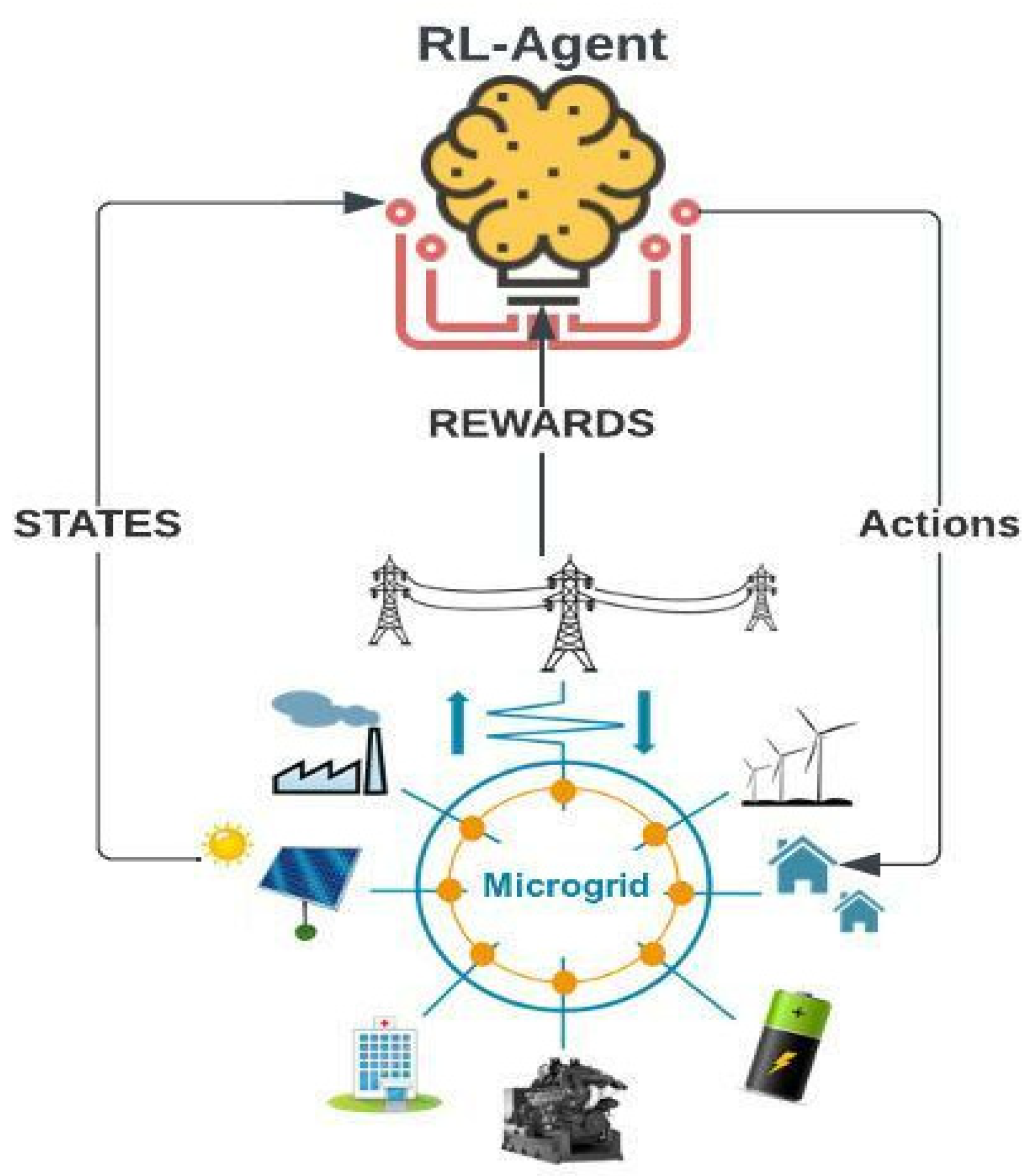
• In this paper, the DRL technique is utilized to handle the time complexity and large dimension space associated with the NP-hardness of optimal charge/discharge scheduling of the BESS. For this purpose, the DRL structure and the state–action–reward tuple are appropriately designed. The continuous deep deterministic policy gradient (DDPG) is used as the training algorithm to avoid the curse of dimensionality issue.
• The DRL can also handle time complexity associated with the nonconvexity of optimization problems for the BESS scheduling and nonlinear power flow. Complementarity constraints should be imposed to avoid simultaneous charge/discharge of the BESS that makes the problem non-convex. Alternatively, using slack integer variables increases the computational burden of the optimization problem.
• Therefore, the trained DRL is practicable for real-time BESS scheduling in MGs for different applications, such as frequency (dynamics) support and ancillary services that are needed to cover intermittent RESs.
• The searching space algorithm is proven to be environment-free and adaptable for EMS in various MG architectures with different scales.
• In order to comprehensively reveal the advantages of this method, the optimization results are compared with the results of the mixed integer nonlinear programming (MINLP) and genetic algorithm (GA).

2. Microgrid Architecture and Modeling

In this paper, we consider the MG including the BESS, a DG under technical constraints, a wind turbine (WT), and a photovoltaic generation (PV) with both deterministic and stochastic power generation, a load with uncertain demand. In order to minimize the 24-h accumulated electricity purchase fee, electricity purchased from the utility grid and hourly electricity prices are also taken into account. The configuration of the MG model is shown in Figure 1.

2.1. PV Generation

In community MGs, photovoltaic power generation equipment is a key renewable energy resource that can transform light energy directly into electrical energy using photovoltaic power production panels. It has a great deal of economic potential and is renowned for its cleanliness and economy. The photovoltaic power generating system, which includes photovoltaic elements including solar panels, AC and DC inverters, solar charge and discharge controllers, and loads, is often positioned on the roof of the building. Grid-connected type, off-grid type, and multi-energy complementing type are the three categories into which solar power-generating devices fall according to the system network structure of the MG. Off-grid photovoltaic power generating systems are appropriate for isolated islands, remote mountainous areas, and other locations, since they cannot interchange electricity with external power networks. A grid-connected photovoltaic power generating system is employed to generate electricity for the community MG under study in this research, which may interchange electrical energy with the main grid or other microgrids.

$$P_{grid}\left(t\right)+P_{pv}\left(t\right)+P_{wt}\left(t\right)=P_{load}\left(t\right)$$

(1)

The output of the photovoltaic power generation system in the MG primarily depends on its power generation, which is inextricably linked to weather factors, such as the highest and lowest temperatures, the average temperature, and the intensity of the day’s light, all of which have an impact on the solar panels’ ability to produce electricity. This paper makes the assumption that the sun shines from 7 am to 8 pm, that its output power varies nonlinearly with light intensity and ambient temperature, and that its light intensity swings from weak to strong and then to weak. The probability density function and mathematical model of a solar power-generating panel are as follows, and the output power of a typical photovoltaic power generation device roughly obeys the distribution:

$$f\left(\frac{I_T}{I_{max}}\right)=\frac{\gamma \left(\alpha +\beta \right)}{\gamma \left(\alpha \right)+\gamma \left(\beta \right)}{\left(\frac{I_T}{I_{max}}\right)}^{\alpha -1}{\left(1-\frac{I_T}{I_{max}}\right)}^{\beta -1}$$

(2)

$$\{\begin{array}{c}\alpha =\mu \left( \mu \left(1-\mu \right)/\sigma ^2-1\right)\\ \beta =\left(1-\mu \right)\left( \mu \left(1-\mu \right)/\sigma ^2-1\right)\end{array}$$

(3)

$$P_{PV}={\phi }_{PV}{S}_{PV}\frac{I_T}{I_S}\left[1+{\alpha }_{PV}\left(T_r-T_s\right)\right]$$

(4)

where γ is the gamma function, and α and β are the relevant parameters of the β distribution. In Formulas (2)–(4), $P_{PV}$ is the rated output power of the photovoltaic power generation system; ${\phi }_{PV}$ is the power frequency reduction coefficient of the photovoltaic power generation system; Tr and Ts represent the actual temperature and standard temperature of the photovoltaic module, respectively; IT is the actual light intensity of the solar panel at 25 °C ambient temperature; and ${\alpha }_{PV}$ is the power temperature coefficient of the PV panel. The value of ${\alpha }_{PV}$ for different materials of the PV panel is not the same, and the general value is ${\alpha }_{PV}$ = −0.45.

2.2. Wind Turbine

Due to its high construction cost, wind power generation equipment, another significant renewable energy resource in MGs, is not as commonly employed as solar power generation equipment. Additionally, as the production of wind energy is very volatile, unpredictable, and is significantly influenced by external variables such as the weather, it is sometimes challenging to make precise short-term projections. Currently, probability distributions are frequently employed to suit the wind speed distribution of wind turbines, with Weibull, Normal, Rayleigh, and other distributions among the most popular choices. The Weibull distribution is one of them and has the following probability density function expression:

$$f\left(v\right)=\frac{k}{a}{\left(\frac{v}{a}\right)}^{k-1}exp\left(-\frac{v^k}{a^k}\right)$$

(5)

$$\{\begin{array}{c}k=\frac{\sigma }{\mu }\\ a=\frac{\mu }{\gamma \left(1+\frac{1}{k}\right)}\end{array}$$

(6)

where the wind turbine’s wind speed $\nu$, its mean value, and its standard deviation are represented by the letters $\sigma$, and $\mu$, respectively. The probability density function of the Welsh distribution, which is currently in widespread usage, can be used to calculate the wind speed distribution of the wind turbine. It is therefore possible to determine the wind turbine’s output power by substituting the wind speed into the mathematical model of the wind turbine. The specific mathematical equation is as follows:

$$P_{WT}=\{\begin{array}{c}\frac{P_e}{v_e-v_{in}}v-\frac{P_e}{v_e-v_{in}}{v}_{in} v_{in}\le v\le v_e\\ P_e v_e\le v\le v_{out}\\ 0 other\end{array}$$

(7)

where $p_{wt}$ is the output power of the wind turbine, Pe is the rated power, ν is the current wind speed, ν_e, ν_in, and ν_out are the rated wind speed, cut-in wind speed, and cut-out wind speed, respectively.

2.3. Battery Energy Storage System (BESS) Modeling

To maintain the stable operation of the MG and balance the system power, an energy storage system must be implemented due to the intermittent and unstable properties of distributed power generating modes, such as solar and wind power. Batteries are frequently employed as high-efficiency energy storage devices, and their internal energy state conforms to the following equation:

$$E_{ESS}\left(t\right)=E_{ESS}\left(t-1\right)+{\eta }_{ch}{P}_{ESS,ch}\left(t\right)\ast \Delta t-\frac{1}{{\eta }_{disch}}{P}_{ESS,disch}\left(t\right)\ast \Delta t$$

(8)

where ${\eta }_{ch}$ and ${\eta }_{disch}$ denote charge and discharge efficiency. The battery’s capacity to charge and discharge at time t is represented by $E_{ESS}\left(t\right)$, while the time t between two charging and discharging operations is represented by $\mathsf{\Delta }t$. The charging and discharging of power $P_{ESS}\left(t\right)$ of the energy storage system in the MG system is typically employed as an essential control variable to take part in the MG energy scheduling, which is the subject of this study. To avoid the charge and discharge happening at the same time, while solving EMS as an optimization problem, we define binary variables.

2.4. Diesel Generator (DG)

The diesel generator (DG) is used to boost its flexibility and independence. When the power production of renewable energy resources becomes stochastic and unreliable, MG relies on electricity stored in the BESS and acquired from the main grid. If the BESS runs out of energy and the main grid has a high electricity price, generating power from DG is the most cost-effective solution to keep loads supplied by MG. The power output and cost factors of DG were modelled as the function of fuel cost:

$$F\left(P_{DG}\left(t\right)\right)=a{P}_{DG}^2\left(t\right)+b{P}_{DG}\left(t\right)+c$$

(9)

where $P_{DG}\left(t\right)$ represents the power output of DG; a, b, and c represent the cost factor of DG.

2.5. Loads and Utility Grid (UG)

In a MG system, the component that uses the most electricity is referred to as the load. The load demand for a fixed MG system is often not customizable since it depends on the MG’s characteristics and the surrounding climate. The load curve is employed as a set quantity of input to the MG system in this paper’s energy scheduling problem. The load is expressed as $P_{load}\left(t\right)$ for time step t.

For the modelling of the utility grid, the power purchased from the grid to MG and the power sold from MG to the grid are mainly considered, representing as $P_{grid}^{+}$ and $P_{grid}^{-}$, respectively. In addition, further descriptions of load and grid will be discussed with the objective function and power balance equation in the next section.

3. DRL-Based MG Energy Management System

3.1. Objective Function

Depending on the requirements of the microgrid system, various control goals can be established, such as minimizing pollutant emissions, cutting back on fuel costs for power generation, reducing voltage offset, cutting back on network active power loss, or increasing voltage stability. Typically, only one control objective or a mix of control objectives can be chosen. This paper seeks to reduce the sum of the cost of power from the external grid and the cost of fuel costs. The form is given in (10):

$$\begin{gathered} \mathrm{F}({\mathit{s}}_{\mathit{t}},{\mathit{a}}_{\mathit{t}},\mathrm{t})=\min [C_{Total}\left(t\right)] \\ {C}_{Total}\left(t\right)={{\displaystyle \int }}_{t=0}^T{C}_{Grid}\left(t\right)\ast P_{Grid}\left(t\right)dt+{{\displaystyle \int }}_{t=0}^{T}F\left(P_{DG} \left(t\right)\right)dt \end{gathered}$$

(10)

where $C_{Grid}, P_{Gird} \mathrm{and} F\left(P_{DG} \left(t\right)\right)$ represent the real-time electricity price, the power generated by the external grid and the fuel cost of DG in time t, respectively, and $P_{grid}, P_{DG}$ satisfies the power balance constraint in (11). $C_{total}$ represents the total cost of the entire MG to obtain electrical energy from the main grid and DG.

$$P_{PV}\left(t\right)+P_{WT}\left(t\right)+P_{ess}\left(t\right)+P_{DG}\left(t\right)+P_{Grid}\left(t\right)=P_{Load}\left(t\right)$$

(11)

Additionally, in this paper, time $t\in D, D=\left\{1,2\dots 24\right\}$ and the unit of t is one hour.

3.2. State Space

The reinforcement learning algorithm DDPG transforms the mentioned control target into a solution form. The energy storage charging and discharging power controller is the agent in the reinforcement learning issue, and the MG mathematical model created in Section 2 serves as the environment. Utilizing the agent and the environment’s ongoing interaction to get the optimal control strategy is the aim of reinforcement learning. As a result, it is necessary to identify the unique representation of the Markov state sequence quadruple (S, A, R, π) for this issue.

For the MG model, the information provided by the environment to the agent is generally renewable energy output, time-of-use electricity price, load, and state of charge of electric energy storage. Therefore, the state space of the microgrid model is defined as:

$${\mathit{s}}_{\mathit{t}}=\left[P_{PV}\left(t\right), P_{WT}\left(t\right),P_{Grid}\left(t\right),P_{Load}\left(t\right),SOC\left(t\right),C_{Grid}\left(t\right)\right]$$

(12)

In the state space: $P_{PV}, P_{WT}$ are the power output of the renewable energy in the t period, kW; $P_{Load}\left(t\right)$ is the load demand of the MG in the t period, kW; $C_{Grid}$ is the time-of-use electricity price (purchased from external grid by microgrid) in the t period (time of use price, TOU), AUD/(kWh); and $SOC\left(t\right)$ is the state of charge of the energy storage system in time t.

3.3. Action Space

After the agent observes the state information of the environment, it selects an action from the action space A according to its own policy set π. Based on controllable devices in MG, the output of DG and the charge/discharge power of the BESS were introduced to the action space. Therefore, the action space of the MG considered in this paper is expressed by:

$${\mathit{a}}_{\mathit{t}}=[P_{ESS}\left(t\right),P_{DG}\left(t\right)]$$

(13)

3.4. System Constraints

To ensure the simulation result is realistic, the energy storage system is set to operate under the constraints of charging and discharging power with a practicable range of the state of charge, and its state of charge also has both limitations to ensure the BESS will not have overheating problems caused by over-voltage or over-current issues. Considering the size and minimum power output of DG, a power constraint is applied by (10):

$$P_{ESS}^{min}\le P_{ESS}\left(t\right)\le P_{ESS}^{max}$$

(14)

$$SO{C}^{min}\le SOC\left(t\right)\le SO{C}^{max}$$

(15)

$$P_{DG}^{min}\le P_{DG}\left(t\right)\le P_{DG}^{max}$$

(16)

3.5. Reward Function

The objective function and the constraints must be combined when creating the reward function R. The following is the definition of the reward function from state t to state $t+1$:

$$R\left({\mathit{s}}_{\mathit{t}},{\mathit{a}}_{\mathit{t}},t\right)=-\left[{{\displaystyle \int }}_t^{t+1}{C}_{grid}\left(t\right)\ast P_{grid}\left(t\right)dt+\beta \left(t\right)\right]$$

(17)

The first component represents the amount of power used, during this time, β(t) = 0, and the second component is the penalty item provided to define the limitations. When the constraints (9)–(11) are not satisfied, β(t) is given a constant with a very big value. When the state–action pair does not exceed the system limitations, the value of β(t) is zero, ensuring the estimation of the agent only depends on the price and power of the utility grid. However, if the state–action pair exceeds the limit, $\beta$(t) is assigned a large penalty value to penalize the taken action by the agent. Reward function maximization is the goal of reinforcement learning; hence a minus sign must be added before these two elements.

4. Deep Reinforcement Learning Algorithm

4.1. DRL Structure

Based on the Markov decision process, reinforcement learning (RL) helps intelligent agents choose actions that will result in the greatest overall reward during their interactions with the environment. An environment and an agent are typically present in RL models, see Figure 2. The agent learns how to react to the environment depending on its current state, while the environment rewards the agent in return. RLs can be categorized as either model-based or model-free, depending on whether explicit environment modeling is necessary. Some typical RL algorithms are as follows: (1) Q-learning, which generates the action for the following step using the quality values Q(s, a) stored in the Q-table, and updates the quality value, where a stands for the learning rate, g for the deduction factor, R for the reward, a and s for the action and state in the current step, and a’ and s’ for the action and state in the following step; (2) the deep Q-network (DQN), which employs deep learning algorithms (such as DNN, CNN, and DT) to produce a continuous Q-quality value in order to get around Q-exponentially learning’s rising computational cost; (3) The policy gradient algorithm, which generates the next-step action based on the policy function (which quantifies the state and action values at the current step) rather than a quality value such as Q; (4) The actor–critic algorithm, which uses the actor to generate the next-step action based on the current-step state and then adjusts its policy based on the score from the critic, whereas the critic uses the critic function to score the actor at the current step [21].

$$\begin{gathered} Q\left(s,a\right)\leftarrow Q\left(s,a\right)+\alpha \left[R+\gamma ma{x}_{a^{\prime }}Q\left(s^{\prime },a^{\prime }\right)-Q\left(s,a\right)\right] \\ s\leftarrow s^{\prime } \end{gathered}$$

(18)

Three types of algorithms may be used to solve reinforcement learning optimization problems: value function-based algorithms, policy gradient-based algorithms, and search-based and supervised algorithms [24]. The solution techniques based on the value function are the main topic of this work. Examples include the dynamic programming algorithm, the Monte Carlo algorithm, the time series difference algorithm, etc. Among these, the dynamic programming approach is useful for addressing problems when there is a model, and the state space has a small dimension. The downside of the Monte Carlo approach is that it requires entire state sequence information, which is challenging to get in many aperiodic systems. It is a straightforward algorithm that is not model-based. A complete state sequence is not necessary for the time series difference approach to estimate the value function. The online difference algorithm SARSA and the offline difference algorithm Q-learning algorithm are two examples of the traditional time series difference approach. Both approaches retain a Q-table to tackle minor issues. The problem with reinforcement learning is when the state and action space is continuous or discrete on a very large scale, it is necessary to keep an exceptionally big Q-table, which poses storage challenges. However, this issue was resolved by the advancement of deep neural networks. A deep reinforcement learning technique that is more suited for difficult issues may be produced by using deep neural networks rather than Q-tables. Deep Q-learning (deep Q-network, DQN) is a common algorithm.

$$Q\left(\mathit{s},\mathit{a}\right)\leftarrow Q\left(\mathit{s},\mathit{a}\right)+\alpha \delta$$

(19)

The action value function is represented by $Q\left(\mathit{s},\mathit{a}\right)$, while the learning rate is represented by $\delta$. The ideal reinforcement learning control method can be discovered when the update formula converges. The DQN replaces the Q-function $Q\left(\mathit{s},\mathit{a}/\mathit{Z}\right)$ in Q-learning by using a deep neural network. Following the calculation of the current target Q-value using Formula (3), the neural network’s parameter is adjusted based on the mean square error between the current target Q-value and the Q-value provided by the Q-network.

4.2. Deep Deterministic Policy Gradient (DDPG)

Based on the DRL algorithm that was introduced above, DDPG is adopted as the optimization algorithm to reduce the MG’s cost. DDPG is an RL algorithm that learns the policy and Q-function simultaneously. This approach processes off-policy data through the Bellman equation to achieve the learning goals towards the Q-function, and DDPG then learns the policy from the Q-function. According to the Q-function: ${\mathcal{Q}}^{\ast }\left(\mathit{s},\mathit{a}\right)$ and current state space, the optimized action ${\mathit{a}}^{\ast }\left(\mathit{s}\right)$ can be obtained from this equation:

$${\mathit{a}}^{\ast }\left(\mathit{s}\right)=\mathbf{arg}\underset{\mathit{a}}{\mathbf{max}}{\mathcal{Q}}^{\ast }\left(\mathit{s},\mathit{a}\right)$$

(20)

The loss function of the Q-network can be described as the learning process of the Q-network under the guidance of the reward function. By using the temporal difference principle, the loss function can be defined as (16):

$$\mathit{𝓛}\left({\mathit{𝔀}}^{\mathit{C}}\right)={\left[\mathcal{Q}\left(\mathit{s},\mathit{a}|{\mathit{𝔀}}^{\mathit{Q}}\right)-\left(\mathit{r}+\mathit{\gamma }\left(\mathcal{Q}\left(\mathit{s}\_,\mathit{a}\_|{\mathit{𝔀}}^{\mathit{Q}}\right)\right)\right)\right]}^2$$

(21)

In this formula, $\mathcal{Q}\left(\mathit{s},\mathit{a}|{\mathit{𝔀}}^{\mathit{Q}}\right)$ represents the Q-function in the current states and the accumulated future reward of the agent when the action of this state was executed. For the next states, s_, the Q-function is defined as the same as the last states. In $\mathcal{Q}\left(\mathit{s}\_,\mathit{a}\_|{\mathit{𝔀}}^{\mathit{Q}}\right)$, s_ and a_ represent the state–action pair in the next states and ${\mathit{𝔀}}^{\mathit{Q}}$ is the weight of the Q-network. The actions in DDPG are determined by the policy; r represents the reward corresponding to the excused action from the current states s to the next states s_.

The objective function for the Q-network is defined as:

$$\mathit{F}\left({\mathit{𝔀}}^{\mathit{C}}\right)=min\left[\mathit{𝓛}\left({\mathit{𝔀}}^{\mathit{C}}\right)\right]$$

(22)

By introducing the learning rate $\mathit{\theta }$, the update date mode can be described as:

$${\mathit{𝔀}}^{\mathit{C}}⟵{\mathit{𝔀}}^{\mathit{C}}+\mathit{\theta }{\mathbf{\nabla }}_{{\mathit{𝔀}}^{\mathit{C}}}\mathit{𝓛}\left({\mathit{𝔀}}^{\mathit{C}}\right)$$

(23)

The DDPG is presented in Algorithm 1.

Algorithm 1 Deep deterministic policy gradient
1:	Input: Initialize Q-function and policy, clean out replay buffer $\mathcal{D}$;
2:	Define objective parameters for Q-function and policy in $\theta$ and $\varphi$;
3:	Loop;
4:		Based on current observation, generate state-action pair $\left(\mathit{s},\mathit{a}\right)$;
5:		Practice action in the environment;
6:		Obtain the reward $\mathit{r}$ and move to next state ${\mathit{s}}^{\prime }$, check the ending signal $\mathit{e}$;
7:		$\mathrm{Append}(\mathit{s},\mathit{a}, \mathit{r},{\mathit{s}}^{\prime },\mathit{e})$ to relay buffer $\mathcal{D}$;
8:		$if$s’ is the last state and ending signal $\mathit{e}$ is true;
9:			$for$ training episodes do;
10:				$\mathrm{Import}\mathrm{transients}\mathcal{T}\left(\mathit{s},\mathit{a}, \mathit{r},{\mathit{s}}^{\prime },\mathit{e}\right)$ from $\mathcal{D}$;
11:				Solve the objectives by transients   $O\left(\mathit{r},{\mathit{s}}^{\prime },\mathit{d}\right)=r+\gamma \left(1-e\right)Q_{obj}\left[s^{\prime },P_{obj}\left(s^{\prime }\right)\right]$;
12:				Obtain updated Q-function   $\mathbf{\nabla }\frac{1}{\left|\mathcal{T}\right|}{{\displaystyle \sum }}_{\left(\mathit{s},\mathit{a}, \mathit{r},{\mathit{s}}^{\prime },\mathit{e}\right) \in \mathcal{T}}{\left(Q\left(\mathit{s},\mathit{a}\right)-O\left(\mathit{r},{\mathit{s}}^{\prime },\mathit{d}\right)\right)}^2$;
13:				Obtain updated policy   $\mathbf{\nabla }\frac{1}{\left|\mathcal{T}\right|}{\displaystyle \sum }_{\mathit{s} \in \mathcal{T}}{Q}_{obj}\left(s^{\prime },P_{obj}\left(s^{\prime }\right)\right)$;
14:				Update objective networks’ weight   ${\mathit{𝔀}}^{\mathit{C}}⟵{\mathit{𝔀}}^{\mathit{C}}+\mathit{\theta }{\mathbf{\nabla }}_{{\mathit{𝔀}}^{\mathit{C}}}\mathit{𝓛}\left({\mathit{𝔀}}^{\mathit{C}}\right)$;
15:				end for;
16:			end if;
17:		until reward convergence.

5. Case Study

5.1. Simulation Settings

Table 1. Purchases and sell price.

Electricity Purchase (AUD/kWh)	Electricity Sells (AUD/kWh)
1.1	0.85

demonstrates the trading price between the utility grid and MG.

Table 2. Input parameters.

PV (kW)	WT (kW)	Load (kWh)	Price (AUD/kWh)
0	50	50	0.434137
0	50	60	0.42391
0	50	60	0.42
0	50	54	0.426393
0	40	40	0.448192
10	30	40	0.503548
25	30	65	0.598517
30	40	79	0.63099
50	45	100	0.650717
60	45	120	0.654483
65	50	110	0.661257
75	45	77	0.645917
75	45	70	0.626667
70	55	68	0.633886
70	55	75	0.639901
60	60	90	0.647722
40	65	117	0.667376
27	60	125	0.683024
10	55	130	0.7
0	55	125	0.673981
0	60	130	0.623744
0	60	90	0.558902
0	55	80	0.493186
0	55	75	0.456695

and Figure 3 present system parameters, including the power generation of PV and WT, the load demand, and the electricity price from the utility grid side. Each column has 24 rows, and each row indicates the corresponding parameter in one hour, which means the sampling period time is one hour and the whole period of simulation is 24 h. The parameters in Table 2 are highly determined by realistic weather and load demand. This case study considers a deterministic scenario on a sunny day. PV output reaches a peak in the afternoon and WT randomly generates electricity fluctuating around its average value. Load demand has two peaks during both daytime and night. Market price increases when load demand is high. Otherwise, electricity sells in a cheap way when a demand valley is shown. Through this simplified MATLAB simulation model, the effectiveness of the DDPG algorithm is demonstrated. The program of the model made use of the Reinforcement Learning Toolbox in MATLAB to train the Q-agent and policy. In addition, to make comparisons of simulation results, YALMIP/GUROBI, which is a commercial optimization solver, is practiced for processing the nonlinear programming model. Here, we further explain the profits and optimality of the proposed algorithms.

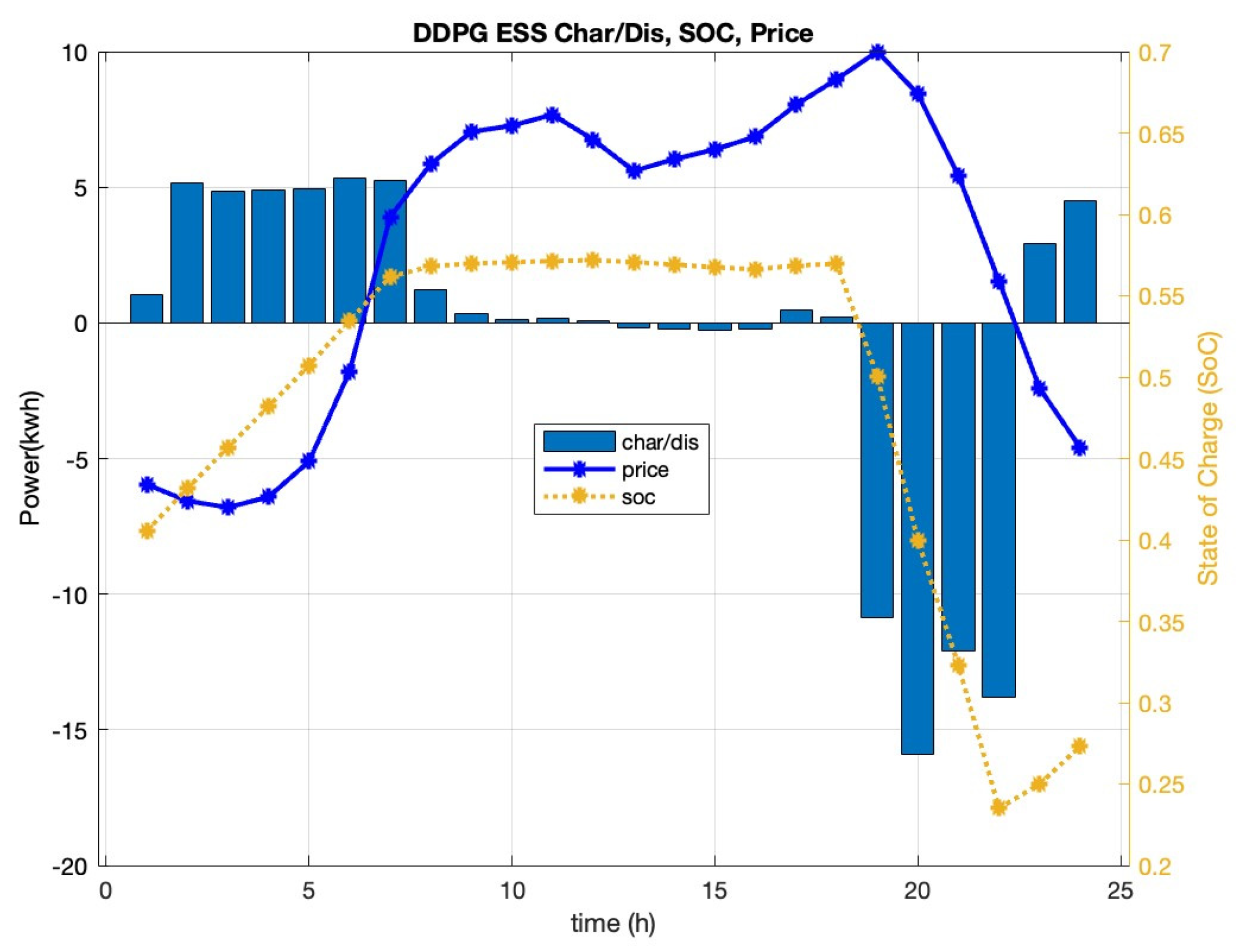
5.2. Simulation Results and Discussion

From the beginning, Figure 4 demonstrates the curve of the reward function. The graph shows that after around 550 episodes of training, the agent’s reward infinitely approaches zero. As a consequence, the agents are effectively trained, and the simulation results are effective. Part of the code can be shown in Algorithm 1.

Having illustrated the realism and validity of the simulation, Figure 5 shows the power output profiles of ESS, DG, load, and utility grid. The load profile shows that, during the daytime, electricity demand keeps rising from 6 to 10 am, resulting in the first peak value at 125 kW. Then, demand descends to 75 kW at 1 pm, before it quickly lifts to the second peak value, which is 130 kW at 7 pm. The peak value remains for 2 h and demand decreases to 70 kW at the end of the day. Regarding the power exchange between the MG and the utility grid, most of the time, MG sells electricity to the utility grid and purchases electricity from the utility grid when the load demand increases to the second peak value during the evening. DG power output rises from midnight for 1 h to 40 kW and slowly drops to 30 kW in 17 h. DG profile then directly drops to zero in one hour and returns to 30 kW at 11 pm.

Figure 6 demonstrates the SOC profile of ESS. Considering the SOC profile with the BESS charge and discharge profile, the state of charge starts from 40% and charges to approximately 60% in 0–6 am. Then the BESS module turns to float charging mode, keeping the SOC at 60% until the second load peak comes. From about 18 pm, a dramatic decreasing trend is found. The BESS discharges and supplies the load with the utility grid and RES from 18 pm to 23 pm. Finally, the BESS is slightly charged from RES and grid for 1 h.

In order to describe the effectiveness of the DDPG algorithm, the charge/discharge profile of ESS, state of charge, and electricity price are plotted on one graph. As shown in Figure 7, the BESS charges when the electricity price is relatively low, resulting in a rise in SOC. On the other hand, the BESS discharges when the price is relatively high, resulting in a decrease in SOC. Such a kind of energy management schedule strategy produced by DDPG lowers the cost of power procurement while increasing the profitability of power sales. Figure 8 demonstrates the cost profile in MG. The system only has 5 h at a high cost. It remains at a low cost for 14 h and has a negative cost, i.e., profit for 5 h. Therefore, the MG with DDPG scheduled EMS can effectively reduce the operating cost.

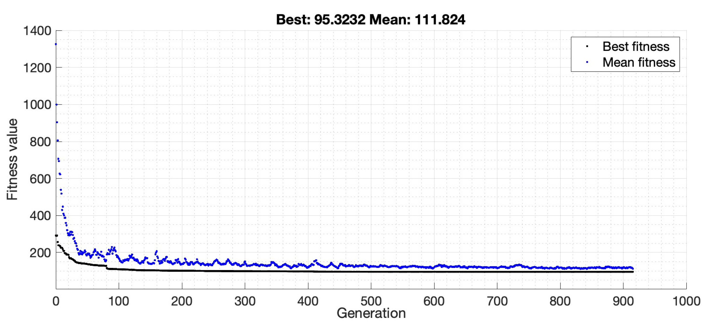
5.3. Results Comparision and Analysis

To demonstrate the efficacy of DDPG further, we compared its performance with the GA and the MINLP method, with identical simulation data. MINLP is an adaptable modeling tool for EMS because it can address nonlinear problems with continuous and integer variables. Figure 9 shows the convergence process of the genetic algorithm, illustrating its effectiveness.

Table 3. DG cost parameters.

a	b	c
0.001	0.15	77.44

shows the cost parameters of DG, corresponding to Formula (9).

The following three figures demonstrate the difference between DDPG, MINLP, and GA in electricity trading between MG and the utility grid. According to Figure 10a, from 0 am to 17 pm, DDPG has an outstanding performance that sells electricity from MG to the utility grid the whole time, and for the rest of the period, DDPG purchases electricity at an average of 40 kW per hour. Figure 10b shows that MINLP spends half of the whole time period selling electricity from MG to the grid, and the total amount of sold electricity is around 300 kWh, which is the half amount of DDPG. Considering the purchased electricity, MINLP purchased almost the same amount of electricity from the grid as the amount it sells. Figure 10c reveals that from 0 am to 17 pm, GA has two hours for purchase with a lower average power output value than DDPG. Hence, we can conclude that DDPG has the extraordinary capability of selling energy from MG to the utility grid.

In addition, focusing on the energy storage system, the following six figures demonstrate the BESS performance including charge and discharge power and state of charge, obtained by three introduced algorithms. Table 2 and

Table 4. System Constraints.

${\mathbf{P}}_{\mathbf{E}\mathbf{S}\mathbf{S}}\left(\mathbf{k}\mathbf{W}\right)$	${\mathbf{P}}_{\mathbf{D}\mathbf{G}}\left(\mathbf{k}\mathbf{W}\right)$	$\mathbf{S}\mathbf{O}\mathbf{C}$
$\left[-40, 40\right]$	$\left[0, 60\right]$	$\left[0.2, 0.85\right]$

present the system constraints, such as the charge and discharge power constraints of the energy storage system, the power output constraints of DG, and the constraints of ESS’s state of charge.

Based on Figure 11, it is obvious that DDPG stores energy in the BESS when the utility power price is lower in a day, and DDPG discharges ESSs from 6 pm to 10 pm, selling electricity to the grid at the peak value of the price, earning the maximum profit for MG during this period. It is worth noting that the cost of DG was set to 0.5 AUD/kWh, and Figure 3 shows that the electricity price is higher than 0.5 in the period of 6 am to 23 pm. From that perspective, theoretically, DG should remain at its maximum output when its cost is lower than the electricity price, as the results are shown in Figure 11, for the linear programming DG output profile. On the other hand, the BESS should be charged as fully as possible (under the system constraints), which is the most desirable energy management schedule. However, DDPG just slightly charges the BESS for 20% and stops the charging/discharging movement until the second price peak is reached. Additionally, according to Figure 12, we notice that GA has a better performance on both the BESS and DG power profiles. The curve is greatly shaking due to the prediction error, but the charging and discharging depth of the BESS and power output of DG is greater than the corresponding value of DDPG.

However, with the unsatisfied profile produced by DDPG, it can be a kind of advantage that the BESS and DG do not reach their constraints, which results in less degradation cost for long-term operation in MG and reduces the possibility for the happening of safety issues.

Table 5. Result comparisons.

	DDPG-Based DRL	MINLP	GA
Purchasing Cost (AUD)	87.333	45.772	88.406
Computation Time (s)	1.202061	2.745373	23.328163

compares the simulation results of three different techniques. In terms of the overall cost created by EMS, MINLP has the lowest purchasing cost, with a cost of 45.772 AUD per day. GA comes in second, followed by DDPG. However, in terms of computation time, DRL can be processed faster than GA and MINLP.

Compared with MINLP and GA, in this small scale and accurately modeled MG, DDPG’s exploring strength is not as strong in finding a policy with high accuracy as MINLP, because during the space searching process, agent actions are effect by system noise. However, if we consider the DDPG in a more realistic scenario, DDPG does have its unique advantages. For example, MINLP can only be implemented on a small-scale MG system, as the large-scale MG with hierarchy architecture will make the mathematical modeling process extremely complex and computationally time-consuming, which is not practical in the real world. In contrast, as DRL is a set of model-free algorithms, DDPG can adapt to any unknown MG structure. Additionally, compared with the GA, DDPG can be quickly used for a new dataset that only spends a very short time for secondary training for its deep neural network. The other two algorithms take a long time for modeling and convergence, respectively. Lastly, DDPG has the capability to handle the task of a high degree of stochastic data, which is very common in RES-based MG. The other two are not compatible due to the same reason. These three unique characteristics of DDPG determine that it is valuable and realistic to reduce the purchasing cost of MG.

6. Conclusions

This paper developed a DRL-based MG energy management system and obtained an energy schedule policy for one day with a sampling time of one hour. EMS policy aimed to reduce the MG electricity cost. The structure of the DRL agent was designed by defining appropriate functions related to the state–action–reward tuple. The DDPG algorithm was adopted to train the DRL agent using a simulated MG. The performance of the DRL agent was compared with the results of the MINLP and GA. This paper revealed both the advantages and disadvantages of the DDPG-based DRL.

The DDPG-based DRL agent for EMS in MGs has the following strengths and drawbacks:

• The DRL agent tries a large number of trial-and-error episodes during training, by which all possible combinations of the BESS charge/discharge schedule, with various initial SoC, are tested. The DDPG optimizes the DRL network to maximize the rewards and thus minimizes the purchasing cost. This training process costs computational costs.
• In an MG with a simple structure and determinant load/weather, the DRL agent would cost more computation time for training compared with GA and MINLP. In the simulated scenario, the DRL achieved higher purchasing costs, but smaller computation time for real-time action.
• The training process of DRL would increase in a large-scale MG system, but after training, the DRL agent reveals superior computation for real-time performance.
• The DRL agent is able to deal with uncertainties that happened in MG, such as stochastic power generation produced by RESs in MG.
• When the EMS is adapted to a new location, e.g., replacing a new database with EMS, the DRL agent can quickly be adapted by training its deep neural network.

In future development, with the aid using the transfer learning principle, GA and MINLP can be used for training the DRL for enhancing its rewards to approach linear programming results.

References

1. Olivares, D.E.; Mehrizi-Sani, A.; Etemadi, A.H.; Cañizares, C.A.; Iravani, R.; Kazerani, M.; Hajimiragha, A.H.; Gomis-Bellmunt, O.; Saeedifard, M.; Palma-Behnke, R.; et al. Trends in microgrid control. IEEE Trans. Smart Grid 2014, 5, 1905–1919. [Google Scholar] [CrossRef]
2. Moradi, M.H.; Eskandari, M.; Hosseinian, S. Operational Strategy Optimization in an Optimal Sized Smart Microgrid. IEEE Trans. Smart Grid 2015, 6, 1087–1095. [Google Scholar] [CrossRef]
3. Tabar, V.S.; Jirdehi, M.A.; Hemmati, R. Energy management in microgrid based on the multi objective stochastic programming incorporating portable renewable energy resource as demand response option. Energy 2017, 118, 827–839. [Google Scholar] [CrossRef]
4. Asadi, Y.; Eskandari, M.; Mansouri, M.; Savkin, A.V.; Pathan, E. Frequency and Voltage Control Techniques through Inverter-Interfaced Distributed Energy Resources in Microgrids: A Review. Energies 2022, 15, 8580. [Google Scholar] [CrossRef]
5. Shi, W.; Li, N.; Chu, C.C.; Gadh, R. Real-time energy management in microgrids. IEEE Trans. Smart Grid 2015, 8, 228–238. [Google Scholar] [CrossRef]
6. Eskandari, M.; Li, L.; Moradi, M.H.; Siano, P.; Blaabjerg, F. Optimal voltage regulator for inverter interfaced distributed generation units part I: Control system. IEEE Trans. Sustain. Energy 2020, 11, 2813–2824. [Google Scholar] [CrossRef]
7. Eskandari, M.; Savkin, A.V. A Critical Aspect of Dynamic Stability in Autonomous Microgrids: Interaction of Droop Controllers through the Power Network. IEEE Trans. Ind. Inform. 2021, 18, 3159–3170. [Google Scholar] [CrossRef]
8. Eskandari, M.; Savkin, A.V. On the Impact of Fault Ride-Through on Transient Stability of Autonomous Microgrids: Nonlinear Analysis and Solution. IEEE Transactions on Smart Grid 2021, 12, 999–1010. [Google Scholar] [CrossRef]
9. Uzair, M.; Eskandari, M.; Li, L.; Zhu, J. Machine Learning Based Protection Scheme for Low Voltage AC Microgrids. Energies 2022, 15, 9397. [Google Scholar] [CrossRef]
10. Zhou, N.; Liu, N.; Zhang, J.; Lei, J. Multi-objective optimal sizing for battery storage of PV-based microgrid with demand response. Energies 2016, 9, 591. [Google Scholar] [CrossRef]
11. Mansouri, M.; Eskandari, M.; Asadi, Y.; Siano, P.; Alhelou, H.H. Pre-Perturbation Operational Strategy Scheduling in Microgrids by Two-Stage Adjustable Robust Optimization. IEEE Access 2022, 10, 74655–74670. [Google Scholar] [CrossRef]
12. Rezaeimozafar, M.; Eskandari, M.; Amini, M.H.; Moradi, M.H.; Siano, P. A Bi-Layer Multi-Objective Techno-Economical Optimization Model for Optimal Integration of Distributed Energy Resources into Smart/Micro Grids. Energies 2020, 13, 1706. [Google Scholar] [CrossRef] [Green Version]
13. Eskandari, M.; Rajabi, A.; Savkin, A.V.; Moradi, M.H.; Dong, Z.Y. Battery energy storage systems (BESSs) and the economy-dynamics of microgrids: Review, analysis, and classification for standardization of BESSs applications. J. Energy Storage 2022, 55, 105627. [Google Scholar] [CrossRef]
14. Zheng, C.; Eskandari, M.; Li, M.; Sun, Z. GA-Reinforced Deep Neural Network for Net Electric Load Forecasting in Microgrids with Renewable Energy Resources for Scheduling Battery Energy Storage Systems. Algorithms 2022, 15, 338. [Google Scholar] [CrossRef]
15. Nguyen, T.T.; Nguyen, N.D.; Nahavandi, S. Deep reinforcement learning for multiagent systems: A review of challenges, solutions, and applications. IEEE Trans. Cybern. 2020, 50, 3826–3839. [Google Scholar] [CrossRef] [PubMed] [Green Version]
16. Mousavi, S.S.; Schukat, M.; Howley, E. Deep reinforcement learning: An overview. In Proceedings of the SAI Intelligent Systems Conference, London, UK, 7–8 September 2017; pp. 426–440. [Google Scholar]
17. Hua, H.; Qin, Y.; Hao, C.; Cao, J. Optimal energy management strategies for energy Internet via deep reinforcement learning approach. Appl. Energy 2019, 239, 598–609. [Google Scholar] [CrossRef]
18. Khooban, M.H.; Gheisarnejad, M. A novel deep reinforcement learning controller-based type-II fuzzy system: Frequency regulation in microgrids. IEEE Trans. Emerg. Top. Comput. Intell. 2020, 5, 689–699. [Google Scholar] [CrossRef]
19. François-Lavet, V.; Taralla, D.; Ernst, D.; Fonteneau, R. Deep reinforcement learning solutions for energy microgrids management. In Proceedings of the European Workshop on Reinforcement Learning (EWRL 2016), Barcelona, Spain, 3–4 December 2016. [Google Scholar]
20. Du, Y.; Zandi, H.; Kotevska, O.; Kurte, K.; Munk, J.; Amasyali, K.; Mckee, E.; Li, F. Intelligent multi-zone residential HVAC control strategy based on deep reinforcement learning. Appl. Energy 2021, 281, 116117. [Google Scholar] [CrossRef]
21. Jin, X.; Lin, F.; Wang, Y. Research on Energy Management of Microgrid in Power Supply System Using Deep Reinforcement Learning. In IOP Conference Series: Earth and Environmental Science; IOP Publishing: Bristol, UK, July 2021; Volume 804, Number 3. [Google Scholar]
22. Yoldas, Y.; Goren, S.; Onen, A. Optimal Control of Microgrids with Multi-stage Mixed-integer Nonlinear Programming Guided Q-learning Algorithm. J. Mod. Power Syst. Clean Energy 2020, 8, 1151–1159. [Google Scholar] [CrossRef]
23. Phan, B.C.; Lai, Y.C. Control strategy of a hybrid renewable energy system based on reinforcement learning approach for an isolated microgrid. Appl. Sci. 2019, 9, 4001. [Google Scholar] [CrossRef]
24. Zeng, P.; Li, H.; He, H.; Li, S. Dynamic energy management of a microgrid using approximate dynamic programming and deep recurrent neural network learning. IEEE Trans. Smart Grid 2018, 10, 4435–4445. [Google Scholar] [CrossRef] [Green Version]
25. Li, J.; Chen, S.; Wang, X.; Pu, T. Research on load shedding control strategy in power grid emergency state based on deep reinforcement learning. CSEE J. Power Energy Syst. 2022, 8, 1175. [Google Scholar]
26. Antonopoulos, I.; Robu, V.; Couraud, B.; Kirli, D.; Norbu, S.; Kiprakis, A.; Flynn, D.; Elizondo-Gonzalez, S.; Wattam, S. Artificial intelligence and machine learning approaches to energy demand-side response: A systematic review. Renew. Sustain. Energy Rev. 2020, 30, 109899. [Google Scholar] [CrossRef]
27. Kumari, A.; Tanwar, S. A reinforcement-learning-based secure demand response scheme for smart grid system. IEEE Internet Things J. 2021, 9, 2180–2191. [Google Scholar] [CrossRef]
28. Lei, L.; Tan, Y.; Dahlenburg, G.; Xiang, W.; Zheng, K. Dynamic energy dispatch based on deep reinforcement learning in IoT-driven smart isolated microgrids. IEEE Internet Things J. 2020, 8, 7938–7953. [Google Scholar] [CrossRef]
29. Huang, Y.; Li, G.; Chen, C.; Bian, Y.; Qian, T.; Bie, Z. Resilient distribution networks by microgrid formation using deep reinforcement learning. IEEE Trans. Smart Grid 2022, 13, 4918–4930. [Google Scholar] [CrossRef]
30. Zhao, J.; Li, F.; Mukherjee, S.; Sticht, C. Deep Reinforcement Learning based Model-free On-line Dynamic Multi-Microgrid Formation to Enhance Resilience. IEEE Trans. Smart Grid 2022. [Google Scholar] [CrossRef]
31. Garcia-Torres, F.; Bordons, C.; Ridao, M.A. Optimal Economic Schedule for a Network of Microgrids With Hybrid Energy Storage System Using Distributed Model Predictive Control. IEEE Trans. Ind. Electron 2019, 66, 1919–1929. [Google Scholar] [CrossRef]
32. Wei, Q.; Liu, D.; Shi, G. A novel dual iterative Q-learning method for optimal battery management in smart residential environments. IEEE Trans. Ind. Electron 2015, 62, 2509–2518. [Google Scholar] [CrossRef]
33. Du, Y.; Li, F. Intelligent multi-microgrid energy management based on deep neural network and model-free reinforcement learning. IEEE Trans. Smart Grid 2019, 11, 1066–1076. [Google Scholar] [CrossRef]
34. Rana, M.J.; Zaman, F.; Ray, T.; Sarker, R. Real-time scheduling of community microgrid. J. Clean. Prod. 2021, 286, 125419. [Google Scholar] [CrossRef]
35. Mocanu, E.; Mocanu, D.C.; Nguyen, P.H.; Liotta, A.; Webber, M.E.; Gibescu, M.; Slootweg, J.G. On-line building energy optimization using deep reinforcement learning. IEEE Trans. Smart Grid 2018, 10, 3698–3708. [Google Scholar] [CrossRef]
Figure 1. Microgrid architecture, which consists of DERs including RESs (PV and WT), DG, and the battery ESS, and loads. The MG can be disconnected from the utility grid and work in autonomous mode, where DERs supply the local load and the BESS holds the consumption–production balance.
Energies 16 00090 g001
Figure 2. Schematic diagram of RL.
Energies 16 00090 g002
Figure 3. Profiles of input parameters.
Energies 16 00090 g003
Figure 4. Training profile.
Energies 16 00090 g004
Figure 5. Power profile of DDPG, grid, BESS, and load.
Energies 16 00090 g005
Figure 6. BESS SOC state of charge.
Energies 16 00090 g006
Figure 7. BESS power, SOC, and price profile.
Energies 16 00090 g007
Figure 8. MG cost profile.
Energies 16 00090 g008
Figure 9. GA convergence process.
Energies 16 00090 g009
Figure 10. Performance comparison for grid power profile: (a) DDPG; (b) MINLP; and (c) GA grid.
Energies 16 00090 g010
Figure 11. Performance comparison for the BESS and DG output profile: (a) DPPG; (b) MINLP; and (c) GA.
Energies 16 00090 g011
Figure 12. Performance comparison for SOC Profile: (a) DDPG; (b) MINLP; and (c) GA.
Energies 16 00090 g012