Abstract
Ice slurry is a high energy density coolant with excellent flow, phase change, and thermophysical properties. In order to investigate the recovery of ice slurry flowing through a local large heat flux segment, a 3D Eulerian-Eulerian model based on the granular kinetic theory considering the flow and melting phase change of ice slurry is developed. Sensitivity analysis of interphase forces is carried out. A comparison of the pressure drop, solid phase velocity, and heat transfer coefficient with empirical data is carried out, respectively. The calculated results are in good agreement with the experimental results, indicating that the numerical model could accurately describe the flow and melting characteristics. Thermophysical field distributions, the axial variation of ice volume fraction (IVF), recovery curve, the average heat transfer coefficient, as well as the re-uniformization length are obtained. After passing through local large heat flux segment, due to shear stress action, the IVF and the particle uniformity of the cross section have recovery characteristics. The gradient of the recovery curve decreases with increasing inlet IVF as well as with increasing Reynolds number. After the local large heat flux increases to a certain value, its effect on the recovery curve of the ice slurry is small. The re-uniformization length increases as the local large heat flux increases. The average heat transfer coefficient of local large heat flux segment increases due to damage of the boundary layer. These results can provide a theoretical basis for the design of ice slurry systems in practical application.
1. Introduction
Ice slurry, which is an appealing phase change cold storage material, consists of a mixture of carrier liquid and ice particles (which usually has a diameter of 0.1–1 mm) [1,2,3]. The solid and liquid two phase flow characteristics of ice slurry endow it with good fluidity, thermal, and transport properties. The substantial latent heat ice slurry (334 kJ/kg) [4] can effectively reduce the amount of pipe used in transit, lower the energy consumption of pumping, and reduce the size of the heat exchanger. It is used as both cold storage medium and heat exchange medium in various fields, being widely studied in recent years and presents a broad application prospect [5,6,7,8].
Ma et al. [9] provided a comprehensive review of the thermal fluid properties of different shell-less phase change slurry PCS from various aspects. Wang et al. [6,10,11] reviewed the characteristics of flow and heat transfer for ice slurry in cooling systems and studied the fluidity characteristic of ice slurry in horizontal, vertical, and 90° elbow pipes, respectively. It is easy to see that the characteristics of the ice slurry (additive concentration, additive type) as well as the structure of the flowing pipe and different thermal boundary conditions have a large influence on the heat transfer and flow characteristics of the ice slurry.
Flow and heat transfer experiments on ice slurry are commonly performed with round tubes, and scholars have conducted a series of experiments with different ice slurry. Grozdek et al. [12,13] used the 10.3% aqueous solution of ethanol while Lee et al. [14] experimentally studied the 6.5% ethanol-water solution ice slurry. Niezgoda-Zelasko [15,16] developed dimensionless relations based on experimental results to estimate local heat transfer coefficient values for different conditions. Kumano et al. [17] investigated the effect of ice slurry additive mass concentration on heat transfer and found that the effect was not significant. In addition to ice slurry transport in flat pipes, scholars have also conducted experimental studies on specially shaped pipes and heat exchanger coils. Mi et al. [18] conducted many experiments to study the performance of ice slurry flow through a plate heat exchanger with different mass concentrations. Ohira et al. [19] studied the effect of different shapes of pipes on pressure as well as heat transfer. The study of solid-liquid two-phase slurry is not limited to ice slurry. Experimental studies have also been conducted on cryogenic slurry. Li et al. [20] investigated experimentally and numerically the heat transfer characteristics of slush nitrogen and obtained a modified empirical correlation equation for the Nusselt number.
Researchers have also developed numerical models to simulate and analyze the flow characteristics of ice slurry, and the more commonly used model is the Euler-Euler model. Hu et al. [21] performed isothermal flow simulations of ice pigging using the Euler-Euler model. The numerical results indicated an uneven shear stress distribution along the flow. Gao et al. [22] employed an Euler-Euler approach considering interphase transfer mechanisms. It was found that the ice particle distribution as well as homogeneity is related to the velocity and the ice content. Cai et al. [23] conducted a numerical study on the heat transfer enhancement of ice slurry in horizontal pipes and found that pulsating flow can largely improve the heat transfer characteristics of ice slurry. Yadav et al. [24] investigated ice slurry flow in elliptical pipes under isothermal and non-isothermal conditions. The results showed that the melting of ice slurry in elliptical tubes was inhibited compared to that in circular pipes. Xu et al. [25] numerically simulated the flow of ice slurry in the inlet straight pipe of shell-and-tube heat exchanger. It was shown that the appearance of turbulence in the outlet cross-section and the degree of ice slurry stratification were related to the inlet velocity. Jin et al. [26,27] numerically investigated the flow characteristics of slush nitrogen. It was seen in some published experimental work that the pressure drop of slush nitrogen is larger than that of subcooled liquid nitrogen. Shi et al. [28,29] numerically investigated the characteristics of heat transfer of hydrate slurry in horizontal 90° bends and U-pipe.
It was found that the curved section leads to the appearance of secondary flows, vortices, and boundary layer separation. Simulation studies have also been performed using other numerical modeling methods, such as VOF models, single-fluid models, Boltzmann method, and other complex models. Li et al. [30] used VOF model to numerically study the heat transfer characteristics of ice slurry. Onokoko et al. [31] developed a 3D single phase model to study isothermal ice slurry flow in laminar and turbulent conditions. Onokoko et al. [32,33] proposed a simpler model for studying CFD models of isothermal ice slurry flow. Suzuki et al. [34] used the thermal immersed boundary–lattice Boltzmann method to simulate the interactions between particles and liquid in ice slurry flow as well as to study the Nusselt number correlation equation. Bordet et al. [35,36] used a model that captured more complex flow characteristics, particularly near-wall boundary layers and secondary flow, to study the ice slurry dynamical behavior. Languri et al. [37] quantified and discussed the heat transfer data of MPCM additives with different mass fractions in the base solution in detail, and obtained flow rate and heat transfer curve relationships.
The above is presented in an experimental study as well as a numerical study. The experimental part is classified by pipe structure into circular pipes as well as other complex pipes. The next part focuses on the numerical simulation studies, which are mainly introduced by numerical method classification, focusing on the studies conducted using the Euler-Euler model, enumerating the simulation studies, such as the VOF method and the single fluid method. A general review of the study of heat transfer characteristics of ice slurry is presented. However, there are few studies on the characteristics of flow-melt and recovery for ice slurry in the transportation pipe with local large heat flux segment, e.g., flowing through pumps, heat exchangers, heating elements, etc.
In the present paper, to further investigate the flow and melting characteristics of ice slurry as it flows through the pipe with local large heat flux segment, a 3D numerical model based on granular kinetic theory and considering flow and melting is proposed in Section 2. The numerical model developed is validated against the experimental data in Section 3. In Section 4, the results are given and discussed. The effects of various parameters on the thermophysical field distribution, axial IVF variation, average heat transfer coefficient, and the re-uniformization length are investigated in particular. The conclusion is provided eventually in Section 5.
2. Mathematical Model and Numerical Implementation
2.1. Physical Model
As ice slurry flows through the pipeline system, it may pass through pumps, flanges, heat exchanger, or other local heat leakage units. The horizontal straight pipe is divided into three sections, as shown in Figure 1. The inner diameter and length of the pipe are fixed to D = 16 mm, L = 1500 mm, respectively. The length of local large heat flux segment (below referred to as Section II) is fixed to Lheat = 100 mm, and the two low heat flux segments (below referred to as Section I and Section III, respectively) are each 700 mm long and symmetrically distributed on both sides of Section II.
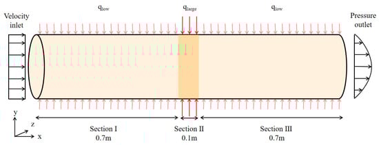
Figure 1.
Schematic diagram of the flow configuration with relevant notations and boundary conditions.
2.2. Control Equations
The liquid and ice particles both are treated as interpenetrative continua in the Euler–Euler approach with interphase momentum and heat exchange. It is assumed that the flow of ice slurry is turbulent as well as incompressible, and that the ice particles are smooth, inelastic, and spherical.
- Continuity equation
Ice slurry is an incompressible fluid. The mass conservation equation satisfies the Navier–Stokes equation (N-S equation), and the expression of each phase equation is shown below:
where is the density, is the local velocity, is the local phase volume fraction, is mass transfer rate caused by melting, and the subscript l represents liquid phase and the subscript s represents solid phase.
The sum of the volume fractions of each phase is one and the relationship is shown as follows:
- Momentum conservation
The momentum equation of ice slurry can still be expressed by the N-S equation. The conservation of momentum equation for each phase is expressed as follows:
For liquid phase
where is pressure, is gravity acceleration, and is the interaction between each phase.
is the pressure-strain tensor of the liquid phase, which expression is shown below:
where is bulk viscosity, is the momentum transfer introduced by the mass exchange due to solid phase melting.
Solid phase
where is the solid pressure derived from granular dynamics theory.
is the solid phase stress, denoted as [38]
is the bulk viscosity of solid phase, which can be formulated as [39]
is the solid shear viscosity which consists of three parts and can be represented as [40]
where is the radial distribution function, is the coefficient of restitution for collisions between particles, is the granular temperature, is the diameter of particles. modifies the probability of particle–particle interaction with the following expression [41].
- Energy conservation
The energy equation for each phase of the ice slurry is expressed as follows:
Solid phase
Liquid phase
where is the enthalpy, is the effective thermal conductivity, is the coefficient of volumetric interphase heat transfer, and is the energy transfer between two phases introduced by mass transfer.
2.3. Turbulence Model
Since the turbulence model (mixture) has higher accuracy and reliability in a wide range of flow fields, the conservation equations are shown as follows:
The constants used in equations are , , , , , , .
2.4. Phase Interfacial Forces
The interaction between solid and liquid phase has a great impact on the solid phase kinetic. Therefore, interfacial effects need to be considered, mainly including drag force, lift force, and virtual mass force.
The expressions are given as follows.
- Drag force
Drag force plays an important role in two-phase flow [42], which is written as
where is the coefficient of interphase momentum exchange.
For [38]
For
is the drag force coefficient and is solid phase Reynolds number. The expressions are as follows
- Lift force
The formulation of lift force is given below [42]
where takes a constant value of 0.2 [43].
2.5. Phase Change Model
Gunn [44] provides a heat transfer correlation for particles moving in liquid, as follows:
is given as follows:
is given as below:
is given as below:
The effective thermal conductivity of the liquid and solid phases in the near-wall region as well as in the main flow region depends on the local IVF and is expressed as follows [45].
- Near-wall region ()
Energy transfer between particles and the wall could be considered based on point contact [46], as follows:
where is the distance from wall, and is the real thermal conductivity of the liquid phase.
- Main flow region ()where is the real thermal conductivity of ice particles.
2.6. Boundary and Initial Conditions
The imposed boundary conditions have been vividly labeled, as shown in Figure 1. A uniform inlet velocity is specified for the inlet boundary as well as an inlet volume fraction. Turbulence intensity and hydraulic diameter are used. The turbulent intensity is taken as 3%, while hydraulic diameter is taken as 16 mm. Pressure outlet is used and specified as 0.1 MPa for the outlet boundary. No-slip condition and constant heat flux are adopted at the wall. In order to save calculation time, the initial conditions of the ice slurry in the flow field are specified as the same as the inlet conditions. The heat flux of the three sections is set to 2 kW/m2, 40 kW/m2, and 2 kW/m2, respectively.
2.7. Numerical Solution Strategy
The three-dimensional numerical model of circular pipe with local large heat flux segment is performed using the commercial CFD solver (FLUENT-2020) to investigate the flow-melt characteristics of ice slurry. In the numerical calculation, the second-order upwind schemes are used to discretize all the governing equations. The equations are solved by phase-couple SIMPLE method. The UDF technology is applied to describe melting and thermal properties change of ice slurry. In the simulations, the time step is taken as 10−3 s and the numerical calculation is considered to converge when all the residuals are lower than 10−4 s and energy residual is lower than 10−8.
3. Numerical Model Validation
Ice particle distribution is more difficult to measure, while solid phase velocity as well as pressure drop are easier to obtain, so most of the previous experimental data revolve around the latter two. In this paper, the solid velocity and pressure drop are chosen as criteria for the validation of the flow model, together verifying the accuracy of the numerical model. Many scholars have made experimental measurements of ice slurry heat transfer properties, mostly under constant wall heat flux, and the heat transfer coefficient is used as the criterion for the validation of the phase change model in this paper.
3.1. Mesh Generation and Grid Independence
In order to improve the calculation accuracy of mesh and reduce the calculation cost, a meshing scheme of hexahedron grid + boundary layer for the horizontal straight pipe is used, as shown in Figure 2.
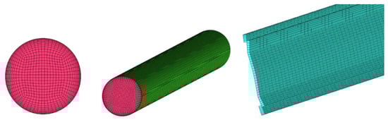
Figure 2.
Schematic diagram of the grid.
The number of grids has a significant impact on the accuracy and time-consumption of numerical calculation, so it is necessary to verify the independence of grids before numerical research. In this paper, seven grid schemes from 0.03 million to 1.6 million grids are compared in terms of solid velocity, IVF distribution, and pressure drop along the central axis, as shown in Figure 3. It can be seen that when the grid number reaches to 1.42 million, it has little effect on the calculation results, so the grid number of 1.42 million is adopted to study the following numerical calculation.
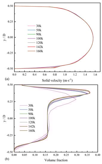
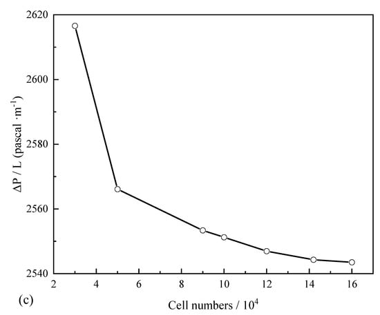
Figure 3.
Comparison of (a) solid-phase velocity distribution (b) IVF distribution (c) pressure drop at different grid densities.
3.2. Sensitivity Validation
In this section, three interphase forces (virtual mass force, drag force, and lift force) are considered to test the sensitivity of the model. The drag force is set as imperative with a model of Gidaspow [38]. The tests are divided into three groups, considering simultaneously virtual mass force, drag force, and lift force, considering only virtual mass force and drag force, and considering only drag force and lift force. Figure 4 shows a comparison in terms of the distribution of solid velocity and IVF along the vertical cross-section of the outlet profile for the three groups. It is observed from Figure 4a that the selection of interphase forces has little effect on the solid velocity distribution. The distribution of solid velocity is more uniform about the center with the addition of lift force. It is seen from Figure 4b that the model considering drag force and lift force behaves the same as the model considering the three interphase forces simultaneously. Since the density difference between solid and liquid phases is not large, the virtual mass force can be neglected. The model considering only virtual mass forces and drag forces shows a different situation, with an increase in IVF in the upper and lower part of the pipe. IVF distribution is significantly influenced by lift force, which makes a smooth transition change in IVF. Therefore, drag forces and lift forces are considered in this numerical model.
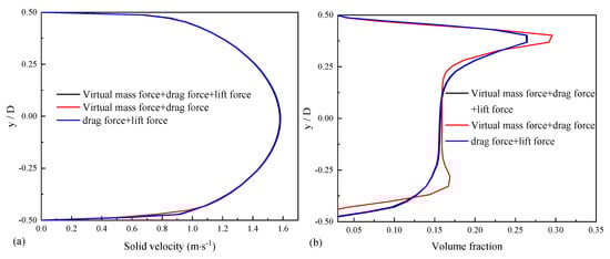
Figure 4.
Distribution of Solid velocity (a) and IVF (b) at x = 1.5 m.
3.3. Validation for Isothermal Ice Slurry Flow
Figure 5a shows a comparison of results between the numerical calculation of the ice slurry solid velocity profile with the experimental results of Vuarnoz [47] obtained by adopting the ultrasonic velocity profiler (UVP) to determine the velocity profile of ice particles. The solid phase velocity appears to be large in the center and small on both sides. As can be seen in Figure 5a, the numerical results are in good agreement with the experimental results, with errors within 10%.
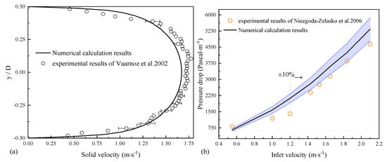
Figure 5.
(a) Comparison of the solid velocity profile of ice slurry with experimental results of Vuarnoz. (b) Comparison of pressure drop of ice slurry with experimental results of Niezgoda-Zelasko [15].
Figure 5b indicates a comparison of results between the numerical calculation of ice slurry pressure drop with experimental results of Niezgoda-Zelasko [15] obtained from many experiments in a 0.016 m diameter horizontal pipe using 15.1% inlet IVF. It is seen from Figure 5b that the general trend of the solid velocity calculated agrees with the experiment values and shows a good linear regularity. The experimental data from the inlet velocity of 1–1.3 m/s shows that the data are not linearly varying, and it is conjectured that this may be caused by measurement errors. Since irregularly shaped ice particles are used in the experiment, consuming a large quantity of kinetic energy due to the collision of ice particles, the pressure drop data are smaller [21]. Neglecting the measurement error points, the remaining data are considered acceptable, mostly falling within 10% of the simulation data, so the numerical model can describe the ice slurry flow well.
3.4. Validation for Non-Isothermal (with Melting) Ice Slurry Flow
Figure 6 shows a comparison of results between the numerical calculation of the local heat transfer coefficient with experimental results of Niezgoda-Zelasko [16] obtain from many experiments in a 0.016 m diameter horizontal pipe using ethanol-water ice slurry with various inlet velocity of 0.5–2.5 m/s and 0.1 mm particle diameter. It can be seen from Figure 6 that the local heat transfer coefficient increases with the inlet velocity due to the increase in turbulence intensity. The calculated results match well with the experimental values, within 5% error from Figure 6.
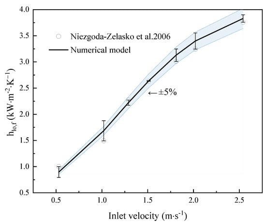
Figure 6.
Comparison of predicted results of heat transfer coefficient with the experimental results of Niezgoda-Zelasko [16].
The local heat transfer coefficient is represented by the equation below:
where is the constant heat flux of the wall, is the temperature of the wall, and is the mean temperature of fluid on the center of cross-section.
4. Results and Discussion
The base case settings, where inlet IVF is 15%, inlet velocity is 1 m/s (Reis = 1950 at the inlet) with qI,III = 2 kW/m2 and qII = 40 kW/m2, are presented and analyzed. The variation of IVF of sections I and II and the whole pipe is represented below as ΔIVF-I, ΔIVF-II, and ΔIVF-all respectively, which is defined as the inlet IVF minus the outlet IVF in the corresponding segment. The recovery characteristic of IVF after passing through the local large heat flux segment is defined as the outlet IVF minus the inlet IVF of Section III. The initial solution consists of 10.3% ethanol aqueous liquid, and the ice particle diameter is fixed at 0.1 mm.
4.1. Distribution Characteristics of Ice Slurry Thermophysical Field
Figure 7 illustrates the distribution characteristics of the physical fields for pressure field, IVF, temperature field, and velocity field at different x cross-sections of the pipe with Re = 1950 and IVFin = 15%. For pressure field, the relative pressure is evenly distributed in the same cross section and gradually decreases along the flow direction. The pressure loss is attributed to the flow resistance caused by the fluid viscosity. Along the flow direction, collision friction between particles and between particles and wall can also lead to pressure loss.
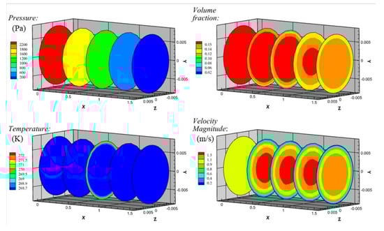
Figure 7.
Distribution of IVF, solid velocity, pressure and temperature at different cross-sections with local large heat flux value of 40 kW/m2.
For ice volume fraction field, it is seen from Figure 7 that the IVF in the mainstream for Section I is not influenced and remains the same as that of the inlet of the pipe. The ice particles absorb heat and melt mainly near the wall. Due to the density difference, the ice particles are suspended above the pipe. Therefore, the reduction of IVF for the lower side is slightly faster than that for the upper side. For Section II, due to the large local heat flux, the ice particles near the wall melt considerably and a liquid phase region appears near the wall along the flow direction. For Section III, under the effect of turbulent dispersion and buoyancy, the mainstream ice slurry is in a squeezing state for the upper near-wall liquid area due to a density difference, while it is in a flashing state for the lower near-wall liquid area. Due to the collision between the particles and the wall, the near-wall liquid phase region is disrupted, and after a certain recovery distance, the distribution of the IVF in the cross section becomes homogeneous again. Figure 8 shows the distribution of IVF along the flowing direction with local large heat flux value of 40 kW/m2 at z = 0. It can be seen clearly that the IVF of upper region remains larger than that of the lower part owing to the two states of the mainstream ice slurry on the liquid area and density difference.
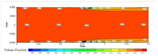
Figure 8.
Distribution of IVF with local large heat flux value of 40 kW/m2 at z = 0.
For temperature fields, it is seen that the near-wall ice slurry has an obvious temperature rise due to the large heat flux in Section II. The ice particles are easily melted, and the liquid phase is warmed up quickly due to the heat obtained. The temperature of the mainstream ice slurry hardly changes due to the weak conduction and most heat is used to melt the near wall ice particles.
For velocity fields, it is seen that the near-wall velocity approaches 0 m/s due to the no-slip boundary condition. The maximum value of the flow velocity and the proportion are gradually reduced along the flow direction due to the friction loss between the ice slurry and the wall and the momentum exchange between the particles in collision. High velocity zone gradually shrinks in a circular shape toward the center of the pipe. The velocity becomes consistent for a large area in the center of outlet of the pipe.
4.2. Effect of Inlet Velocity on the Melting Characteristics of Ice Slurry Flow
In order to investigate how the recovery of ice slurry is influenced by inlet velocity, five kinds of inlet velocity () are applied. The corresponding Reynolds numbers varies between 975 and 4874, the inlet IVF is fixed to 15%, and the local large heat flux is set to 40 kW/m2.
Figure 9a shows a comparison of the axial evolution of IVF for different inlet velocities. It can be seen that ΔIVF-I is strongly influenced by inlet velocity. The amount of melting increases with the decrease of Reynolds numbers. Taking Reynolds number 1950 as delineation, for the low Reynolds number region, the melting amount still increases more even in the low heat flux situation. For Section III, it is found that the IVF rises again along the flow direction which is the recovery phenomenon of IVF of ice slurry flowing after the local large heat flux segment. The gradient of recovery curve for different inlet velocity increases along with the decrease in velocity. For some high velocity conditions, the time for ice slurry flowing through the local large heat flux segment is reduced, the heat absorption is limited, the near-wall liquid phase region cannot be formed, and the introduced IVF variation is very small. Thus, the IVF distribution is less affected. The presence of local large heat flux does not cause much change or damage to the IVF field, so the recovery curve is flat. Under certain low velocity conditions, ice content of Section II is greatly influenced by large heat flux, which lead to the formation of a liquid phase region near the wall. When the velocity is low, the low heat flux also causes relatively obvious melting. The gradient of the recovery curve is still larger, as can be seen from Figure 9a, indicating that the degree of influence on the variation of IVF introduced by the local large heat flux far exceeds that caused by the melting in the low heat flux section.
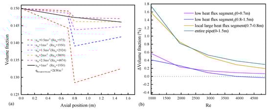
Figure 9.
(a) Axial evolution of IVF (b) ΔIVF of each segment with different Reis.
Figure 9b shows the variation of IVF for each section with different Reynolds number. As can be seen from Figure 9b, ΔIVF-all under the studied conditions is largely determined by the local large heat flux segment. The mainstream ice slurry is less influenced by the heat flux and remains at a relatively high ice concentration, and the decrease in heat flux in section III also leads to a decrease in near-wall melting. Therefore, the IVF of cross-section increases and shows a recovery phenomenon of IVF along the flow direction. It is found that the recovery characteristics of IVF for Section III decrease gradually with increasing Reynolds number.
4.3. Effect of Inlet IVF on the Melting Characteristics of Ice Slurry Flow
To investigate how the recovery characteristics of the ice slurry are affected by the inlet IVF, five kinds of inlet IVF (5%, 10%, 15%, 20%, and 25%) are applied. The heat flux of Section II is set to 40 kW/m2 and the inlet velocity is fixed to 1 m/s.
Figure 10a indicates the comparing of the axial evolution of IVF for different inlet velocities. It is seen that the amount of particle melting in Section II increases with the increase of inlet IVF. Maximum IVF variation is found in Section II. The variation curves of IVF of Section I and Section III are approximated horizontally in Figure 10a. Due to the limited contact heat transfer area and the point contact between the ice particles and the walls, the effect on heat transfer is insignificant even if the collision probability increases with increasing inlet IVF.
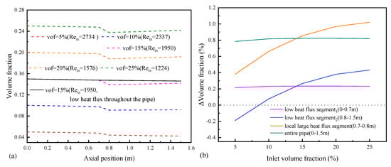
Figure 10.
(a) Axial evolution of IVF with different inlet IVF (b) ΔIVF of each segment with different inlet IVF.
Figure 10b shows variation of IVF for each section with different inlet IVF. For section III, when the inlet IVF is low, the recovery curves of IVF are negative, indicating that the ice particles are continuously melting along the flow direction. It can be presumed that only if the inlet IVF exceeds a certain critical value will it have the recovery characteristic after a local large heat flux section. From Figure 10b, it can be seen that the critical value is approximately 8% for the present boundary conditions. The lower ice content in the mainstream region is not enough to offset the effects of the near-wall liquid phase region caused by the local large heat flux section. Thus, the IVF continues to decrease along the way. The reduction of IVF is 0.215% in Section I and 0.189% in Section III, which becomes smaller after the large heat flux section. This also reveals the recovery characteristics of volume fraction of ice slurry. As the inlet IVF increases, the recovery of the IVF becomes positive and increases accordingly. It is worth noting that ΔIVF-all remains almost constant. It can be seen that the inlet IVF is not an important factor for the amount of melting of the pipe compared to the inlet velocity. From the gradient of the corresponding pipe segment curve, it is clear that the inlet IVF has the same influence on ΔIVF-II and the recovery of IVF.
At the inlet IVF of 15%, it is observed that ΔIVF-all and ΔIVF-II are almost the same. ΔIVF-all is smaller or larger than ΔIVF-II when the inlet IVF is greater or less than 15%. Therefore, it is necessary to transport ice slurry with an ice content greater than 15% to minimize melting losses due to heat leakage through pumps and other connected components.
4.4. Effect of Local Heat Flux on the Melting Characteristics of Ice Slurry Flow
Figure 11 shows the IVF variation of ice slurry passing through each section with different values of the heat flux multiplier in section II, where the values of the heat flux multiplier in section II are 5, 10, 20, 30, 40, and 50 times the heat flux in section I, at an inlet velocity of 1 m/s and an inlet IVF of 15%, respectively. It can be seen that as the local large heat flux increases, the IVF decreases along the flow direction and the melting of ice particles near the walls increases. After the heat flux is greater than 20 times, the liquid phase zone is observed near the wall, which can be seen in Figure 8. From Figure 11a, it can also be observed that there is a significant IVF recovery along the Section III. As the local large heat flux increases, the gradient of the recovery curves first increases and then changes slightly. It is presumed that the gradient of the recovery curve is more dependent on the liquid phase region, and the gradient is essentially constant after the appearance of the liquid phase region (i.e., after the local large heat flux is greater than 20 times)
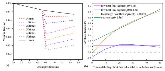
Figure 11.
(a) Axial evolution of IVF (b) ΔIVF of each segment at different multiples of local large heat flux section.
Figure 11b indicates the variation of IVF for each section with different local large heat flux. It can be seen more directly that the IVF recovery value increases first with increasing heat flux and then remains essentially constant. It can be deduced that increasing the heat flux has a negligible effect on IVF recovery when the local large heat flux exceeds a certain value. The ΔIVF-all increases linearly with the increasing multiplier.
Figure 12 shows the distribution of IVF for five local large heat flux multiples (5, 10, 20, 40, 50 times) at different x cross-sections. The inlet and outlet of the local large heat flux segment and three cross-sections of Section III are chosen to display the IVF. It can be seen from the legend of Figure 12 that the minimum value of IVF gradually increases along the flow direction in Section III. This indicates that the proportion of liquid phase in the near-wall region gradually decreases, and the cross-sectional IVF has a tendency to be re-uniform. From Figure 12c, under shear stress action as well as the effect of mixing, the near-wall liquid phase region is disrupted and the IVF in the near-wall region is increased. While the IVF around the mainstream decreases, the area of high ice content of the mainstream region shrinks toward the center. It is presumed from Figure 12d,e that the boundary layer is re-established after x = 1.267 m and the distribution of IVF tends to remain stable. Therefore, after the large heat flux, the IVF of the ice slurry demonstrates re-uniform distribution along the cross section.
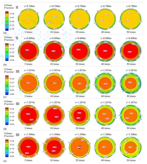
Figure 12.
Distribution of IVF for fivelocal large heat flux multiples (5, 10, 20, 40, 50 times) at different x cross-sections (a) 0.7 m, (b) 0.8 m, (c) 1.033 m, (d) 1.267 m, (e) 1.5 m.
Figure 13 shows the axial variation of IVF at six monitoring points on the same vertical line for six large heat flux multiples (5, 10, 20, 40, 50 times, respectively). In order to focus on the re-uniform of ice volume fraction distribution after passing through the local large heat flux segment, six near wall monitoring points are selected for comparison. The boundary layer is destroyed by the melting near the wall. A certain distance is needed to weaken the effect of inhomogeneous stratification due to melting, when the boundary layer is re-established and the distribution of IVF returns to a uniform state. Owing to slight difference in ice slurry in the mainstream, the near-wall region is applied to determine the re-uniformity of ice fraction distribution, and ice fraction distribution at x = 1.48 m is chosen as criterion. It is stipulated that a relative error within 2% is considered that the distribution of IVF is returned to uniformity. Relative error is defined as . In the case of different multiples, the axial position corresponding to the re-uniformization of 5 and 10 times is roughly x = 1.1 m, for 20 times is roughly x = 1.35 m, and for 30, 40 and 50 times are roughly x = 1.4 m. It is found that as the multiplicity of large heat flux increases, there-uniformization length becomes longer.
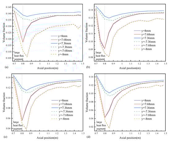
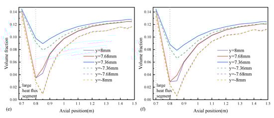
Figure 13.
Axial variation of IVF at six monitoring points on the same vertical line for six large heat flux multiples (a) 5, (b) 10, (c) 20, (d) 30, (e) 40, (f) 50 times.
The firm line represents the upper data points, while the dashed line represents the lower data points. It is seen clearly that the IVF of the upper part is larger than that of the lower part due to the density difference. It is interesting to find that the minimum value of IVF does not appear at the outlet of the local large heat flux section but has a certain delay, as seen in Figure 13, basically at x = 0.85 m. It can be found that there is a relatively obvious recovery of the IVF in the x cross-section after the local large heat flux section, as well as a re-uniformity.
Figure 14 indicates the average heat transfer coefficient for each section at different multiples of local large heat flux. It can be noticed that in Section II, the average heat transfer coefficient increases with the increasing multiples of heat flux due to the near-wall melting. This is because the boundary is severely damaged, which strengthens the heat and mass transfer between the mainstream region and the near-wall region. The average heat transfer coefficient of Section III changes slightly for 5–20 multiples while decrease with the increase of heat flux for multiples bigger than 20. This is presumed to be caused by the thermophysical properties of the ice slurry as well as changes in the distribution of ice particles [32]. The viscosity as well as the effective thermal conductivity of the ice slurry increases with increasing ice concentration. In Section III, the temperature of the ice slurry increases, the IVF decreases, and the viscosity decreases, leading to a corresponding increase in the heat transfer coefficient. However, the effective thermal conductivity decreases with decreasing ice content, and the heat transfer coefficient should decrease accordingly. From Figure 14, it can be seen that when the heat flux is greater than 20 times, the heat transfer coefficient decreases. From this, it can be inferred that the effective thermal conductivity may bring more influence than the viscosity on average heat transfer coefficient.
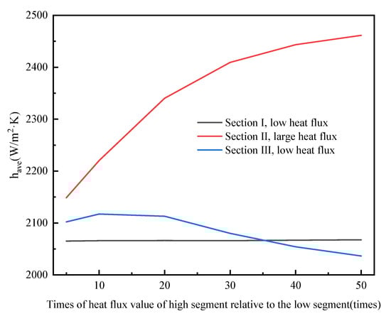
Figure 14.
The average heat transfer coefficient for each section at different multiples of local large heat flux.
5. Conclusions
The flow-melting characteristics are simulated for ice slurry in a straight horizontal pipe with a localized large heat flux section. The flow-melt characteristic of ice slurry under different boundary conditions is obtained. Axial recovery and re-uniformization of distribution of IVF after local large heat flux segment are investigated. The conclusions drawn are as follows.
- (1)
- A 3D Eulerian-Eulerian model based on the granular kinetics theory considering the turbulence model and phase change is developed, which can accurately describe the heat transfer characteristics of ice slurry.
- (2)
- When the local large heat flux is 20 times higher than the low heat flux, a liquid phase region will appear near the wall.
- (3)
- After passing through the local large heat flux segment, the IVF and the particle uniformity of the cross section have recovery characteristics due to shear stress action. The degree of recovery is determined by the degree of disruption of the IVF field by the local large heat flux.
- (4)
- The re-uniformization length increases with the increasing local large heat flux. Interestingly, the minimum value of IVF does not appear at the outlet of the local large heat flux section, but with a certain delay.
- (5)
- The average heat transfer coefficient of the local large heat flux segment increases due to the boundary damage.
Author Contributions
Conceptualization, F.X. and W.G.; methodology, W.G. and Y.Z.; software, W.G.; validation, W.G.; formal analysis, F.X. and W.G.; investigation, W.G.; resources, W.G.; data curation, W.G.; writing—original draft preparation, F.X. and W.G.; writing—review and editing, F.X. and W.G.; visualization, W.G. and Y.Z.; supervision, F.X.; project administration, F.X.; funding acquisition, F.X. All authors have read and agreed to the published version of the manuscript.
Funding
This research was funded by National Natural Science Foundation of China (52276018), China Postdoctoral Science Foundation (2021T140538, 2020M673391, 2018M633505), and Fundamental Research Funds for the Central Universities (XZY012020074).
Data Availability Statement
No new data were created or analyzed in this study. Data sharing is not applicable to this article.
Conflicts of Interest
The authors declare no conflict of interest.
References
- Ghoreishi-Madiseh, S.A.; Kuyuk, A.F.; Kalantari, H.; Sasmito, A.P. Ice versus battery storage; a case for integration of renewable energy in refrigeration systems of remote sites. Energy Procedia 2019, 159, 60–65. [Google Scholar] [CrossRef]
- Rayhan, F.A.; Pamitran, A.S.; Yanuar; Patria, M.P. Investigating the performance of ice slurry system and the growth of ice crystals using seawater. J. Mech. Sci. Technol. 2020, 34, 2627–2636. [Google Scholar] [CrossRef]
- Youssef, Z.; Delahaye, A.; Huang, L.; Trinquet, F.; Fournaison, L.; Pollerberg, C.; Doetsch, C. State of the art on phase change material slurries. Energy Convers. Manag. 2013, 65, 120–132. [Google Scholar] [CrossRef]
- Kauffeld, M.; Kawaji, M.; Peter, E.W. Handbook on Ice Slurries; International Institute of Refrigeration: Paris, France, 1798. [Google Scholar]
- Kauffeld, M.; Gund, S. Ice slurry—History, current technologies and future developments. Int. J. Refrig. 2019, 99, 264–271. [Google Scholar] [CrossRef]
- Wang, J.; Wang, S.; Zhang, T.; Battaglia, F. Numerical and analytical investigation of ice slurry isothermal flow through horizontal bends. Int. J. Refrig. 2018, 92, 37–54. [Google Scholar] [CrossRef]
- Ma, F.; Zhang, P. A review of thermo-fluidic performance and application of shellless phase change slurry: Part 1—Preparations, properties and applications. Energy 2019, 189. [Google Scholar] [CrossRef]
- Kauffeld, M.; Wang, M.J.; Goldstein, V.; Kasza, K.E. Ice slurry applications. Int. J. Refrig. 2010, 33, 1491–1505. [Google Scholar] [CrossRef] [PubMed]
- Ma, F.; Zhang, P. A review of thermo-fluidic performance and application of shellless phase change slurry: Part 2—Flow and heat transfer characteristics. Energy 2020, 192. [Google Scholar] [CrossRef]
- Wang, J.; Battaglia, F.; Wang, S.; Zhang, T.; Ma, Z. Flow and heat transfer characteristics of ice slurry in typical components of cooling systems: A review. Int. J. Heat Mass Transfer. 2019, 141, 922–939. [Google Scholar] [CrossRef]
- Wang, J.; Wang, S.; Zhang, T.; Liang, Y. Numerical investigation of ice slurry isothermal flow in various pipes. Int. J. Refrig. 2013, 36, 70–80. [Google Scholar] [CrossRef]
- Grozdek, M.; Khodabandeh, R.; Lundqvist, P.; Palm, B.; Melinder, Å. Experimental investigation of ice slurry heat transfer in horizontal tube. Int. J. Refrig. 2009, 32, 1310–1322. [Google Scholar] [CrossRef]
- Grozdek, M.; Khodabandeh, R.; Lundqvist, P. Experimental investigation of ice slurry flow pressure drop in horizontal tubes. Exp. Therm. Fluid Sci. 2009, 33, 357–370. [Google Scholar] [CrossRef]
- Lee, D.W.; Yoon, E.S.; Joo, M.C.; Sharma, A. Heat transfer characteristics of the ice slurry at melting process in a tube flow. Int. J. Refrig. 2006, 29, 451–455. [Google Scholar] [CrossRef]
- Niezgoda-Żelasko, B.; Zalewski, W. Momentum transfer of ice slurry flows in tubes, experimental investigations. Int. J. Refrig. 2006, 29, 418–428. [Google Scholar] [CrossRef]
- Niezgoda-Żelasko, B. Heat transfer of ice slurry flows in tubes. Int. J. Refrig. 2006, 29, 437–450. [Google Scholar] [CrossRef]
- Kumano, H.; Asaoka, T.; Sawada, S. Effect of initial aqueous solution concentration and heating conditions on heat transfer characteristics of ice slurry. Int. J. Refrig. 2014, 41, 72–81. [Google Scholar] [CrossRef]
- Mi, S.; Cai, L.; Ma, K.; Liu, Z. Investigation on flow and heat transfer characteristics of ice slurry without additives in a plate heat exchanger. Int. J. Heat Mass Transf. 2018, 127, 11–20. [Google Scholar] [CrossRef]
- Ohira, K.; Kurose, K.; Okuyama, J.; Saito, Y.; Takahashi, K. Pressure drop reduction and heat transfer deterioration of slush nitrogen in triangular and circular pipe flows. Cryogenics 2017, 81, 60–75. [Google Scholar] [CrossRef]
- Li, Y.; Jin, T.; Wu, S.; Wei, J.; Xia, J.; Karayiannis, T.G. Heat transfer performance of slush nitrogen in a horizontal circular pipe. Therm. Sci. Eng. Prog. 2018, 8, 66–77. [Google Scholar] [CrossRef]
- Hu, J.; Tao, T. Numerical investigation of ice pigging isothermal flow in water-supply pipelines cleaning. Chem. Eng. Res. Des. 2022, 182, 428–437. [Google Scholar] [CrossRef]
- Gao, Y.; Ning, Y.; Xu, M.; Wu, C.; Mujumdar, A.S.; Sasmito, A.P. Numerical investigation of aqueous graphene nanofluid ice slurry passing through a horizontal circular pipe: Heat transfer and fluid flow characteristics. Int. Commun. Heat Mass Transf. 2022, 134. [Google Scholar] [CrossRef]
- Cai, L.; Mi, S.; Luo, C.; Liu, Z. Numerical investigation on heat and mass transfer characteristics of ice slurry in pulsating flow. Int. J. Heat Mass Transf. 2022, 189. [Google Scholar] [CrossRef]
- Yadav, S.K.; Ziyad, D.; Kumar, A. Numerical investigation of isothermal and non-isothermal ice slurry flow in horizontal elliptical pipes. Int. J. Refrig. 2019, 97, 196–210. [Google Scholar] [CrossRef]
- Xu, L.; Huang, C.-X.; Huang, Z.-F.; Sun, Q.; Li, J. Numerical simulation of flow and melting characteristics of seawater-ice crystals two-phase flow in inlet straight pipe of shell and tube heat exchanger of polar ship. Heat Mass Transf. 2018, 54, 3345–3360. [Google Scholar] [CrossRef]
- Jin, T.; Li, Y.; Wu, S.; Wei, J. Flow field and friction factor of slush nitrogen in a horizontal circular pipe. Cryogenics 2018, 91, 87–95. [Google Scholar] [CrossRef]
- Jin, T.; Li, Y.J.; Liang, Z.B.; Lan, Y.Q.; Lei, G.; Gao, X. Numerical prediction of flow characteristics of slush hydrogen in a horizontal pipe. Int. J. Hydrog. Energy 2017, 42, 3778–3789. [Google Scholar] [CrossRef]
- Shi, X.J.; Zhang, P. Two-phase flow and heat transfer characteristics of tetra-n-butyl ammonium bromide clathrate hydrate slurry in horizontal 90° elbow pipe and U-pipe. Int. J. Heat Mass Transf. 2016, 97, 364–378. [Google Scholar] [CrossRef]
- Zhang, P.; Shi, X.J. Thermo-fluidic characteristics of ice slurry in horizontal circular pipes. Int. J. Heat Mass Transfer. 2015, 89, 950–963. [Google Scholar] [CrossRef]
- Li, Y.; Wang, S.; Wang, J.; Zhang, T. CFD Study of Ice Slurry Heat Transfer Characteristics in a Straight Horizontal Tube. Procedia Eng. 2016, 146, 504–512. [Google Scholar] [CrossRef]
- Onokoko, C.L.; Galanis, N. Stratification in Isothermal Ice-Slurry Pipe Flow. In Proceedings of the ASME International Mechanical Engineering Congress and Exposition, San Diego, CA, USA, 15–21 November 2013. [Google Scholar]
- Onokoko, C.L.; Galanis, N.; Poncet, S.; Poirier, M. Heat transfer of ice slurry flows in a horizontal pipe: A numerical study. Int. J. Therm. Sci. 2019, 142, 54–67. [Google Scholar] [CrossRef]
- Onokoko, L.; Poirier, M.; Galanis, N.; Poncet, S. Experimental and numerical investigation of isothermal ice slurry flow. Int. J. Therm. Sci. 2018, 126, 82–95. [Google Scholar] [CrossRef]
- Suzuki, K.; Kawasaki, T.; Asaoka, T.; Yoshino, M. Numerical simulations of solid–liquid and solid–solid interactions in ice slurry flows by the thermal immersed boundary–lattice Boltzmann method. Int. J. Heat Mass Transf. 2020, 157. [Google Scholar] [CrossRef]
- Bordet, A.; Poncet, S.; Poirier, M.; Galanis, N. Flow visualizations and pressure drop measurements of isothermal ice slurry pipe flows. Exp. Therm. Fluid Sci. 2018, 99, 595–604. [Google Scholar] [CrossRef]
- Bordet, A.; Poncet, S.; Poirier, M.; Galanis, N. Advanced numerical modeling of turbulent ice slurry flows in a straight pipe. Int. J. Therm. Sci. 2018, 127, 294–311. [Google Scholar] [CrossRef]
- Languri, E.M.; Rokni, H.B. Flow of Microencapsulated Phase Change Material Slurry through Planar Spiral Coil. Heat Transf. Eng. 2017, 39, 977–984. [Google Scholar] [CrossRef]
- Gidaspow, D. Multiphase Flow and Fluidization: Continuum and Kinetic Theory Descriptions, 1st ed.; Academic Press: New York, NY, USA, 1994. [Google Scholar]
- Lun, C.K.K.; Savage, S.B.; Jeffrey, D.J.; Chepurniy, N. Kinetic theory for grannular flow: Inelastic particles in Couette flow and slightly inelastic particles in general flow field. J. Fluid. Mech. 1984, 140, 223–256. [Google Scholar] [CrossRef]
- Syamlal, M.; Brien, T.J.O. Computer simulation of bubbles in a fluidized bed. AlChE Symp. Ser. 1989, 85, 22–31. [Google Scholar]
- Ogawa, S.; Umemura, A.; Oshima, N. On the equation of fully fluidized granular materials. Appl. Math. Phys. 1980, 31, 483. [Google Scholar] [CrossRef]
- Ekambara, K.; Sanders, R.S.; Nandakumar, K.; Masliyah, J.H. Hydrodynamic simulation of horizontal slurry pipeline flow using ANSYS-CFX. Ind. Eng. Chem. Res. 2009, 48, 8159–8171. [Google Scholar] [CrossRef]
- Tomiyama, A. Drag, lift and virtual mass forces acting on a single bubble. In Proceedings of the Third International Symposium on Two-Phase Flow Model and Experiment, Pisa, Italy, 22–24 September 2004; pp. 22–24. [Google Scholar]
- Gunn, D.J. Transfer of heat or mass to particles in fixed and fluidised beds. Int. J. Heat Mass Transf. 1978, 21, 467–476. [Google Scholar] [CrossRef]
- Zehner, P.; Schlünder, E.U. Wärmeleitfähigkeit von Schüttungen bei mäßigen Temperaturen. Chem. Ing. Tech. 1970, 42, 933–941. [Google Scholar] [CrossRef]
- Legawiec, D.Z. Structure, voidage, and effective thermal conductivity of solids within near-wall region of beds packed with spherical pellets in tubes. Chem. Eng. Sci. 1984, 49, 2513–2520. [Google Scholar] [CrossRef]
- Vuarnoz, D.; Sari, O.; Egolf, P.W.; Liardon, H. Ultrasonic velocity profiler UVP-XW for iceslurry flow characterisation. In Proceedings of the EPFL International Symposium on Ultrasonic Doppler Methods for Fluid Mechanics and Fluid Engineering, Lausanne, Switzerland, 9–11 September 2002. [Google Scholar]
Disclaimer/Publisher’s Note: The statements, opinions and data contained in all publications are solely those of the individual author(s) and contributor(s) and not of MDPI and/or the editor(s). MDPI and/or the editor(s) disclaim responsibility for any injury to people or property resulting from any ideas, methods, instructions or products referred to in the content. |
© 2023 by the authors. Licensee MDPI, Basel, Switzerland. This article is an open access article distributed under the terms and conditions of the Creative Commons Attribution (CC BY) license (https://creativecommons.org/licenses/by/4.0/).