Machine Learning Predictions of Electricity Capacity

Abstract

This research applies machine learning methods to build predictive models of Net Load Imbalance for the Resource Sufficiency Flexible Ramping Requirement in the Western Energy Imbalance Market. Several methods are used in this research, including Reconstructability Analysis, developed in the systems community, and more well-known methods such as Bayesian Networks, Support Vector Regression, and Neural Networks. The aims of the research are to identify predictive variables and obtain a new stand-alone model that improves prediction accuracy and reduces the INC (ability to increase generation) and DEC (ability to decrease generation) Resource Sufficiency Requirements for Western Energy Imbalance Market participants. This research accomplishes these aims. The models built in this paper identify wind forecast, sunrise/sunset and the hour of day as primary predictors of net load imbalance, among other variables, and show that the average size of the INC and DEC capacity requirements can be reduced by over 25% with the margin of error currently used in the industry while also significantly improving closeness and exceedance metrics. The reduction in INC and DEC capacity requirements would yield an approximate cost savings of $4 million annually for one of nineteen Western Energy Imbalance market participants. Reconstructability Analysis performs the best among the machine learning methods tested.

1. Introduction

The California Independent System Operator (CAISO) Western Energy Imbalance Market (WEIM) is an intra-hour electricity market with a footprint across much of the Western US, including participants in California, the Pacific Northwest, the Southwest, and other areas. The market aims to balance supply and demand of electricity across this footprint on a 5-min basis in the most economical way while satisfying a variety of constraints [1]. Each participant must enter the market each hour with sufficient energy for its anticipated electricity demand (commonly referred to as “load”) and also with capacity to meet some amount of uncertainty in supply and demand. Prior research has shown that variable generation like wind and solar, and load forecasts [2,3,4,5] are primary drivers of supply and demand uncertainty. The focus of this paper is on the appropriate amount of uncertainty that the CAISO should plan for each WEIM participant; more precisely, on the difference between actual supply and demand in a given time period that a WEIM participant should be able to compensate for with its INC and DEC capacities without assistance from other WEIM participants. This difference between supply and demand (commonly referred to as “imbalance”) is the dependent variable (DV, observed net load imbalance) being predicted in this study. (This DV is described section titled “Data”.).

In order to establish the pool of generators that can be adjusted up or down, participants bid into the market INC and DEC capacity on an hourly basis to indicate the amount they are willing to adjust energy output up or down in the coming hour (along with a price for such adjustments). INC capacity is the capacity to respond to situations when demand exceeds supply. It is the ability to increase energy output within a certain timeframe and is deployed when loads come in higher than expected and/or generators produce lower energy than expected. Participants called upon to increase generation are compensated for this deployment of energy. DEC capacity is the inverse, the capacity to respond to situations when supply exceeds demand. Specifically, it is the ability of generators to decrease energy output within a certain timeframe, called upon by the market operator and deployed by the participant when loads come in lower than expected and/or generators produce more energy than expected. Participants called upon to decrease generation save money because their sale to serve load is served by a cheaper market resource.

To participate fully in the WEIM for each hour, WEIM participants must meet four separate Resource Sufficiency Tests [6]. Meeting these requirements provides the entire market with access to a large enough pool of adjustable generation and guarantees that participants are not relying on other market participants for their INC and DEC capacity needs. This pool of adjustable capacity ensures that generation supply can reliably meet load for all market participants in every time interval.

The Flexible Ramp Sufficiency Test (FRST) is one of the four Resource Sufficiency Tests [6,7]. This test establishes the minimum amount of INC and DEC reserves a participant must bid into the market in order to participate. Participants can bid more if they choose. This test is the focus of the analysis in this paper. The FRST, specifically the uncertainty component of the FRST, currently requires a participant to bid an amount of DEC capacity equal to the 2.5 percentile of “observed net load imbalance” (which is Variable 1, the dependent variable, defined further in the section titled “Data”) for that participant, for the given hour, over the prior 40 weekdays, and to bid an amount of INC capacity equal to the 97.5 percentile over the same period. For weekends, the 2.5 and 97.5 percentiles are determined for the given hour, from the prior 20 weekend days [7]. Setting the threshold at this level assumes that recent historical observations of net load imbalance are a good predictor of the potential range of imbalance in a coming hour. The goal of this approach is to create an INC and DEC upper and lower bound to ensure each participant is bringing enough INC and DEC capacity to support their historical net load imbalance. This approach is referred to as the Industry Model throughout the paper.

Prior research has shown that probabilistic methods like Bayesian Networks [4] and Monte Carlo simulation [2] improved the accuracy of net load imbalance forecasts. Further, prior research has shown different ML methods have advantages and disadvantages in predicting wind energy, solar energy and load forecasts [8].

Reconstructability Analysis (RA), Bayesian Networks (BN), Support Vector Regression (SVR), and Neural Networks (NN) are machine learning methodologies. RA and BN are both probabilistic graphical modeling methodologies and SVR and NN are other more commonly used machine learning methods. These four methods are applied in this paper to data provided by the Bonneville Power Administration to build point estimate prediction models of observed net load imbalance, the DV (point estimate prediction models are described in the section titled “Results of DV prediction: comparing ML methods to Industry Model”). All of these methods underwent a 5 fold cross validation to ensure each model generalized well to new data. Midpoint predictions of the Industry Model and machine learning methods are compared in the section titled “Results of DV prediction: comparing ML methods to Industry Model” using three statistics: R squared, mean squared error, and mean absolute error.

The primary purpose of the first part of this study, where we used ML methods to build point estimate predictions of observed net load imbalance was to pick a good ML method for the second part of the study where, more importantly, INC and DEC predictions are made and compared to the Industry Model. That is, we do not here undertake a general comparison of the four ML methods, which would require applying them to multiple data sets; our aim in the first part of the study is primarily to identify a promising ML method for INC and DEC predictions.

The results of the point estimate predictions from the first part of the study show that three of the four methods do significantly better than the current Industry Model [7], and RA performed best overall; and the results of the second part of the study where RA is applied to make INC and DEC predictions show that the RA Model does significantly better than the Industry Model.

Metrics used to compare the RA INC and DEC prediction model to the Industry Model operationalize the general definitions published by the CAISO [9] and are: Average Requirement (the average INC and DEC requirement over all observations in the dataset), Coverage (a measure that is the inverse of error, where error is how many times actual imbalance is outside the INC and DEC requirement), Closeness (how close the actual imbalance is to the INC and DEC requirement, whether greater or less than these requirements), and Exceedance (when, more specifically, imbalance is greater than the INC or DEC requirement, how much does it exceed the INC or DEC requirement). These metrics are described in detail in the section titled “Metrics for comparing the INC and DEC prediction efficacy”.

Of all the analyses in the paper, the results of the RA Model INC and DEC predictions have the greatest potential practical significance for the CAISO and WEIM participants. As shown in the test described in the section titled “Industry Model and RA Model INC and DEC prediction results,” the RA Model allows the FRST INC and DEC Average Requirement (the average amount of INC and DEC reserves that must be held) to be reduced by a total of 150.9 MW (To provide a sense of the scale of this reduction, 1 MW (one million watts) can power between 400 and 900 homes [10] depending on a number of factors), a 25.4% total reduction; specifically, 62.7 MW for INC reserves, a 23.0% reduction, and 88.2 MW DEC reserves, a 27.3% reduction while producing the same level of Coverage (the inverse of error) as the Industry Model. Additionally, Closeness and Exceedance metrics are also improved by the RA Model. These findings show that if the best RA model were used, the CAISO can retain the same Coverage as it has currently, while significantly lowering the INC and DEC requirement for WEIM participants. Ultimately this has benefit to both the CAISO and WEIM participants in the form of lower cost. Conservatively, reducing the reserve requirement by this amount would result in approximately $4 million (INC savings would be $168/MW − day × 365 days × 62.7 MW = $3.84 million. DEC savings would be $12/MW − day × 365 days × 88.2 MW = $386 thousand) in annual savings for the Bonneville Power Administration which is one of nineteen WEIM participants and which is the focus of the data analysis in this paper.

The following sections of this paper are organized as follows. The materials and methods section provides a description of the data used to perform the analysis and describes the four machine learning methods applied to the data as well as the Industry Model that is in current use. Results are then reported in two parts: an across-method comparisons of point estimate results and the RA Model INC and DEC predictions compared to the Industry Model. The last sections offer a discussion and conclusion focused on key findings and observations, and future possible research extensions.

2. Materials and Methods

2.1. Data

The data used in this analysis came from the Bonneville Power Administration which is a wholesale electric utility that began participation in the WEIM in the summer of 2022. The data is time series, in 15 min increments from January of 2014 to December of 2018. There are 172,175 observations, and there are no missing data. There are 22 independent variables (IV) and one dependent variable (DV). 18 of the IVs are continuous, 4 are discrete. The DV is continuous.

Table 1. Variable Names and Definitions.

Variable Number	Variable Name	Variable Name Single Letter Abbreviation	DV or IV	Continuous or Discrete	For RA/BN, Number of Bins	Time Lag	Short Description
1	NLFCErrorBoth_A	Z	DV	Continuous	6	0	Observed Net Load Imbalance. Positive values represent use of INC reserves to meet load requirements. Negative values represent use of DEC reserves to meet load requirements.
2	LoadRTD	A	IV	Continuous	3	48 h lag	Five-minute load measurement used in EIM 5-min market optimization.
3	VERRTD	B	IV	Continuous	3	48 h lag	Five-minute VER measurement used in EIM 5-min market optimization.
4	Net Load RTD	C	IV	Continuous	3	48 h lag	Five-minute measurement of load net VERs. Equal to LoadRTD–VERRTD.
5	NLMaxRTD	D	IV	Continuous	3	48 h lag	For each 15-min interval, the maximum of the three 5-min Net Load RTD values.
6	NLMinRTD	E	IV	Continuous	3	48 h lag	For each 15-min interval, the minimum of the three 5-min Net Load RTD values.
7	LoadFMM	F	IV	Continuous	3	48 h lag	Fifteen-minute load forecast used in EIM 15-min market optimization.
8	VERFMM	G	IV	Continuous	3	48 h lag	Fifteen-minute VER forecast used in EIM 15-min market optimization.
9	NLFMM	H	IV	Continuous	3	48 h lag	Fifteen-minute forecast of load net VERs. Equal to LoadFMM–VERFMM.
10	VERFCFHfrtegt	I	IV	Continuous	3	0	Forecast of wind generation for the 15 min time period the DV is being predicted, forecast made 48 h prior
11	VERFCFHsvntwo	J	IV	Continuous	3	0	Forecast of wind generation for the 15 min time period the DV is being predicted, forecast made 72 h prior
12	VERFCFHninsx	K	IV	Continuous	3	0	Forecast of wind generation for the 15 min time period the DV is being predicted, forecast made 96 h prior
13	VERFCFHonetwty	L	IV	Continuous	3	0	Forecast of wind generation for the 15 min time period the DV is being predicted, forecast made 120 h prior
14	HLH/LLH	M	IV	Discrete	2	0	Heavy Load Hour—6 a.m. to 10 p.m., Monday through Saturday, Light Load Hour—10 p.m. to 6 a.m. Monday through Saturday and all day Sunday.
15	Season	N	IV	Discrete	4	0	Winter (Dec. 1–Feb. 28), Spring (Mar. 1 to May 31), Summer (June 1–Aug. 31), Fall (Sept. 1–Nov. 30)
16	Sunrise/Sunset	O	IV	Discrete	2	0	Sunrise (5 a.m.–7 a.m.), Sunset (5 p.m.–7 p.m.)
17	Hour of Day (2hr groups)	P	IV	Discrete	12	0	hours of the day grouped into 2 h groups, e.g., hours 1 and 2 grouped as 1, hours 3 and 4 grouped as 2, etc.)
18	NLFCErrorBothx2x1dayx	Q	IV	Continuous	3	48 h lag	1 day average of the DV “NLFCErrorBoth_A”
19	NLFCErrorBothx2x20dayx	R	IV	Continuous	3	48 h lag	20 day average of the DV “NLFCErrorBoth_A”
20	LoadRTD 24 Hr Avg	S	IV	Continuous	3	48 h lag	24 h average of IV “Load RTD”
21	LoadRTD24hrstdv	T	IV	Continuous	3	48 h lag	24 h standard deviation of IV “Load RTD”
22	LoadRTD 7 day Avg	U	IV	Continuous	3	48 h lag	7 day average of IV “Load RTD”
23	LoadRTD7daystdv	V	IV	Continuous	3	48 h lag	7 day standard deviation of IV “Load RTD”

below lists the IVs and the DV, including characteristics about each variable and a short definition.

The DV (NLFCErrorBoth_A which is synonymous with the term “observed net load imbalance”) is the difference between demand and supply (net load—generation), of electricity measured every 15 min. Positive values represent load in excess of generation and negative values represent generation in excess of load. The FRST establishes an INC and DEC range for each hour for each WEIM participant. For all the analysis in this paper, INC and DEC predictions described in the section titled “Results of INC/DEC prediction: comparing RA Model to Industry Model” and midpoint predictions described in the section titled “Results of DV prediction: comparing machine learning methods to Industry Model” are made in 15 min increments. That is, when any one of the machine learning methods makes a forecast for the following day, for a given hour, it is for a given 15 min increment within that hour, and the actual observed net load imbalance for that specific 15 min increment is compared to the prediction made for the same 15 min increment. For the Industry Model, the INC and DEC predictions and mid-point predictions for a given hour are the same for each of the four 15 min increments within that hour.

The IVs were selected based upon expert judgement gathered by surveying electrical engineers from the Bonneville Power Administration who are familiar with the variables that impact the DV, the Resource Sufficiency Tests, and WEIM operating requirements. In addition, in a survey of prior literature, Wind Forecast, Solar and Load Forecasts were shown to be primary predictors of net load imbalance [2,3,4,5] and are included the dataset in Table 1. The IV list of Table 1 is not exhaustive, as there may be other predictive variables that were not included, but it does provide a robust sampling of potentially predictive IVs.

Most IVs were lagged 48 h from the DV. Exceptions were time based IVs, for example the IV “Season” which represents one of four seasons (Winter, Spring, Summer, Fall). Another exception was “Wind Forecast” because the forecast was produced at least 48 h in advance. Lagging most variables was necessary in order to replicate the FRST INC and DEC prediction process (and the information available at the time the forecast is made) of the market operator (CAISO). The market operator needs to make the forecast (establishing the INC and DEC reserves requirement) at least 24 h in advance of the actual occurrence in order to be able to tell the WEIM participants what their minimum INC and DEC requirement is. A 48 h lag of the IVs was chosen in this study to be conservative, so that the data would definitely be available in time for the operator to use in the forecast establishing the INC and DEC requirement. Thus it is not unreasonable to expect that if the variables were lagged only 24 h, the machine learning method results would be even better than what is reported here.

Time based variables do not need to be lagged because they are known exactly. For example, what “Season” is 48 h ahead is known. The operator also knows, for example, what “hour of the day” is 48 h ahead. Similarly, for the Wind Forecast, the operator has a forecast of Wind Generation 48 h ahead, 72 h ahead, 96 h ahead, and 120 h ahead. All these forecast time frames are at, or greater, than the 48 h forecast the operator makes.

For both RA and BN, continuous data were binned into equal count bins, i.e., there were roughly an equal number of samples in each bin. For most IVs, three bins were used, i.e., low, medium, and high. By contrast, for SVR and NN, the continuous values were used. For all methodologies, the data was randomly divided into five equal folds (A, B, C, D, E) with 34,435 samples each. The original data had N = 5 × 34,435 cases (172,175), each case separated from what preceded and what followed it by 15 min. There are no missing values for any of the IVs or the DV in the dataset. These folds were used for cross validation, and were used in the same way across all machine learning methods discussed in the following sections.

2.2. Methods

Four machine learning methods were applied to the data in addition to the standard Industry Model: RA, BN, SVR, and NN. These methods were applied in order to produce the most accurate prediction of the DV possible that also generalizes well to withheld data, and these four methods were applied consistently, so that they could be compared for prediction efficacy to each other and to the Industry Model. For SVR and NN, we did not perform a hyper-parameter exploration as that would have been an entire study of its own, not warranted for the actual purpose of the first part of the study which was to use point estimate prediction success to select a machine learning method to model INC and DEC predictions in the second part of the study. Our use of RA and BN was similar in that we used the simplest form of RA and did not perform any preprocessing for RA or BN. We did not apply any elaborate pre-processing procedures in any of these four ML methods. Their results may thus be fairly compared.

2.2.1. Industry Model

The Industry Model establishes an upper and lower INC and DEC requirement based on the 2.5th and the 97.5th percentile of the DV over the prior 40 weekdays, for a given hour and for weekends and holidays over the prior 20 day weekend/holidays [7]. The Industry Model INC and DEC predictions for a given hour are the same for all four 15 min increments within that hour.

Figure 1 shows an example of observed net load imbalance over a prior 40 day period, for a given hour of the day. This is an illustration of the type of data the Industry Model uses to establish the uncertainty component of the FRST, for the given hour, for the following day. The upper redline represents the INC requirement for the following day for the given hour, namely 400 MW. This is derived by taking the 97.5th percentile of observations over the prior 40 weekdays (circled in black) for the given hour. Correspondingly, the DEC requirement is established the same way, the 2.5th percentile (circled in black) over the prior 40 weekdays establishes the DEC requirement, namely 500 MW. For weekends, the same procedure is applied, except the lookback is only 20 weekend days.

A midpoint prediction was derived from the Industry Model in order to compare to the machine learning (ML) methods assessed in this paper. The midpoint prediction for a given hour for the following day, is derived by taking the midpoint of the INC and DEC prediction. Using the example in Figure 1, the midpoint prediction would be −50 MW (midpoint of 400 MW INC and 500 MW DEC).

For the purpose of comparing the Industry Model to machine learning models, a two-step procedure is used. First, a point prediction is defined for the Industry Model that is the midpoint of the upper and lower INC and DEC thresholds, and the accuracy of this point prediction is compared to the accuracy of the four machine learning point predictions. The results of this comparison are reported in the section titled “Results of DV prediction: comparing ML methods to Industry Model”. To be clear, the Industry Model does not on its own produce a midpoint prediction, it only produces an upper (INC) and lower (DEC) threshold prediction. Developing the midpoint prediction was necessary in order to compare the Industry Model to the midpoint predictions of the four other methods. In the second step, reported in the section titled “Results of INC/DEC prediction: comparing RA Model to Industry Model”, the Industry Model INC and DEC predictions are compared to the RA Model INC and DEC predictions, where the RA model was chosen over the other three machine learning methods because it gave the best point prediction results. The RA Model outperformed the Industry Model in both the first step of point prediction and the second step of INC and DEC prediction.

2.2.2. Reconstructability Analysis

RA is a data modeling approach developed in the systems community [11,12,13,14,15,16,17,18,19,20,21,22,23,24,25,26] that combines graph theory and information theory. Its applications are diverse, including time-series analysis, classification, decomposition, compression, pattern recognition, prediction, control, and decision analysis [27]. RA is well suited for a problem in this domain, which is inherently probabilistic, and in which understanding the variables used to make predictions is important to system operators and WEIM participants. RA and the other machine learning methods explicitly identify the independent variables (IVs) that are most predictive.

RA is designed especially for nominal variables, but continuous variables can be accommodated if their values are discretized. (RA could in principle accommodate continuous variables, but this extension of the methodology has yet to be formalized.) Graph theory specifies the structure of the model: if the relations between the variables are all dyadic (pairwise), the structure is a graph; if some relations have higher ordinality, the structure is a hypergraph. In speaking of RA, the word “graph” will henceforth include the possibility that the structure is a hypergraph. Graph structures are independent of the data except for necessary specification of variable cardinalities. In RA, information theory uses the data to characterize the precise nature and the strength of the relations. Data applied to a graph structure yields a probabilistic graphical model of the data (This paragraph from [28]).

RA can be applied to “neutral” and “directed” systems, and for both allows models that contain loops or do not contain loops. Neutral systems characterize the relations among all variables, and applications are common in network analysis and image processing. Directed systems characterize the relationship between IVs and the DV. (In principle, RA could accommodate multiple DVs, but the specific implementation of RA used in this study allows only a single DV.). For this application, RA directed systems are used because the primary goal is to predict the DV from the IVs. Further, for this analysis RA Models with no loops were used because the gain in using models with loops was minimal and their computational cost was high. The computational time of models with loops is hyper-exponential with the number of variables whereas models without loops scale roughly polynomially with the sample size. Given the number of IVs under consideration, models without loops were the only models considered.

In RA, a lattice of structures is built given the number of variables under consideration [24]. The lattice is typically searched from the bottom up, where the bottom is the independence model which is chosen as the reference. The goal is to find the model with the greatest amount of information content whose difference from this reference model is statistically significant. Alternatively, the model is searched downward from some starting model, typically the data, which is chosen as the reference model. In such downward search, the goal is to remove as many predictive relations as possible, thus reducing the complexity of the model, but where the model is statistically still not different from the data. For this application, a bottom up search was performed using the RA software OCCAM [22]. In this upward search, a beam search was used, where a search width of three was established as an input parameter. At the first level of search, the three most predictive models are retained, each using a single IV to predict the DV. So this first level identifies the three most predictive IVs. The second level of search begins with the results from the prior level, and adds a best second predictive IV to each of the level one models, and so on to higher levels until a best model is found. Choice of the best model is done as follows.

As discussed previously, the data was divided into five equal folds. These 5 folds (A, B, C, D, E) were organized into five sets of training, validation, and test data as shown in

Table 2. Cross Fold Validation.

Fold	Train	Validation	Test
1	ABC	D	E
2	ABE	C	D
3	ADE	B	C
4	CDE	A	B
5	BCD	E	A

. These fold names should not be confused with the single letter abbreviations of variables shown in Table 1.

For each of the five folds, the best RA Model was selected using the percent of the DV predicted correctly in the validation data. This best model, using parameters learned on training data only, was then applied to test data to compute the final results that are reported in the section titled “Results of DV prediction: comparing ML methods to Industry Model”.

As shown in the section titled “Data”, some of the data is discrete and some is continuous. For both RA and BN, continuous data were binned into equal count bins, i.e., there were roughly an equal number of samples in each bin. (By contrast, for SVR and NN, the continuous values were used.) The data contains no missing values, but for more complex RA and BN models some IV states are not represented in the data or in some cases the IV state is not logically possible and therefore is absent from the data. This is common with very complex (high number of IVs and thus high degrees of freedom) RA or BN models. In the best models for the five folds, the number of missing IV states (Missing IV states defined as the percentage of individual IV states represented in the training data but not in the validation data) was on average 11%. To generate DV predictions for missing states, RA uses a simpler “backup model” chosen based on three criteria: 1. Highest average percent correct across all five folds based on validation data, 2. Its IVs are included in the best model for the fold, and 3. No missing IV states for the backup model. This resulted in a single backup model applied to all five folds; this is discussed further in Section titled “Best RA Model point estimate results”. The backup model is relevant only for making continuous predictions for missing IV states and for predicting the INC and DEC requirements; it was not used for selecting the best RA Model for the fold.

For the best RA Model, the B-Systems approach [29] is applied to generate a continuous DV prediction for each IV state. This approach computes an expected value DV prediction from the conditional distribution of the model calculated (train data) given the IV state [29], as follows:

$\mathrm{DV} \mathrm{prediction} \left({\mathrm{IV}}_{\mathrm{k}}\right)={\displaystyle \sum }_{\mathrm{j}}\mathrm{p}\left({\mathrm{DV}}_{\mathrm{j}}{|\mathrm{IV}}_{\mathrm{k}}\right){ \mathrm{rcv}}_{\mathrm{j}}$, where, for the conditional probability $\mathrm{p}\left({\mathrm{DV}}_{\mathrm{j}}{|\mathrm{IV}}_{\mathrm{k}}\right)$, ${\mathrm{DV}}_{\mathrm{j}}$ is jth bin of the DV, ${\mathrm{IV}}_{\mathrm{k}}$ is kth bin of the IV, and where rcv_j is a representative continuous value for each ${\mathrm{DV}}_{\mathrm{j}}$ which is chosen to be the median continuous value for cases binned in this particular ${\mathrm{DV}}_{\mathrm{j}}$. The DV prediction result is thus the expected median DV value for a given IV state.

2.2.3. Bayesian Networks

BNs have origins in path model described in the 1930s [30,31] but it was not until the 1980s that BNs became more formally established [32,33,34,35]. As does RA, BN combines graph theory and probability theory: graph theory provides the structure and probability theory characterizes the nature of relationships between variables. BNs are represented by a single type of graph structure; a directed acyclic graph, which is a subset of chain graphs, also known as block recursive models [36]. BNs can be represented more generally by partially directed acyclic graphs, a subset of chain graphs where edge directions are removed when directionality has no effect on the underlying independence structure. Discrete variables are most common in BNs, but BNs accommodate continuous variables without discretization [37] (As has been noted, in principle RA could also accommodate continuous variables but this feature has not yet been implemented.). For a three variable BN lattice, there are 5 general graphs and 11 specific graphs; for four variables there are 20 general graphs and 185 specific graphs with unique probability distributions [28]. In the confirmatory mode, BNs can test the significance of a model relative to another model used as a reference [38]; in the exploratory mode, BNs can search for the best possible model given a scoring metric. BNs are used to model expert knowledge about uncertainty and causality [32,33] and are also used for exploratory data analysis with no use of expert knowledge [39]. Like RA, BN applications in machine learning and artificial intelligence are broad including classification, prediction, compression, pattern recognition, image processing, time-series, decision analysis and many others (This paragraph from [28]).

Augmented Naïve Bayesian Network

An augmented naïve Bayesian network (ABN) is an extension of the classic naïve Bayesian network classifier in which all IVs are independent of each other. ABNs relax the IV independence constraint to allow for IVs to be conditionally dependent upon each other given the DV. ABNs have been shown to produce better classification results than a naïve Bayesian network classifier [40] and therefore were used in this paper as the BN prediction method.

The ABN algorithm uses parameters to restrict [or add] IV-IV edge connections based on how much they increase the maximum likelihood (or percent correct) results. For this analysis, standard input parameters were used. There was no restriction placed on the number of IV-IV edge connections and the prior link probability was set to 0.001. As discussed in the “Results” section, variations of the prior link probability do not produce materially better results. Varying the prior link probability increases the likelihood of adding or subtracting edge connections between IVs if the prior link probability is increased or decreased, respectively.

The data contains no missing values, however, for more complex BNs, there are some IV states that are not represented. For these missing states, BNs use the Expectation-Maximization (EM) algorithm [41] to impute values for missing states. This differs from our implementation of RA, in which a simpler backup model, which is embedded in the best RA Model, is used to impute values for missing states as discussed previously. The EM algorithm is iterative, and more computationally costly than the purely analytic RA approach. This point is discussed in greater detail in the section titled “BN Comparison to RA Best Model”.

Genie Smile Software

The academic version of Genie Smile [42] was the software used to apply ABNs to the data. An ABN search was applied to all 5 data folds. For BNs, in the same way as in RA, training data was used to define the model. The learned parameters on training data were used to compute results on the validation data. The best BN in terms of percent correct prediction accuracy on validation data was chosen as the best BN model. The best BN model, using parameters learned on training data only, was then applied to test data to compute the final results that are reported in the “Results” section.

To generate a continuous value BN prediction of the DV, the RA B-systems approach was applied in the same way using the representative continuous value of each DV bin multiplied by the model-calculated conditional probability of a that bin given the IV state.

2.2.4. Support Vector Regression

Support vector machines (SVM) were introduced in the late 1980s, but they came to prominence in 1995 [43]. Over time, they became more and more popular with access to increasing computing power. Given a set of data points from two classes, in a two-dimensional plane, SVM draws a hyperplane that attempts to separate these data points into two categories. A margin is drawn on both sides of the hyperplane at an equal distance in such a way that the margin touches the closest point across both the classes of data points. The target of SVM is to maximize this distance between the hyperplane and the margin. Likewise, for SVR, there are data points on a two-dimensional plane, and a line is drawn such that it fits along the path of the data points and the points are as close to the hyperplane as possible. The margins around the hyperplane are drawn such that the points lying outside the margin are penalized. In short, the aim of SVR is to minimize the error (distance between the hyperplane and data points) for better generalization.

The data points are transferred to a higher dimension if there are more than two IVs. Whether the data points are linearly separable or separable in any other way is determined by the function used which is called the kernel. Four different kernels were used in this analysis: radial basis function (rbf), linear, polynomial, and sigmoid. Performance results are found in the section titled “Results of DV prediction: comparing ML methods to Industry Model”.

2.2.5. Neural Networks

The history of neural networks (NN) dates back to the late 1960s. Primitive neural networks were called perceptrons. Each perceptron resembles a biological neuron, i.e., it has inputs, a processing unit, and an output. The input values are assigned weights. The processing unit is a function that outputs a value after processing the input data. This function is called the activation function. These single-layer perceptrons could solve simple problems like “OR” gate and “AND” gate, but they could not solve an “XOR” gate problems. Later on, a backpropagation technique was introduced that updated the weights associated with the input after each iteration [44]. This technique led to the development of neural networks that are common today. Having many layers in between the input and output layers, an architecture called a multi-layer perceptron (MLP), also known as neural networks, allows one to model the XOR gate. MLPs are the model used for analysis in this research. Specifically, we implemented an MLP regressor built with 2 hidden layers each with 100 neurons.

Before SVM or MLP models were analyzed, an IV selection technique (feature selection) was used to select the k best IVs from the 22 IVs included in the dataset. The features were normalized using the MinMaxScaler preprocessing module from Sklearn to scale the values between 0 and 1. Then, the transformed data was fed to the f-regression model that calculates the correlation scores for each feature: the higher the score, the better the association between the IV and the DV.

Table 3. k = 12 features used in SVR and NN models.

1	HourofDayx2hrxgroups
2	Net Load RTD
3	NLFCErrorBothx2x1dayx
4	NLMaxRTD
5	NLMinRTD
6	Season
7	Sunrise/Sunset
8	VERFC_FH48fill
9	VERFC_FH72fill
10	VERFC_FH96fill
11	VERFC_FH120fill
12	VERFMM

shows the 12 best features (i.e., k = 12, listed in alphabetical order) that were selected to be included in the SVR and MLP models. Out of 22 possible IVs, k = 12 was found to perform best for SVR and MLP on validation data and the list in Table 3 shows the 12 best that were used. These selected features were subjected to a second normalization, using the Sklearn MinMaxScaler.

Both the SVR and MLP regressor models were implemented from the Sklearn python library [45]. All of the hyper-parameters were set to default values. These features are compared below to the predictors used in the RA and BN calculations.

3. Results

3.1. Results of DV Prediction: Comparing ML Methods to Industry Model

3.1.1. Best Point Estimate Predictions and Comparison of Methods

The four machine learning methods and the Industry Model were assessed for their point estimate prediction efficacy based upon three performance statistics: R squared, Mean Average Error (MAE) and Mean Squared Error (MSE). For R squared, higher values are better; for MAE and MSE, lower values are better. The results in

Table 4. Results of Industry Model and Machine Learning Methods.

R Squared
Method	ABC Train E Test	ABE Train D Test	ADE Train C Test	CDE Train B Test	BCD Train A Test	Average	Standard Deviation
Industry Model	n/a	n/a	n/a	n/a	n/a	7.5%	n/a
BN	13.3%	13.7%	14.2%	13.7%	14.4%	13.9%	0.5%
RA	33.5%	33.2%	35.2%	33.2%	34.1%	33.8%	0.9%
SVR-rbf	7.5%	7.5%	7.5%	7.2%	8.0%	7.5%	0.3%
SVR-Linear	6.3%	6.4%	6.5%	6.1%	6.9%	6.4%	0.3%
SVR-poly	6.6%	6.7%	6.8%	6.3%	7.1%	6.7%	0.3%
SVR-sigmoid	0.4%	0.1%	0.1%	0.4%	0.4%	0.3%	0.2%
MLP	16.8%	18.2%	17.9%	18.2%	19.3%	18.1%	0.9%
MAE
Method	ABC Train E Test	ABE Train D Test	ADE Train C Test	CDE Train B Test	BCD Train A Test	Average	Standard Deviation
Industry Model	n/a	n/a	n/a	n/a	n/a	121.7	n/a
BN	103.0	102.2	102.4	103.4	102.7	102.7	0.5
RA	86.6	86.7	85.8	87.6	86.8	86.7	0.6
SVR-rbf	108.4	107.9	108.3	109.2	108.6	108.5	0.5
SVR-Linear	109.6	109.0	109.4	110.3	109.7	109.6	0.5
SVR-poly	109.1	108.6	109.0	109.9	109.4	109.2	0.5
SVR-sigmoid	588.3	579.6	580.7	600.5	582.8	586.4	8.5
MLP	100.5	99.2	99.8	100.4	99.7	99.9	0.5
MSE
Method	ABC Train E Test	ABE Train D Test	ADE Train C Test	CDE Train B Test	BCD Train A Test	Average	Standard Deviation
Industry Model	n/a	n/a	n/a	n/a	n/a	27,339.7	n/a
BN	21,717.9	21,038.1	20,962.8	21,710.6	21,509.5	21,387.8	364.3
RA	16,717.4	16,425.5	15,894.2	16,904.0	16,616.8	16,511.6	386.0
SVR-rbf	23,164.5	22,576.3	22,603.6	23,361.5	23,164.7	22,974.1	359.9
SVR-Linear	23,470.0	22,822.8	22,860.1	23,631.9	23,410.9	23,239.2	372.2
SVR-poly	23,395.3	22,765.9	22,790.8	23,581.3	23,360.2	23,178.7	375.1
SVR-sigmoid	699,725.9	703,145.2	709,064.7	743,823.7	697,264.0	710,604.7	19,090.9
MLP	20,831.0	19,953.1	20,064.1	20,580.2	20,290.0	20,343.7	363.0

higher R squared is better, lower MAE is better, lower MSE is better.

show performance on test data from all five folds for the four prediction methods; for the Industry Model, the results are for all historical observations in folds A, B, C, D, E taken together.

The results show that the RA method performed best on all measured statistics. The first table within Table 4 shows that RA performed better than the Industry Model, as follows. For the R squared statistic, the RA Model was on average 26.3% (33.8–7.5%) better than the Industry Model. For the MAE statistic, the RA Model was on average 35.0 better. For the MSE statistic, the RA Model was on average 10,828.4 better. The second to fourth tables within Table 4 compare RA to BN, the four types of SVR, and MLP, and these tables show that RA performed better than any of these other methods.

Note that our goal in this first analysis is not to accurately predict the DV time series, for which a low R squared would indeed be disappointing, but rather to pick the best machine learning method to use for the second part of the analysis described in the section “Results of INC/DEC prediction: comparing RA Model to Industry Model”, which is to analyze INC and DEC reserve requirements that must be held. In the first analysis we want to identify the ML method that best predicts the time series, but the precise accuracy of its predictions is not critical.

3.1.2. Best RA Model Point Estimate Results

The RA Fold 5 model (BCD train, E validation, A test) performed best overall based on the percent correct statistic on validation data. Therefore, this model was chosen as the overall best RA Model (the best of the best models for all the folds).

Table 5. Best RA Model tested on all folds.

Summary Statistic	ABC Train E Test	ABE Train D Test	ADE Train C Test	CDE Train B Test	BCD Train A Test	Average	Standard Deviation
R Squared	34.0%	33.7%	34.9%	33.5%	34.1%	34.1%	0.5%
MAE	86.3	86.4	86.1	87.2	86.8	86.6	0.4
MSE	16,591.6	16,266.2	15,981.2	16,803.5	16,616.8	16,451.8	326.5

shows results of training the best Fold 5 model on all 5 training sets, and statistics reported on all 5 test folds, including the use of a backup model where the overall best model did not offer predictions for some IV states. It is clear from the results that the model generalizes well to the withheld test data. The variance on all statistics reported is very low across all five folds. Note that using the RA Fold 5 Model on the test data for all five folds slightly improves the three metrics: R Squared increases from 33.8% (Table 4) to 34.1% (Table 5); MAE decreases from 86.7 to 86.6; and MSE decreases from 16,511.6 to 16,451.8.

Table 6. RA best model Independent Variables.

	Fold 1	Fold 2	Fold 3	Fold 4	Fold 5 Best Overall Model
1	NLMinRTD	NetLoadRTD	NLMinRTD	NetLoadRTD	VERRTD
2	LoadRTD	LoadFMM	LoadFMM	LoadRTD	LoadFMM
3	VERFMM	VERFMM	VERFMM	VERFMM	NLFMM
4	VERFCFHfrtegt	VERFCFHfrtegt	VERFCFHfrtegt	VERFCFHfrtegt	VERFCFHfrtegt
5	VERFCFHninsx	VERFCFHninsx	VERFCFHninsx	VERFCFHninsx	VERFCFHninsx
6	VERFCFHonetwty	VERFCFHonetwty	VERFCFHonetwty	VERFCFHonetwty	VERFCFHonetwty
7	HLHLLH	HLHLLH	HLHLLH	HLHLLH	HLHLLH
8	SunriseSunset	SunriseSunset	SunriseSunset	SunriseSunset	SunriseSunset
9	HourofDayx2hrxgroups	HourofDayx2hrxgroups	HourofDayx2hrxgroups	HourofDayx2hrxgroups	HourofDayx2hrxgroups
10	NLFCErrorBothx2x1dayx	NLFCErrorBothx2x1dayx	NLFCErrorBothx2x1dayx	NLFCErrorBothx2x1dayx	NLFCErrorBothx2x1dayx
11	NLFCErrorBothx2x20dayx	NLFCErrorBothx2x20dayx	NLFCErrorBothx2x20dayx	NLFCErrorBothx2x20dayx	NLFCErrorBothx2x20dayx
12	LoadRTD24hravg	LoadRTD24hravg	LoadRTD24hravg	LoadRTD24hravg	LoadRTD24hravg
13	LoadRTD24hrstdv	LoadRTD24hrstdv	LoadRTD24hrstdv	LoadRTD24hrstdv	LoadRTD24hrstdv
14	LoadRTD7dayavg	LoadRTD7dayavg	LoadRTD7dayavg	LoadRTD7dayavg	LoadRTD7dayavg
15	LoadRTD7daystdv	LoadRTD7daystdv	LoadRTD7daystdv	LoadRTD7daystdv	LoadRTD7daystdv

shows the individual IVs that resulted from the best model on all five folds. An RA Model throughout the paper is defined as the set of IVs used to predict the DV. For all five folds, the best model had 15 IVs. These are listed in Table 6, but it is important to realize that this list implies a 16-way interaction effect involving the 15 IVs and the DV. That is, if these 15 IVs were given single letter abbreviations from A to V from Table 1 and if the DV were called Z, then the overall RA Best Model would be written as BFHIKLMOPQRSTUVZ. Table 6 orders the variables to see where they are the same and different across all five folds. Of these 15 IVs, 12 (variables 4 through 15) were identical in the best models of all five folds. Only 3 IVs (variables 1 to 3) differed among these five best models. Bolded variables are the variables used in the backup model and are the same variables for all 5 folds. As noted and discussed below, an “overall best model” was selected from these five best models; this overall best RA Model was the model for Fold 5.

Of the variables that differed among the five folds, VERFMM is found in four of five folds. LoadFMM is found in three of five folds. NLMinRTD, LoadRTD, and NetLoadRTD are found in two of five folds. VERRTD and NLFMM are unique to fold 5. Even though variables 1–3 are not the same across all five folds, these variables are related to each other. For example, NLMinRTD and NetLoadRTD are variations of the same information; NLMinRTD is the minimum of NetLoadRTD; LoadRTD is the EIM 5 min load optimization forecast (for each 15 min time interval, there are 3, 5-min load optimization forecasts, the value in the dataset is equal to the average of these 3 values); LoadFMM is the EIM 15 min load optimization forecast. Similarly, VERRTD is the five minute EIM VER forecast, and VERFMM is the fifteen minute EIM VER forecast. In all folds, the model included one Net Load value (NetLoadRTD, NLMinRTD, or NLFMM), one Load value (LoadRTD, or LoadFMM), and one VER value (VERRTD or VERFMM).

Table 7. Rank order of variables for Fold 5 * Best Overall Model.

	Joint Prediction Efficacy			Individual Prediction Efficacy
	Variable Name	Variable Name Single Letter	% Reduction Uncertainty in the DV Given IVs	Variable Name	Variable Name Single Letter	% Reduction Uncertainty in the DV Given IVs
1	HourofDayx2hrxgroups	P	5.36%	HourofDayx2hrxgroups	P	5.36%
2	VERFCFHfrtegt	I	7.47%	SunriseSunset	O	1.98%
3	SunriseSunset	O	7.76%	VERFCFHfrtegt	I	1.32%
4	HLHLLH	M	8.01%	VERFCFHninsx	K	1.05%
5	NLFCErrorBothx2x20dayx	R	9.00%	VERFCFHonetwty	L	0.73%
6	LoadRTD7dayavg	U	10.52%	NLFCErrorBothx2x1dayx	Q	0.51%
7	NLFCErrorBothx2x1dayx	Q	13.48%	NLFCErrorBothx2x20dayx	R	0.32%
8	VERRTD	B	19.39%	HLHLLH	M	0.30%
9	LoadRTD24hrstdv	T	29.43%	LoadFMM	F	0.22%
10	VERFCFHonetwty	L	39.55%	NLFMM	H	0.14%
11	LoadFMM	F	46.27%	LoadRTD7dayavg	U	0.09%
12	VERFCFHninsx	K	51.39%	LoadRTD24hravg	S	0.08%
13	NLFMM	H	55.35%	LoadRTD7daystdv	V	0.03%
14	LoadRTD24hravg	S	58.72%	VERRTD	B	0.03%
15	LoadRTD7daystdv	V	60.90%	LoadRTD24hrstdv	T	0.02%

shows Fold 5 variables ranked in order of prediction efficacy of the DV using the information theoretic measure of percent reduction of uncertainty in the DV given the IV on training data. In the first table under “Joint Prediction Efficacy”, the ranking is based on the joint (cumulative) ability of the IVs to predict the DV. For example, if the model was allowed only one IV, it would be HoursofDayx2hrxgroups (Hour of the day). If the model was only allowed two IVs, HourofDayx2hrxgroups and VERFCFHfrtegt (48 Hour Wind Forecast), ranked 1 and 2, respectively, would best predict the DV, reducing uncertainty in the DV by 7.47% jointly. If only allowed three IVs, HourofDayx2hrxgroups, VERFCFHfrtegt, and SunriseSunset would best predict the DV, reducing uncertainty in the DV by 7.76% jointly, and so on. In the second table under “Individual Prediction Efficacy”, the IVs from the best fold 5 model are ranked based on their individual ability to predict the DV. For example, on its own, HourofDayx2hrxgroups reduces uncertainty in the DV by 5.36%, SunriseSunset reduces uncertainty in the DV by 1.98%, and so on. One can also see that, for example, variable 15 (LoadRTD7daystdv) individually only reduces uncertainty in the DV by 0.02%, however jointly in the first table, when combined with the prior 14 variables, reduces uncertainty in the DV by 2.18% (60.90–58.72%). Note that the variables in the backup model (shown in bold) are not the first five individually predictive variables as may be expected due to the condition that the backup model must have 0% missing data.

3.1.3. Best BN Model Point Estimate Results

Theoretically the BN method has the potential to perform as well as RA loopless models [28] which were used in this analysis. However, the ABN algorithm resulted in a simpler BN (less degrees of freedom) than the best RA Model. The prior link probability restrictions discussed in the section titled “Methods” result in a BN that is simpler in terms of model complexity and correspondingly give worse prediction results than the RA Models. The best BN for each fold resulted in an average R squared of 13.9%, an MAE of 102.7 and an MSE of 21,387.8.

Figure 2 shows the best overall BN from Fold 5 which performed best across all five folds on the percent correct statistic. In this model, the IV LoadRTD7dayAvg (single letter notation: U) is the most interconnected IV, with seven IV-IV edge connections. In RA notation [28], using the single letter abbreviations of the variables listed in Table 1, this best BN model is:

ABFENUSZ : BGUAERZ : CFDAERZ : DQHCFZ : ERCQBPATZ : FDCAZ : GLBZ : HKDQZ : IJLZ : JIKOZ : KJHZ : LIGZ : MPUZ : NUVZ : OJSPZ : POEAMZ : QHDZ : RCBEZ : SOUAZ : TEVZ : UMSBANZ : VNUABTZ.

This includes all 22 IVs, which can be compared to the overall best RA Model, which includes only 15 IVs. That the RA model performed better than the BN model is, however, not actually surprising. In the RA Model, all 15 IVs are connected to one another and with the DV in a single very high ordinality predictive relation, while in this BN model there are 22 relations, of which the one with the most variables includes only 8 IVs, and most relations have many fewer IVs. Thus, while the best BN model includes all possible IVs as predictive, their interconnections are less extensive than variable interconnections in the RA Model; this lesser interconnectedness results in lower complexity in terms of degrees of freedom and lower prediction efficacy. Although the RA and BN methods have the potential to produce identical analytical results, the search algorithms specific to the particular Genie BN software produce significantly different results. These search algorithms implemented in the Genie BN software are, however, standard BN search algorithms.

A secondary test was performed to vary the prior link probability restriction from 0.001 to 0.002, 0.005, 0.01, and 0.0005, which has the effect of adding or removing edge connections between IVs, however this did not improve the models performance based on percent correct on validation data.

Table 8. Test of different prior link probabilities.

	Link Probability	Percent Correct Validation
Best Model	0.0010	30.8%
Test 1	0.0020	30.3%
Test 2	0.0050	30.4%
Test 3	0.0100	30.2%
Test 4	0.0005	30.7%

shows the results of this test. Therefore, the standard link probability of 0.001 was used and resulted in the best BN model shown above.

3.1.4. BN Comparison to RA Best Model

As a further supplementary analysis, the 15 IVs from the best RA Model were used to construct a BN that is similar to the best loopless RA Model. To do this, all IVs were connected to all other IVs, in addition to the standard IV-DV edge connection. This construct shown in Figure 3 is nearly analytically equivalent to the best Fold 5 RA Model. In RA notation [28], this BN model would be exactly the same as the overall best RA model, namely BFHIKLMOPQRSTUVZ. The only difference is that the BN model uses the EM algorithm to impute missing values, or in this case missing IV states (there are no missing values in the raw dataset), whereas the RA Model uses a simpler backup model that is embedded in the best model to impute values for missing IV states. The prediction results of this show that RA and BN are nearly equivalent, as expected. The BN test was performed on the BCD training fold, and results on the A Test fold. For RA, the results are, 34.1% for R squared, 86.8 for MAE, and 16,616.8 for MSE. For the fully connected BN, the results are, 33.8% for R squared, 87.0 for MAE, and 16,719.7 for MSE. The RA and BN results are nearly identical, and for BN, these results are far superior to the best ABN model found which had performance statistics of: 14.4% for R squared, 102.7 for MAE, and 21,509.5 for MSE. This analysis shows that BNs have the potential to produce models equivalent or nearly equivalent to RA. However, restrictions on IV interconnections, as well as significantly more computational cost for more complex BN models due to use of the EM algorithm, typically prevent the best BN model from allowing fully interconnected IVs which is standard and computationally very fast in loopless RA Models.

To further illustrate this point, a simpler toy model was developed below to show that BNs with different edge orientations are equivalent in terms of prediction, and that they are also fully equivalent to their RA counterpart. The theoretical basis for this concept was described extensively in prior work [28]. This simpler toy example with only four variables was used to illustrate this feature of RA and BN because there are no missing states or missing values, thus the EM algorithm is not used, and a backup model also is not needed in RA to impute these missing values, so the calculated results for RA and BN are expected to be exactly equivalent. The results in

Table 9. RA and BN Toy Example Results.

	R Squared	MAE	MSE
RA ABC:ABZ	12.935%	103.738	21,842.710
BN1	12.936%	103.739	21,842.952
BN2	12.936%	103.739	21,842.952
BN3	12.936%	103.739	21,842.952
BN4	12.936%	103.739	21,842.952
BN6	12.936%	103.739	21,842.952
BN12	12.936%	103.739	21,842.952

shows they indeed are equivalent.

Four variables were chosen for the toy example: NLFCErrorBothA as the DV, HourofDay, HLH/LLH, NLFCErrorBothA2x1dayx as IVs. Figure 4 shows the RA specific graph G1 with these four variables and BN1, BN3, BN4, BN6 and BN12 described in prior work [28] and their corresponding network structures. All of these graphs have the same independence structure and thus, when data is applied, produce the same calculated conditional probability distributions and thus equivalent performance statistic results.

Table 9 shows the R squared, MAE, and MSE performance statistics for these graphs. Fold BCD was used to train each model, results shown are on validation Fold E. There is only a slight difference between the RA performance results and the BN performance results shown in Table 9. This is due to the OCCAM software using five significant digits for the RA calculations and the Genie Software that uses six significant digits.

3.1.5. SVM and NN Point Estimate Results

As shown in the performance results in Table 4, among the four SVM kernels, rbf performed best, with an average R squared of 7.5% which is near identical to the Industry Model at 7.5%. MAE was 108.5 and MSE 22,974.1 compared to the Industry Model of 121.7 and 27,339.7, respectively. Rbf, although the best performing among SVR kernels, performed worse than RA, BN and MLP. MLP performed better than the Industry Model, BN, and SVR, but not as well as RA. MLP resulted in an average R squared of 18.1%, MAE of 99.9 and MSE of 20,343.7 compared to the Industry Model of 7.5%, 121.7 and 27,339.7, respectively.

Comparing to the best RA Model which included 15 of 22 possible IVs, SVR and MLP performed best with 12 of 22 IVs as shown in Table 3. Of the 12, six were found in the best RA Model, four were also found in the RA backup model.

Table 10. IVs found in Best RA, NN/SVR, RA Backup Models.

	Fold 5 Best Overall RA Model	MLP/SVR	RA Backup Model
1	VERFC_FH48fill	VERFC_FH48fill	VERFC_FH48fill
2	Sunrise/Sunset	Sunrise/Sunset	Sunrise/Sunset
3	HourofDayx2hrxgroups	HourofDayx2hrxgroups	HourofDayx2hrxgroups
4	NLFCErrorBothx2x1dayx	NLFCErrorBothx2x1dayx	NLFCErrorBothx2x1dayx
5	VERFC_FH96fill	VERFC_FH96fill
6	VERFC_FH120fill	VERFC_FH120fill
7	HLHLLH		HLHLLH

summarizes IVs found in the Best RA Model, SVR/MLP Model, and RA Backup Model, showing only those IVs that occur in at least two of these three models.

4. Results of INC/DEC Prediction: Comparing RA Model to Industry Model

4.1. RA INC and DEC Prediction Procedure

The previous section reports point estimate results for the four machine learning predictive methods. This section uses the RA Model, which performed best overall in point estimate predictions relative to the other machine learning methods, to generate INC and DEC predictions so that they can be compared to the results of the Industry Model INC and DEC predictions.

The Industry Model generates an upper INC requirement and the lower DEC requirement for a given future hour. As described previously, it uses the DV values over the prior 40 days, given the hour of the day, and establishes the INC requirement as the 97.5th percentile over the prior 40 day results and the DEC requirement as the 2.5th percentile over the prior 40 day results for weekdays. For weekends and holidays the DV is captured over the prior 20 weekend days. Although not a statistical prediction, this approach makes a persistence prediction (a prediction based on the prior history of the DV) about the future uncertainty of the DV. The Industry Model is not an analytical model that uses IVs to predict the DV; it is a purely empirical model that looks at past values of the DV.

As described in the “Best RA Model point estimate results” section, the overall best RA Model (from here forward called the “primary RA Model” to distinguish it from the backup model), is the best performing model among the machine learning methods tested for point estimate prediction efficacy. The midpoint (median) point estimate prediction of this primary RA Model for a given IV state is used as the reference point from which to generate an upper INC and lower DEC range prediction which is then tested against the performance of the INC and DEC threshold for each hour from the Industry Model.

However, the RA INC and DEC predictions were determined not from the primary RA Model itself, but rather from the backup model that was derived from (embedded in) this primary RA Model, its IVs being a subset of those in the primary model. This is because the average frequency for individual IV states in the primary RA Model is too low for useful statistics. For the primary RA Model, the frequency of occurrence for a given IV state, averaged over all IV states, is 2.6 observations; for the backup model the average frequency is 425. The backup model offers a much higher frequency of observations for a given IV state, thus sampling an upper and lower threshold from this sample space is more robust.

From the primary RA Model, to generate the upper INC and lower DEC threshold predictions for a given IV state, the following RA INC and DEC prediction procedure was applied: For any given IV state,

• Use the primary RA Model to predict the “primary” expected median value of the DV using the B-Systems procedure described in the section titled “Methods”.
• Use the backup model (derived from the primary RA Model) to predict the expected median value for the DV using the B-Systems procedure.
• Using the backup model, sample an upper and lower percentile (percentile amounts to be discussed in the paragraph below).
• Subtract the lower percentile amount from the backup median found in step 2, and add it to the primary RA Model median found in step 1.
• Subtract the upper percentile amount from the backup median found in step 2, and add it to the primary RA Model median found in step 1.

The following pseudocode is intended to further clarify the RA INC and DEC prediction procedure above.

Definitions:

• n = the number of IV states (all possible combinations of independent variable states)
• PEM = primary expected median = expected median DV value for an IV state (step 1 “primary”)
• BEM = backup expected median = expected median DV value for an IV state (step 2 “backup”)
• LPV = lower percentile value = lower percentile value for an IV state (step 3)
• UPV = upper percentile value = upper percentile value for an IV state (step 3)

Pseudo code for INC and DEC requirements for IV state j:

For IV state j from 1 to n.

INC(j) = UPV(j) − BEM(j) + PEM(j)

DEC(j) = LPV(j) − BEM(j) + PEM(j)

The result is a predicted upper INC and lower DEC threshold for each given IV state. The prediction is anchored on the median prediction for the IV state from the primary RA Model, but the range of uncertainty for a given IV state is generated from the backup model.

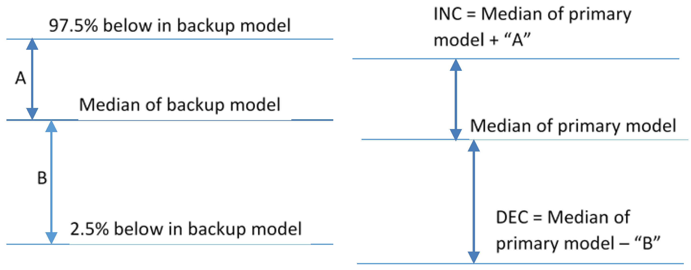
This procedure is represented in Figure 5. On the left of the graphic in Figure 5, “A”, for a given IV state, is the difference between the backup model median prediction for that IV state and the 97.5th percentile for the give IV state. “B” is the difference between the backup model median prediction and the 2.5th percentile. On the right hand side of the graphic, the INC prediction for a given IV state is the median prediction from the primary RA Model plus “A” and the DEC prediction for the same IV state is the primary RA Model median prediction less “B”.

The resulting model from this procedure will simply be called the “RA Model” for the remainder of the section.

4.2. Metrics for Comparing INC and DEC Predictions Efficacy

The Industry Model is compared to the RA Model using four metrics the CAISO [9] uses to assess the efficacy of the Industry Model predictions of the FRST INC and DEC requirement. These four metrics are calculated and compared between the Industry Model and the RA Model. The four metrics are:

Average Requirement—The average INC requirement and average DEC requirement in MW over all observations in a given fold. Computed the same for the Industry Model and the RA Model. The higher the average requirement, the higher the cost of maintaining enough capacity to access the market. The equation for this metric is as follows:

$$\mathrm{Average} \mathrm{INC} \mathrm{Requirement}=\frac{1}{\mathrm{n}}{{\displaystyle \sum }}_{\mathrm{j}}{\mathrm{INC} \mathrm{Requirement}}_{\mathrm{j}}$$

$$\mathrm{Average} \mathrm{DEC} \mathrm{Requirement}=\frac{1}{\mathrm{n}}{{\displaystyle \sum }}_{\mathrm{j}}{\mathrm{DEC} \mathrm{Requirement}}_{\mathrm{j}}$$

where j is a given observation, n is the total number of observations in each fold (34,435).

Coverage—A measure of (the inverse of) error. Measured as the percentage of time that the observed net load imbalance falls within the model-produced INC and DEC requirement. The lower the coverage, the higher the frequency that the net load imbalance falls outside the INC and DEC requirement. The thresholds are set at 2.5% and 97.5% based on historical data, so the coverage aims at 95% or an error of 5%, but when applied to unseen data, the Industry Model is actually in error 7% of the time.

Closeness—The average difference in MW between the observed net load imbalance and the model-produced requirement when the observed net load imbalance falls either inside or outside the INC or DEC requirement. If the observed net load imbalance is positive, it is measured against the INC requirement; if negative, it is measured against the DEC requirement. This metric measures how much the model is either over-estimating or under-estimating the capacity need, so the metric is actually an inverse of closeness. In this way, the metric can be thought of as Exceedance plus lost opportunity cost. The Closeness metric is reported separately for the INC and DEC requirements.

Exceedance—The average difference in MW between the observed net load imbalance and the model-produced requirement only when the observed net load imbalance falls outside the requirement, i.e., how much is the model under-estimating the need. The higher the exceedance value, the larger the gap between the INC or DEC capacity a participant contributed and what they actually needed, which can result in reliability issues if other market participants do not have unused capacity bid into the market. The Exceedance metric is also reported separately for the INC and DEC requirements.

For these metrics, one wants Average Requirement to be low, Coverage to be high, Closeness to be low, and Exceedance to be low.

To illustrate these metrics, Figure 6 provides 16 hypothetical examples of the INC and DEC requirements for the same time period of the RA Model and Industry Model, using the same 2.5%/97.5% thresholds, and of the (hypothetically) observed net load imbalance (the DV) for this time period. Each time period represents a different IV state for the RA Model and different historical data for the Industry Model; both the RA Model and the Industry Model thus have different INC and DEC requirements in different time periods.

For example, in Figure 6, the Average Requirement metric for INC reserves is computed by taking the average of all the light blue bars for the RA Model and the average of all the light orange bars for the Industry Model.

Table 11. Observed Net Load Imbalance and RA and Industry Model INC and DEC predictions for each interval from Figure 6.

		Observation Number from Figure 6
		1	2	3	4	5	6	7	8
1	RA Model INC	187 MW	295 MW	118 MW	396 MW	275 MW	182 MW	593 MW	258 MW
2	Observed Net Load Imbalance	171 MW	363 MW	−57 MW	106 MW	65 MW	−422 MW	425 MW	−132 MW
3	RA Model DEC	−318 MW	−472 MW	−276 MW	−165 MW	−124 MW	−586 MW	−324 MW	−388 MW
4	Industry Model INC	310 MW	242 MW	152 MW	323 MW	120 MW	253 MW	192 MW	232 MW
5	Observed Net Load Imbalance	171 MW	363 MW	−57 MW	106 MW	65 MW	−422 MW	425 MW	−132 MW
6	Industry Model DEC	−608 MW	−581 MW	−286 MW	−115 MW	−316 MW	−278 MW	−333 MW	−356 MW
		9	10	11	12	13	14	15	16
7	RA Model INC	326 MW	423 MW	51 MW	125 MW	166 MW	93 MW	104 MW	188 MW
8	Observed Net Load Imbalance	91 MW	193 MW	−384 MW	59 MW	−16 MW	143 MW	−139 MW	−95 MW
9	RA Model DEC	−185 MW	−90 MW	−340 MW	−171 MW	−108 MW	−130 MW	−341 MW	−579 MW
10	Industry Model INC	268 MW	434 MW	192 MW	101 MW	493 MW	261 MW	421 MW	197 MW
11	Observed Net Load Imbalance	91 MW	193 MW	−384 MW	59 MW	−16 MW	143 MW	−139 MW	−95 MW

shows the data from Figure 6 in tabular form for ease of review. Where bolded, the RA or Industry Model INC or DEC prediction is less than actual Observed Net Load Imbalance which results in an error and therefore a reduction in the Coverage metric. When not bolded, the RA or Industry Model INC or DEC prediction is greater than actual Observed Net Load Imbalance meaning the INC or DEC capacity requirement was sufficient to meet the Observed Net Load Imbalance in that interval. Note that Figure 6 and the accompanying Table 11 are illustrative, and do not show the advantages of the RA Model over the Industry Model; these advantages are clearly shown the Section titled “Industry Model and RA Model INC and DEC Prediction Results.”

The Coverage metric is computed by summing the number of times the observed net load imbalance falls within the INC and DEC range over all time periods. Time period 7, in Figure 6 or Table 11, shows where the RA Model has Coverage and the Industry Model does not as the observed net load imbalance is within the RA INC Requirement but greater than the Industry Model INC requirement. For the 16 time periods in the figure, the RA Model has Coverage in 13 time periods, while the Industry Model has Coverage in 12 periods.

The Closeness metric for INC reserves is computed as the difference between the observed net load imbalance and the INC requirement when the observed net load imbalance is positive, and the average over all time periods. The Closeness metric is the same for DEC except it’s applied against the DEC requirement when the observed net load imbalance is negative. Time period 14 in Figure 6 or Table 11 provides an example where the RA INC Closeness is slightly better than the Industry Model INC Closeness. However, this highlights the fact that Coverage is more important than Closeness because in this example even though the RA Model INC requirement is closer to the observed net load imbalance, the RA Model is in error whereas the Industry Model is not.

The Exceedance metric is the average difference between observed net load imbalance and the INC requirement when the observed net load imbalance is greater than the INC requirement. The same is computed for DEC when the observed net load imbalance is less than the DEC requirement. Time period 2, in Figure 6 or Table 11, shows an example where both the observed net load imbalance exceeds the RA Model INC requirement and the BN Model INC requirement but it is exceeded more for the Industry Model than the RA Model.

Table 12. Calculated metrics from Figure 6 example.

	Industry Model			RA Model			Delta RA Less Industry
	INC	DEC	Total	INC	DEC	Total	INC	DEC	Total
Avg. Requirement	261.9	357.1	619.1	236.2	287.3	523.5	(25.7)	(69.8)	(95.6)
Coverage	87.5%	87.5%	75.0%	87.5%	93.8%	81.3%	0.0%	6.3%	6.3%
Closeness	149.2	228.8	N/A	148.1	208.9	N/A	(1.1)	(19.8)	N/A
Exceedance	177.1	75.9	N/A	59.3	43.3	N/A	(117.9)	(32.6)	N/A

shows summary statistics for the four metrics computed based on the 16 samples from Figure 6. For these metrics, one wants Average Requirement to be low, Coverage to be high, Closeness to be low, and Exceedance to be low.

4.3. Industry Model and RA Model INC and DEC Predictions Results

A test was performed on the RA Model to compare the prediction efficacy to that of the Industry Model. The Average Requirement, Coverage, Closeness, and Exceedance metrics are reported for the Industry Model and the RA Model and the delta between them.

The test scaled the RA Model upper and lower threshold percentiles so that the RA INC and DEC produced the exact same Coverage between the two models. For example, referring to Figure 6, this would have meant scaling the RA upper and lower thresholds so that of the 16 observations, there were the exact same number of INC errors and DEC errors between the Industry Model and the RA Model: when the observed net load imbalance was positive, it fell outside the INC requirement the same number of times in both the Industry Model and the RA Model, and when the observed net load balance was negative, it fell outside the DEC requirement the same number of times in both the Industry Model and the RA Model. This test is intended to see if after fixing Coverage of the RA Model to be identical to the Industry Model the Average Requirement, Closeness and Exceedance metrics are reduced under the RA Model relative to the Industry Model.

Reduction in all three other metrics for the RA Model is indeed found.

Table 13. Test Results.

	Industry Model			RA Model			Delta RA Less Industry
	INC	DEC	Total	INC	DEC	Total	INC	DEC	Total
Avg. Requirement	272.8	322.4	595.3	210.1	234.3	444.3	(62.7)	(88.2)	(150.9)
Coverage	95.4%	97.6%	93.0%	95.4%	97.6%	93.0%	0.0%	0.0%	0.0%
Closeness	190.2	249.1	N/A	153.1	200.3	N/A	(37.1)	(48.8)	N/A
Exceedance	99.6	121.3	N/A	92.4	109.0	N/A	(7.1)	(12.3)	N/A

shows the resulting statistics. As can be seen in Table 13, while Coverage is held the same for the Industry and RA Model, the Average Requirement, Closeness and Exceedance are all reduced relative to the Industry Model. This test shows that if the Industry Model Coverage (error rate) is acceptable, because the RA Model makes a more accurate prediction of the upper and lower INC and DEC thresholds, the Average Requirement for INC and DECs can be reduced. On average, 62.7 MW less INC, 88.2 MW less DEC, and 150.9 MW less total capacity would have to be held, while still maintaining the same Coverage. Further, Exceedance is also lower, 7.1 MW lower for INC, 12.3 MW lower for DEC. Even though Coverage is the same as the Industry Model, when the observed net load imbalance exceeds the RA Model INC or DEC requirement, it exceeds by less, on average, than the Industry Model.

Figure 7 shows more detail about the results of Test 1 and the Exceedance metric. Given the same 93% Coverage (7% error) for the RA and Industry Model, when the RA Model (blue bars) is in error, the error is smaller than the Industry Model.

4.4. RA Backup Model INC and DEC Prediction Results

The RA backup model was also tested by itself to show that the point estimate and using the RA INC and DEC prediction procedure is superior to using the backup model by itself. The model was tested on BCD training data and A test data. The backup model performed better than the Industry Model on the single point prediction, but worse than the RA Model in terms of R squared, MAE, and MSE, as expected.

Table 14. RA Backup Model Point Estimate Summary Statistics.

	Industry Model	RA Model	Backup RA Model
R squared	7.5%	34.1%	15.0%
MAE	121.7	86.8	102.4
MSE	27,339.7	16,616.8	21,409.9

shows a comparison of the resulting summary statistics. On this fifth fold, the RA Backup Model also performed better on R squared, MAE, and MSE than the BN model and all SVR models, but not as well as the MLP model.

The backup model was also assessed for its ability to predict INC and DEC capacity using the same test previously applied to the RA Model. The test held Coverage equal to the Industry Model to see if the Average Requirement was reduced.

Table 15. RA Backup Model INC and DEC Predictions Compared to RA Model.

	Increase in Avg. Requirement
Total Avg.	64.8
INC Avg.	30.3
DEC Avg.	34.5

shows how the backup model performed relative to the RA Model. The three numbers shown are deltas from the best RA Model. For the same Coverage, the backup model required 64.8 MW more Total capacity than the RA Model. This comparison shows that the backup model (where INC and DEC are applied to the backup model point prediction) did not perform as well as the Best RA Model (where the INC and DEC of the backup model are applied to the Best RA Model point prediction).

5. Discussion

The RA method performed better than the other machine learning methods applied in this research when comparing single point estimate predictions for a given observation (section titled “Results of DV prediction: comparing ML methods to Industry Model”). Our presumption is that RA performed better than the other methods because it is able to efficiently determine the optimal set of IVs to be used in the model whereas MLP and SVR used f-regression to select the predictive IVs, and the BN algorithm is limited in network complexity by the computational cost of the EM algorithm to make predictions about missing values or missing states. Although we did not perform a hyper-parameter exploration for SVR and NN as that would have been an entire study of its own, it was not warranted for the actual purpose of the first part of the study which was to use point estimate prediction success to select a machine learning method to model INC and DEC predictions in the second part of the study. Our use of RA and BN was similar in that we used the simplest form of RA and did not perform any preprocessing for RA or BN. Thus all four ML methods did not utilize an elaborate pre-processing and were thus treated equally.

The best RA Model resulted in 15 of the 22 possible IVs being included in the model. Of these, the most predictive variables are hour of day (HourofDayx2hrxgroups), the 48 h wind forecast (VERFCFHFrtegt), and Sunrise/Sunset (SunriseSunset) found in Table 7. These variables were also found and included in the best SVM and MLP models. The Sunrise/Sunset IV is a time based IV that reflects 5 a.m.–7 a.m. PST and 5 p.m.–7 p.m. PST. It is a simple variable that was intended to capture some of the morning and evening solar and load ramp uncertainty.

Similar to the Sunrise/Sunset variable, the 48 h wind forecast variable reflects times of energy imbalance uncertainty. Its information content is useful since knowing the wind forecast provides information about the maximum amount of INC that could be needed and maximum amount of DEC that could be needed. Additionally, the relationship between wind power output and wind speed shown in Figure 8 illustrates why the wind forecast is an important predictive variable. The greatest uncertainty in wind power output is when the wind forecast is in the middle of the nameplate (total possible output) of a plant. At low and high wind power output, the output changes little for small changes in wind speed, whereas at medium output, the output changes more significantly for the same small change in wind speed. Thus, actual wind power output is more variable when forecast output is around half of the plant nameplate. The RA Model is improved relative to the Industry Model by encompassing the wind forecast. The CAISO has been considering adjusting its methodology to account for the wind forecast, and the RA Model results and empirical results suggest that the predictive information contained in the wind forecast has the potential to significantly improve INC and DEC predictions.

Additionally, interesting, the best RA Model, and each best model from all 5 folds shown in Table 6 included the 48 h wind forecast, 96 h wind forecast and 120 h wind forecast. This is an indication that there is additional, significant information, contained in the 96 and 120 h wind forecasts not contained in the 48 h wind forecast. This is supported by work previously done at Bonneville Power Administration. This work found that larger differences in wind power output forecasts of different time durations result in increased uncertainty in actual wind power output, while smaller differences in wind power output forecasts of different time durations result in reduced uncertainty in actual wind power output. Our presumption is that the differences between forecasts of wind power output of different time durations is a result of greater or less uncertainty in the weather pattern. While the CAISO has considered adjusting their model to account for the wind forecast, this research suggests that including the closest-in wind forecast is useful and also including forecasts of longer time durations could further improve the prediction results.

Last, it was surprising that each of the best fold models from Table 6 contained an RTD variable, Load variable and FMM variable but never two of the same type of variables in a single model. For example, the best Fold 1 model contained NLMinRTD and Fold 2 contained NetLoad RTD, which are related but different IVs, but no best fold model included both of these Net Load variables, nor both Load or FMM variables.

6. Conclusions

The primary aim of this research was to build an INC and DEC capacity prediction model that improves upon the current Industry Model. The results in this paper (section titled “Results of INC/DEC prediction: comparing RA Model to Industry Model”) show that the best RA Model does in fact do that. As shown in the test results, the best RA Model reduces Total reserves relative to the Industry Model by 150.9 MW on average, a reduction of 25.4%; INC reserves are reduced on average 62.7 MW, a reduction of 23.0% relative to the Industry Model, while DEC reserves are reduced on average 88.2 MW, a reduction of 27.3. Additionally, Closeness and Exceedance metrics are also reduced significantly relative to the Industry Model. Conservatively, reducing the reserve requirement by this amount would result in approximately $4 million (INC savings would be $168/MW-day × 365 days × 62.7 MW = $3.84 million. DEC savings would be $12/MW-day × 365 days × 88.2 MW = $386 thousand) in annual savings for the Bonneville Power Administration which is one of nineteen WEIM participants and which is the focus of the data analysis in this paper.

This paper also discusses the results and theoretical comparisons between RA and BN as they are both machine learning methods that are analytically very similar. This research built on prior work [28] and used a concrete example to show that the best RA Model identified in this research can be replicated exactly in a BN. However, the BN search algorithm, in particular the computational cost of the EM algorithm, prevent such complex BN models from being found by standard BN search algorithms. Further, this research (Figure 4) used toy examples to show that several BNs with different edge topologies are analytically equivalent to a single RA graph, these toy examples further amplify and illustrate prior work [28].

Another aim of this research was to identify predictive variables of net load imbalance. This research also accomplishes this aim showing that wind forecast, sunrise/sunset, and hour of day are primary predictors of net load imbalance and should be considered for inclusion in any future industry application.

Logical extensions of the methods comparison could test other pre-processing steps and hyper-parameter exploration for MLP and SVR such as z-score [45], clustering evaluation criteria [45,46] and other techniques [47,48,49] or using the IVs determined by the best RA model as the IVs used in MLP and SVR. Additionally, other ML methods could be tested for prediction efficacy. Additionally, the use of more complex RA models, such as models with loops and state-based models, could be investigated. Prior research on electricity data has shown that different ML methods have certain advantages and disadvantages given the particular application. [8]. Further extensions could also refine the Sunrise/Sunset variable to capture the optimal Sunrise/Sunset timeframe for each WEIM participant where solar penetration is the highest, or more acutely a focus on the window of time of peak net load ramp or decline.