Genetically Optimized Extended Kalman Filter for State of Health Estimation Based on Li-Ion Batteries Parameters

Abstract

The state of health (SOH) is among the most important parameters to be monitored in lithium-ion batteries (LIB) because it is used to know the residual functionality in any condition of aging. The paper focuses on the application of the extended Kalman filter (EKF) for the identification of the parameters of a cell model, which are required for the correct estimation of the SOH of the cell. This article proposes a methodology for tuning the covariance matrices of the EKF by using an optimization process based on genetic algorithms (GA). GAs are able to solve the minimization problems for the non-linear functions, and they are better than other optimization algorithms such as gradient descent to avoid the local minimum. To validate the proposed method, the cell parameters obtained from the EKF are compared with a reference model, in which the parameters have been determined with proven procedures. This comparison is carried out with different cells and in the whole range of the cell’s SOH, with the aim of demonstrating that a single tuning procedure, based on the proposed GA process, is able to guarantee good accuracy in the estimation of the cell parameters at all stages of the cell’s life.

1. Introduction

In countless applications of lithium batteries, the real cycling and environmental conditions affect cells degradation. Nowadays, there is a worldwide spreading of applications, powered by Li-Ion batteries. A non-exhaustive list includes: home appliances such as vacuum cleaners and kitchen tools, personal mobility vehicles such as scooters and e-bikes, and professional tools for gardening, agriculture and the industrial sector. In most applications, the battery management system (BMS) also includes algorithms for the battery state estimation, such as state of charge (SOC), state of health (SOH) and state of safety (SOS) [1]. Proper SOC estimation allows power delivery optimization and improves the user experience, while a SOH estimation gives an indication of the residual functionality or residual value of the battery. SOH estimation should be performed regardless of the cell’s past life and of the degradation processes that have occurred [2]. For this purpose, the use of life models based on pre-calculated data [3] are often unreliable.

The Kalman filter (KF), in all its forms, is an excellent method for determining the states of the cell. This method has good accuracy and reliability, even compared to other methods [4], such as the particle filter [5]. For this reason, in the literature, there are many examples of the application of KF algorithms for SOC estimation [6,7,8]. SOH cannot be estimated directly using the KF, but it can be obtained through precise estimation of cell parameters, such as internal cell resistance and capacitance [9,10,11,12,13]. In the literature, where more filters are often used simultaneously, the most popular method is that explained by [4], which uses the dual extended Kalman filter. A variation of this method is presented in [13], their proposed method is called dual fractional order extended Kalman filter. Other authors propose different filters used together with [10] that combines the use of the H-infinite filter for the estimation of SOC and the unscented Kalman filter (UKF) for the estimation of cell parameters.

The KF has been proposed for the search of the model parameters’ values, and in particular for internal cell resistance $R_0$ by some authors such as [14]. Unfortunately, the performance of these KFs is strictly dependent on the proper choice of coefficients of the covariance matrices, which must be carefully chosen for each cell type and chemistry. Often, in the literature, the methodology for determining the coefficients of the covariance matrices are not shown, so the idea is to present an automated procedure for tuning these matrices. The proposed method, called generically genetically optimized extended Kalman filter (GO-EKF) is a procedure that combines an extended Kalman filter (EKF) implementation with a genetic algorithm. The search procedure, which must be carried out once per cell type, finds optimal and reliable coefficients for the covariance matrices that will be used by the EKF in any aging condition of the cell. To validate the proposed method, a reference model is used for comparing the results of the EKF. The adopted reference model [3] is based on a “single polarization” structure and relies on a widely accepted methodology for determining the parameters from experimental tests. The reference model is adopted to provide true values of internal resistance under any condition of SOC and SOH; on the other hand, real cell tests are used to evaluate the performance of the proposed EKF in estimating the cell voltage. It is possible to estimate the SOH based on the internal resistance, using known methods such as [11,15]. This paper proposes and validates an optimization methodology, which is able to correctly estimate the internal resistance of the cell $R_0$ and its voltage. Furthermore, it makes available all the necessary information to be used in future implementations for SOH estimation.

Section 2 describes the details of the reference model, the parameter estimation method and the accuracy of the reference model, by comparing its results with the experimental data. Section 3 briefly describes the EKF applied to the modeling of a Li-Ion battery, giving an overview of the results obtained by other authors, the tuning methods and the covariance matrices coefficients they used. This section introduces the proposed EKF implementation, giving the chosen state variables and the details of transition, measurements and covariance matrices. At the end of section, the optimization process for the covariance matrices based on the proposed genetic algorithm is presented. The main goal of the proposed approach is to speed up the tuning process, with no need for performing specific tests. Section 4 hosts the final tests results, and claims the performance of the proposed GA-optimized EKF in the estimation of cell voltage and resistance.

2. Reference Model

For evaluating the performance of the proposed EKF, with automated covariance matrix calculation, a widely used equivalent circuit model (ECM) is considered as a reference cell model. The reference model’s tuned parameters are used as reference values, to be compared with the EKF outputs. Among the model’s parameters, the $R_0$ value is used as reference parameter. The reason behind this choice is the impossibility to directly measure the $R_0$ during cell operation with real current profiles. The accuracy of the EKF will be validated by comparing its output with the measured output voltage and the other ECM parameters calculated with specific pulse tests.

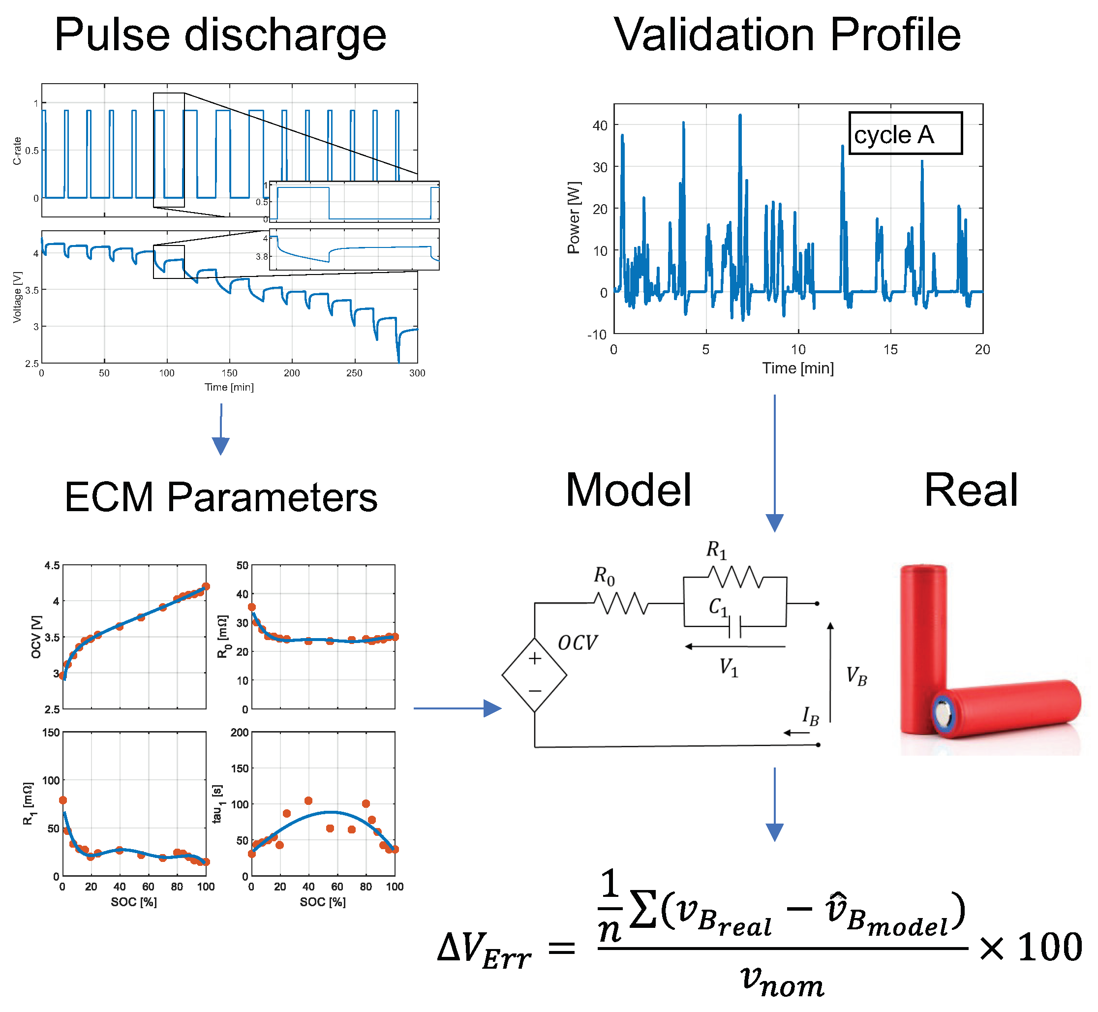
2.1. Model Description

Among the ECMs, the single polarization (SP) type is commonly chosen as it provides good accuracy despite the small amount of required parameters. In fact, only five parameters, namely the open circuit voltage: $OCV$, the series resistance: $R_0$, the R/C branch: $R_1$, ${\tau }_1$ and the voltage on the capacitor: $V_c$ are required. This makes the tuning process easier. All the mentioned parameters are $SOC$-dependent.

In order to determine the model parameters, a specific discharge test called “pulse discharge” is used. The voltage measurement performed on the actual cell during the test allows us to compute the model parameters. This procedure is thoroughly described in [16,17,18,19]. With the pulse discharge test, only a few values are available; therefore, an interpolating function was used to make all the parameters continuous as a function of the SOC.

$$\begin{array}{c}\hfill \begin{array}{c}\hfill v_{B_k}=OCV\left(SO{C}_k\right)-R_0\left(SO{C}_k\right)\times i_{B_k}-V_{c_k}\end{array}\end{array}$$

(1)

$$\begin{array}{c}\hfill \begin{array}{c}\hfill V_{c_K}=(1-\frac{dt}{{\tau }_1\left(SO{C}_k\right)})V_{c_{K-1}}+\\ \hfill +\frac{dt}{{\tau }_1\left(SO{C}_k\right)}\times R_1\left(SO{C}_k\right)\times i_{B_k}\end{array}\end{array}$$

(2)

$$\begin{array}{c}\hfill \begin{array}{c}\hfill SO{C}_k=SO{C}_{k-1}-\frac{i_{B_k}\times dt}{C_{nom}}\end{array}\end{array}$$

(3)

The set of interpolation functions, representing the SP model, written in discrete form for the sample period dt, is shown above in Equations (1)–(3). Equation (2) are obtained using the first order Taylor approximation. To calculate the state of charge, Coulomb counting was used. All the parameters of these interpolation functions have been obtained using the search methodology described in [16].

$$\begin{array}{c}\hfill V_{Err}=\frac{\frac{1}{n}\sum |{\widehat{v}}_{B_{model}}-v_{B_{real}}|}{v_{nom}}\times 100\end{array}$$

(4)

2.2. Model Tuning and Validation

Figure 1 shows a scheme for the tuning and validation of the reference model. In particular, the process consists of two phases: Firstly, the cell model parameters are estimated with a pulse discharge test. Afterwards, the model is validated with cycle A. We chose to validate the model on this profile because it will be used later as a reference to test the algorithm. The equipment used for both pulse discharge and cycling is shown in Figure 2 and its specifications are briefly listed in

Table 1. Test bench equipment specifications.

Power Supply	TDK-Lambda GEN60-40
Electronic Load	BK Precision 8514
Wattmeter	Yokogawa WT310EH
Cryostat	Jeio Tech RW3-0525P
Controller	NI cRIO-9066

. All the tests are performed in a controlled-temperature room in order to minimize any effect of the temperature on the cell parameters.

As previously introduced, this research relies on a dependable reference model for providing the accurate estimation of the $R_0$ resistance, to be used in any condition for evaluating the EKF performance.

2.2.1. Tuning of Model Parameters

In the tuning phase, data obtained from a pulse discharge test, performed on an actual cell, are used for determining the cell model parameters $OCV$, $R_0$, $R_1$, and ${\tau }_1$, as described in [16].

Three “21.700” cell specimens, from different manufacturers, have been used for this research (see pictures of Figure 3). The cells have been sampled at different life cycle conditions, ranging from new cells to aged cells.

Table 2. Average output voltage error of the reference model.

Test	Cell Name	Cycle Number	Avg Verr [%]
1“Cycle A”	LG“INR2170050T”	1	0.94
2“Cycle A”	LG“INR2170050T”	100 ${}^{\mathrm{a}}$	0.59
3“Cycle A”	LG“INR2170050T”	200 ${}^{\mathrm{a}}$	0.40
4“Cycle A”	SAMSUNG“INR2170050E”	1	0.76
5“Cycle A”	SAMSUNG“INR2170050E”	100 ${}^{\mathrm{a}}$	0.97
5“Cycle A”	SAMSUNG“INR2170050E”	300 ${}^{\mathrm{a}}$	0.84
6“Cycle A”	SAMSUNG“INR2170050E”	500 ${}^{\mathrm{a}}$	1.04
7“Cycle A”	MOLICEL“INR21700P42A”	1	0.83

^a Discharge CC 1 C Cut-Off 2.5 V, 25 °C; charge: CC-CV at 0.5 C 4.2 V, 50 mA, 25 °C.

shows the cycle number of each tested sample. All the parameters are evaluated at correspondent cycles.

2.2.2. Model Validation

For the validation phase, an arbitrary cycle is applied on the actual cell. In more detail, the profile used is obtained from a standardized driving cycle for passenger cars (WLTC). As the driving cycle is defined as a speed profile, the reference power is calculated by introducing the vehicle model [20]. In other words, the validation cycle represents the hypothetical operation of the cell in an automotive application. The reference power profile has been applied to the cell model as well, as it returns the modeled voltage profile to be compared with the test results. The tests begin with fully charged cells, and stop when the discharge cut-off voltage is reached. Using the same testing equipment of Table 2, all the selected cells at the different aging conditions have been tested with the power profile. The average error between the terminal voltage $V_{B_{real}}$, measured on the actual cell, and the modeled voltage ${\widehat{V}}_{B_{model}}$ was therefore calculated. Table 2 reports the average errors computed with the Equation (4).

3. KF and EKF for Cell Parameter Identification

This paper focuses on the use of the Kalman filter for the estimation of Li-Ion cells parameters. For the determination of the coefficients of the covariance matrices, a heuristic optimization algorithm is proposed, in particular a genetic algorithm.

With this approach, it is possible to determine the best set of elements values for the covariance matrices in order to minimize the error in the estimation of the cell voltage.

3.1. Kalman Filter

The Kalman filter [21] recursively calculates an estimated state of a linear dynamic system as the weighted average between the predicted state and the measured state determined from the available measurements. KF relies on the state-space formulation of linear dynamic systems in the discrete time domain. Assuming discrete time sample $\mathit{k}$, the state vector ${\mathit{x}}_k$ contains the minimal data set required to predict the future k + 1 behavior of the system by using data taken from the past step $\mathit{k}$. Referring to state-space linear system representation, the transition matrix ${\mathbf{F}}_k$ brings the state from instant $\mathit{k}$ to the future state $\mathit{k}+\mathit{1}$, and matrix ${\mathbf{B}}_k$ represents the effect of a set of input variables ${\mathit{u}}_k$ to the future state ${\mathit{x}}_{k+1}$. Assuming the vector ${\mathit{y}}_k$ as the set of output measurable quantities, the measurement matrix ${\mathbf{H}}_k$ determines the output from the states. The straightforward matrix ${\mathbf{D}}_k$ directly influences the output ${\mathit{y}}_k$ with the input variables ${\mathit{u}}_k$.

If the analyzed system is non-linear, it is possible to extend the use of Kalman filtering through a linearization procedure. The resulting filter is referred to as the extended Kalman filter (EKF) [22]. The non-linear system is still described by the state-space model representation, following the KF basic description. In EKF, $\mathit{f}({\mathit{x}}_k,{\mathit{u}}_k)$ and $\mathit{h}({\mathit{x}}_k,{\mathit{u}}_k)$ represent the non-linear transition matrix and the non-linear measurement matrix, respectively.

The basic principle of the extended Kalman filter consists in linearizing the system equations at each time instant. The linearization process requires us to calculate the partial derivatives of the two functions f and g with respect to each of the estimated states ${\widehat{\mathit{x}}}_k$ and ${\widehat{\mathit{x}}}_k^{-}$, for obtaining the new transition matrix ${\mathbf{F}}_k$ and the new measurement matrix ${\mathbf{H}}_k$:

Both updated state ${\widehat{\mathit{x}}}_k$ and updated covariance ${\mathbf{P}}_k$ will be used in the following time interval $k+1$ for the prediction step. All the expressions used in the EKF implementation are given in Algorithm 1, following a common notation, as introduced by [23].

Algorithm 1: Summary of non-linear extended Kalman filter equation.

Non-linear state-space model ${}^{\mathrm{a}}$             ${\mathit{x}}_{k+1}=\mathit{f}({\mathit{x}}_k,{\mathit{u}}_k)+{\mathit{w}}_k$          $\mathbb{E}=\left[w_n{w_k}^T\right]=\left\{\begin{array}{cc}{\mathbf{Q}}_k& n=k\\ 0& n\ne k\end{array}\right.$             ${\mathit{y}}_k=\mathit{h}({\mathit{x}}_k,{\mathit{u}}_k)+{\mathit{v}}_k$          $\mathbb{E}=\left[v_n{v_k}^T\right]=\left\{\begin{array}{cc}{\mathbf{R}}_k& n=k\\ 0& n\ne k\end{array}\right.$     Definitions             ${\mathbf{F}}_k=\frac{\partial \mathit{f}({\mathit{x}}_k,{\mathit{u}}_k)}{\partial \mathit{x}}{|}_{\mathit{x}={\widehat{\mathit{x}}}_k}$             ${\mathbf{H}}_k=\frac{\partial \mathit{h}({\mathit{x}}_k,{\mathit{u}}_k)}{\partial \mathit{x}}{|}_{\mathit{x}={\widehat{\mathit{x}}}_k^{-}}$     1. Initialization          For $k=0$, set                 ${\widehat{\mathit{x}}}_0=\mathbb{E}\left[{\mathit{x}}_0\right]$,             ${\mathbf{P}}_0=\mathbb{E}\left[({\mathit{x}}_0-{\widehat{\mathit{x}}}_0){({\mathit{x}}_0-{\widehat{\mathit{x}}}_0)}^T\right]$     2. Computation          For k = 1, 2, …, compute          2.1 Time Update                State Estimate: ${\widehat{\mathit{x}}}_k^{-}=\mathit{f}({\mathit{x}}_{k-1},{\mathit{u}}_{k-1})$                Error covariance: ${\mathbf{P}}_k^{-}={\mathbf{F}}_{k-1}{\mathbf{P}}_{k-1}{\mathbf{F}}_{k-1}^T+\mathbf{Q}$          2.2 Measurement update                Kalman gain: ${\mathbf{G}}_k={\mathbf{P}}_k^{-}{\mathbf{H}}_k^T{[{\mathbf{H}}_k{\mathbf{P}}_k^{-}{\mathbf{H}}_k^T+{\mathbf{R}}_k]}^{-1}$                Output evaluation: ${\widehat{\mathit{y}}}_k={\mathbf{H}}_k{\widehat{\mathit{x}}}_k^{-}+{\mathbf{D}}_k{\mathit{u}}_k$                State estimation: ${\widehat{\mathit{x}}}_k={\widehat{\mathit{x}}}_k^{-}+{\mathbf{G}}_k[{\mathit{y}}_k-{\widehat{\mathit{y}}}_k]$                Error covariance: ${\mathbf{P}}_k=(\mathbf{I}-{\mathbf{G}}_k{\mathbf{H}}_k){\mathbf{P}}_k^{-}$     ${}^{\mathrm{a}}$ ${\mathit{w}}_k$ and ${\mathit{v}}_k$ are independent, zero-mean Gaussian noise process of covariance matrices $\mathbf{Q}$$\in {\mathbb{R}}^{n\times n}$ and $\mathbf{R}$$\in {\mathbb{R}}^{m\times m}$, respectively [21]. ${\mathit{x}}_k\in {\mathbb{R}}^n,{\mathit{y}}_k\in {\mathbb{R}}^m,{\mathit{u}}_k\in {\mathbb{R}}^l$.     ${\mathbf{F}}_k\in {\mathbb{R}}^{n\times n},$     ${\mathbf{B}}_k\in {\mathbb{R}}^{n\times l},{\mathbf{H}}_k\in {\mathbb{R}}^{m\times n},{\mathbf{D}}_k\in {\mathbb{R}}^{m\times l}$.

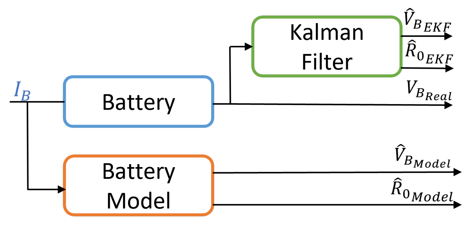
3.2. Extended Kalman Filter Applied to the Cell Parameters Estimations

Table 3. Summary of EKF literature applied to battery state estimation.

Filter Type	Model Type	State Variables	Covariances ${\mathit{Q}}_{\mathit{k}}$, ${\mathit{R}}_{\mathit{k}}$	Methodology	Voltage Error	Reference
AKF	Thevenin	$SOC$	[1] [1]	adaptive estimation	Max < 20% Avg N/A	[24]
EKF	RC model	[$V{c}_1$, $V{c}_2$, Vb, $1/C_1$]	$[0.5,0.5,0.005,{10}^{-4}]$ $\left[10\right]$	N/A	Max < 5% Avg N/A	[25]
EKF	RC model	[$V{c}_1$, $V{c}_2$, Vb, $1/C_1$]	$[0.005,0.07,0.9,$ 10−4][10]	N/A	Max < 4% Avg N/A	[26]
EKF	SP model	[SOC, $Vc$]	N/A	computed each iteration	Max < 5% Avg < 2%	[27]
EKF	SP model	[SOC, $Vc$]	$[0.25,0.25]$ $\left[0.01\right]$	N/A	Max < 10% Avg < 5%	[12]
EKF	SP model	[$SOC$, $Vc$]	$[0.005,0.4191,0.8143]$ $\left[2\right]$	[28]	Max < 2% Avg N/A	[29]
EKF	SP model	[$Vc$, $SOC$]	N/A	N/A	Max < 10% Avg 0.17%	[30]
DEKF	SP model	[$Vc$, $SOC$] [$R_0$, C, $R_1$, $C_1$]	$[{10}^{-9},{10}^{-15}]$ $[{10}^{-9},{10}^{-6},{10}^{-9},{10}^{-3}]$$[5\times {10}^{-7}]\left[0.0013\right]$	[31]	Max < 2% Avg N/A%	[4]
I EKF	SP model	$[SOC,V_c]$ $[R_0,R_1,C_p]$	$[0.01,-0.01]$ $\left[0.04\right]$ N/A	improve method [32]	Max < 1.4% Avg N/A%	[33]
EKF	DP model	$[V{c}_1,V{c}_2,Vb,1/R_1,$ $1/C_1,1/R_2,1/C_2]$	N/A	N/A	Max < 4.8% Avg 0.06%	[34]
ACKF	DP model	[$V{c}_1$, $V{c}_2$, $SOC$]	N/A	adaptive estimation	Max < 2.2% Avg N/A%	[35]
AEKF	DP model	[$V{c}_1$, $V{c}_2$, $SOC$]	$[{10}^{-3},{10}^{-3},{10}^{-3}]$ $[\mathrm{N}/\mathrm{A}]$	adaptive estimation	Max < 2.2% Avg N/A%	[34]
DEKF	DP model	$[Vc, SOC]$ $[R_0, C, R_1, C_1,$ R2, C2]	$[{10}^{-9},{10}^{-15}]$ $[{10}^{-9},{10}^{-6},{10}^{-9},{10}^{-3},$ 10−9, 10−3] [5 × 10−7][0.0013]	[31]	Max < 2% Avg N/A%	[4]
DEKF	DP model	$[Vc1,Vc2,SOC]$ $[R_0,C]$	N/A	N/A	Max < 1% Avg N/A%	[36]
DEKF	DP model	$[SOC,Vc1,Vc2]$ $[R_0,C]$	$[0.64,0.063,0.063]$ $[1.69\times {10}^{-4},5.67\times {10}^{-4}]$ $\left[0.77\right][7.27\times {10}^{-4}]$	numerical optimization	Max < 1% Avg N/A%	[37]

reports a list of relevant articles focusing on the application of the Kalman filter for the estimation of Li-Ion batteries parameters. The table shows the authors’ state space variable selection, the values of the covariance matrices, when available, and the performance of the method for the estimation of the cell voltage. The proposed model differs from those reported in Table 3 for the set of state variables used for the cell representation, which are derived from the SP model [12] shown in Figure 1 and listed hereinafter: the voltage of the RC branch $V_C$, the DC resistance $R_0$, the resistance of the RC branch $R_1$, and the time constant of the RC branch ${\tau }_1=R_1{C}_1$. These parameters have been chosen as state variables because of their high dependency on the cell aging. In accordance with all the implementations given in Table 3, the open circuit voltage $OCV$ is excluded from this list because of its limited dependency on the SOH. The OCV characteristics, if not provided, can easily be determined as a function of the SOC through simple tests and given either as a look-up table or a polynomial function of the SOC.

To summarize, the state variable vector $\mathit{x}$ is defined as:

$$\begin{array}{c}\hfill \mathit{x}=\left[\begin{array}{c}{V}_c\\ R_0\\ R_1\\ {\tau }_1\end{array}\right]\end{array}$$

(5)

The input variable vector u is defined by the cell current $i_B$ only:

$$\begin{array}{c}\hfill \mathit{u}=\mathit{u}=\left[i_B\right]\end{array}$$

(6)

In addition, the output variable vector y is defined by the cell voltage $v_B$ only:

$$\begin{array}{c}\hfill \mathit{y}=\mathit{y}=\left[v_B\right]\end{array}$$

(7)

The EKF estimator is implemented by using the notation and procedure introduced in Section 3.1 and the discretization time interval $\mathrm{\Delta }t$.

$$\begin{array}{c}\hfill \mathit{f}({\mathit{x}}_k,{\mathit{u}}_k)=\left[\begin{array}{c}{V}_{c_k}(1-\frac{\mathrm{\Delta }t}{{\tau }_{1_k}})+\frac{\mathrm{\Delta }t}{{\tau }_{1_k}}{R}_{1_k}{i}_{B_k}\\ R_{0_k}\\ R_{1_k}\\ {\tau }_{1_k}\end{array}\right]\end{array}$$

(8)

$$\begin{array}{c}\hfill \mathit{h}({\mathit{x}}_k,{\mathit{u}}_k)=[V_{O{C}_k}-V_{c_k}-R_{0_k}{i}_{B_k}]\end{array}$$

(9)

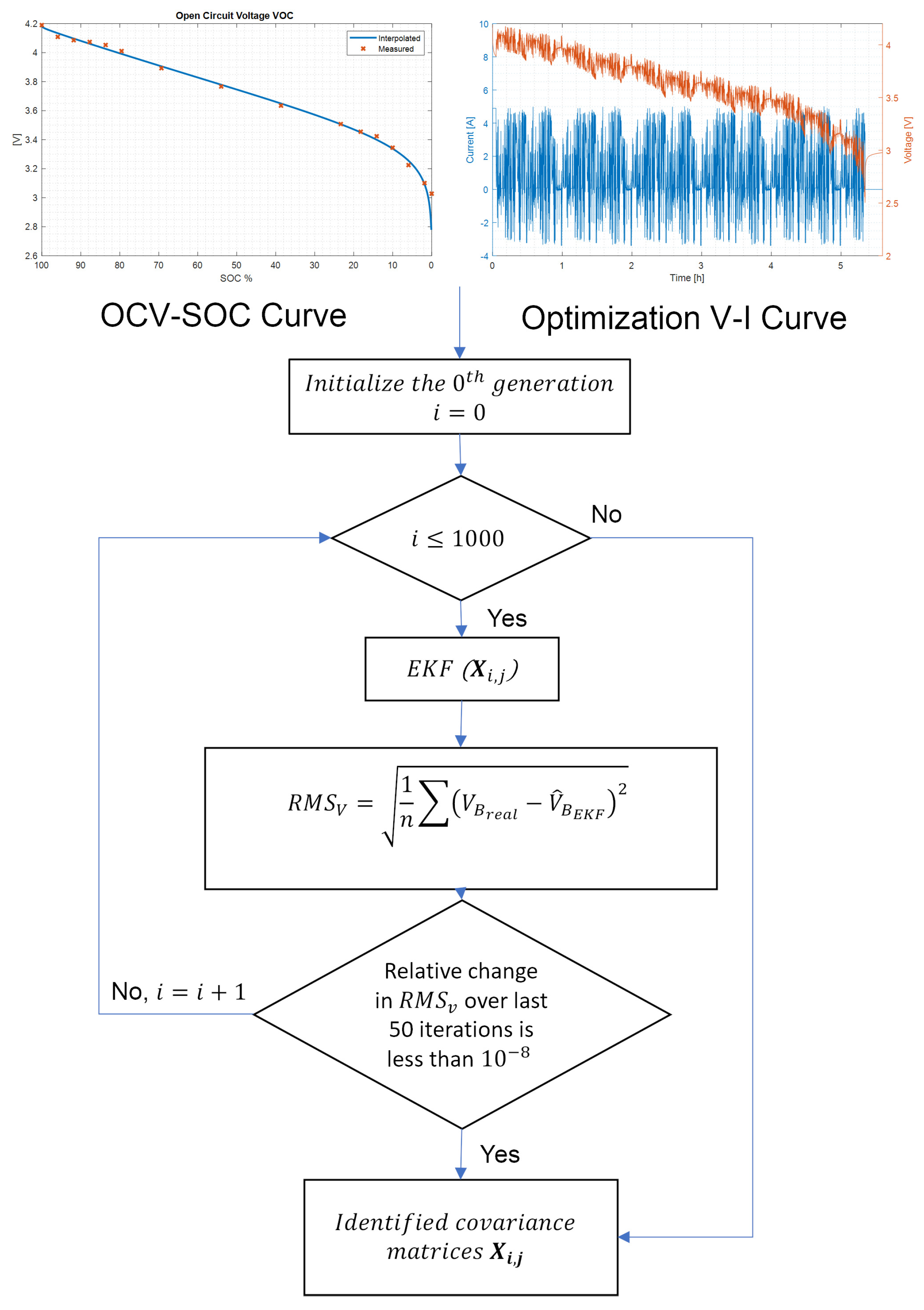
3.3. Genetic Algorithm for EKF Covariance Matrices

The proposed EKF relies on a method for determining the coefficients of the covariance matrices Q and R, using heuristic search based on a genetic algorithm. $\mathbf{Q}$$\in {\mathbb{R}}^{4\times 4}$ and $\mathbf{R}$$\in {\mathbb{R}}^{1\times 1}$ are diagonal matrices, with all and only the elements on the main diagonal different from zero.

All the procedures for the GA have been implemented following [38,39]. Evolutionary search is generally better than random search and is not susceptible to the hill-climbing behaviors of gradient-based search. No gradient information needs to be presented to the algorithm [39,40].

The genetic algorithm is embedded in an optimization session of the EKF introduced in Section 3.2. This session is fed by the cell measurements, obtained during the normal operation of the cell. The learning session finds the best fitting values for the coefficients of the two covariance matrices by minimizing the error in the output cell voltage estimated by the EKF. Using these automated procedures for tuning the coefficients of the covariance matrices, shown in Figure 4, a significant improvement in the accuracy of the cell parameter, estimated by the EKF, is expected. In the proposed genetic algorithm, a sample (or individual) ${\mathbf{X}}_{j,i}$ of the population is a vector whose elements (or genes) are the unknown coefficients to be inserted into the covariance matrices Q and R.

$$\begin{array}{c}\hfill {\mathbf{X}}_{j,i}=[Q_{{1,1}_{j,i}},Q_{{2,2}_{j,i}},Q_{{3,3}_{j,i}},Q_{{4,4}_{j,i}},R_{{1,1}_{j,i}}]\end{array}$$

(10)

where the index j represents the sample of the population (individual) in each i iteration (or generation). The proposed genetic algorithm selects the individual ${\mathbf{X}}_{j,i}$ with the best combination of genes through the procedure that is described step by step below. In the

Table 4. Parameters for setting the genetic algorithm.

Population m	20
Children l	4
Mutation Probability p	$50\%$
Mutation Range	${10}^4\to {10}^{-15}$
Fitness Target	${10}^{-8}$
Last Generation	1000

are summarized all the parameters used in the algorithm.

(1)

Initialization $i=0$

In the initial function, the number m of individuals of the population to observe is defined. At the initial step, the set of genes for the m individuals ${\mathbf{X}}_{j,0}$ are arbitrarily chosen, within very wide predefined domains. The initial generation is defined as:

$$\begin{array}{c}\hfill \left[\begin{array}{c}{\mathbf{X}}_{1,0}\\ ⋮\\ {\mathbf{X}}_{m,0}\end{array}\right]=\left[\begin{array}{c}{Q}_{{1,1}_{1,0}},Q_{{2,2}_{1,0}},Q_{{3,3}_{1,0}},Q_{{4,4}_{1,0}},R_{{1,1}_{1,0}}\\ ⋮\\ Q_{{1,1}_{m,0}},Q_{{2,2}_{m,0}},Q_{{3,3}_{m,0}},Q_{{4,4}_{m,0}},R_{{1,1}_{m,0}}\end{array}\right]\end{array}$$

(11)

(2)

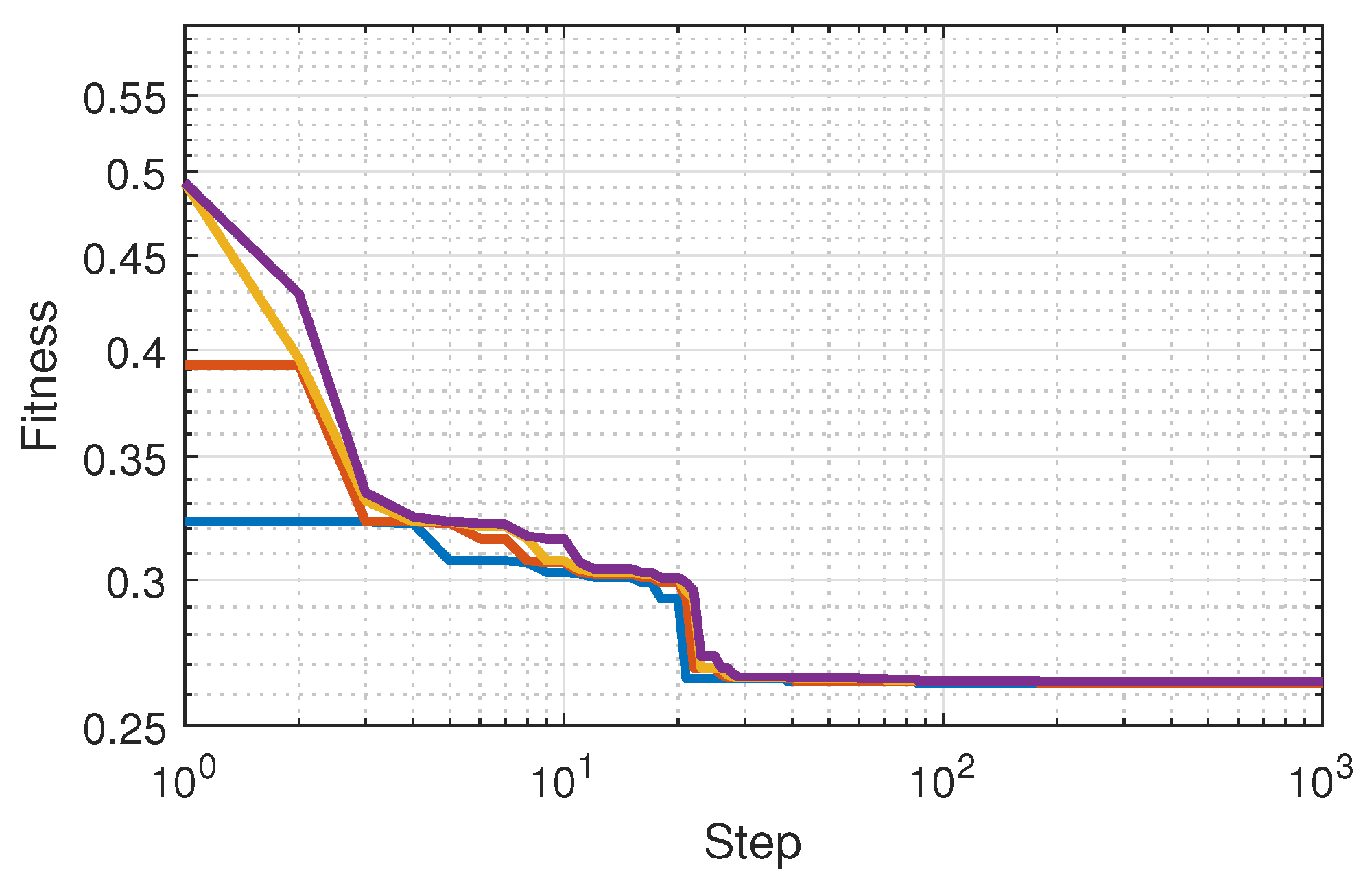
Fitness $j:1\to m$

For each individual $j:1\to m$, the corresponding set of genes, indicated in the rows of (11), are used as coefficients of the covariance matrices of the EKF presented in Section 3.2. For each set of genes, during the evolution of the corresponding EKF algorithm, the fitness function (12) for $j=0$ is continuously updated. This function is the root mean square error between the actual voltage and the estimated output voltage of the EKF at each computation step k.

$$\begin{array}{c}\hfill fitness\left({\mathbf{X}}_{j,i}\right)=\sqrt[2]{\frac{1}{n}\sum {(v_{B_{real}}-{\widehat{v}}_{B_{EKF}})}^2}\end{array}$$

(12)

This choice of the fitness function (12) is crucial for obtaining the correct results of the optimization process. After applying the EKF to the available measured data, by using the m sets of genes as covariance coefficients, an initial vector containing the results of the fitness function is obtained.

$$\begin{array}{c}\hfill \left[\begin{array}{c}fitness\left({\mathbf{X}}_{1,0}\right)\\ ⋮\\ fitness\left({\mathbf{X}}_{m,0}\right)\end{array}\right]\end{array}$$

(13)

(3)

Selection

With the selection function, the process enters in an iterative cycle, where each i cycle represents a new generation of individuals. In this function, the two individuals having the lowest fitness value are selected from the current population ${\mathbf{X}}_{j,i}$ and defined as “parents”. To avoid the premature problem, two parents with the same genes cannot be chosen. In this case, the following individual is taken.

$$\begin{array}{c}\hfill \left[{\mathbf{X}}_{1,i}\right]\left[{\mathbf{X}}_{2,i}\right]\end{array}$$

(14)

(4)

Crossover

The crossover function generates l “children” individuals ${\mathbf{S}}_{j,i}$ using a linear combination of the two previously selected parents. The Crossover Function matrix ${\mathbf{Q}}_C$ and the generated l children are defined as:

$$\begin{array}{c}\hfill \left[\begin{array}{c}{\mathbf{S}}_{1,i}\\ ⋮\\ {\mathbf{S}}_{l,i}\end{array}\right]=\left[{\mathbf{Q}}_C\right]=\left[\begin{array}{c}{\mathbf{X}}_{1,i}\\ {\mathbf{X}}_{2,i}\end{array}\right]\end{array}$$

(15)

Among the several known crossover functions [39], two have been chosen: the one-point crossover and the standard crossover. Therefore, by applying these two crossover functions to the two selected parents, four children are generated $l=4$.

(5)

Mutation

In the evolutionary process, some random mutations appear between two generations. Gene mutation of the children occurs with a predefined probability p, and in case of mutation, the new value is randomly chosen inside a predefined domain. The domain is in discrete form and is represented by ${10}^s$, where the s ranges from $-15$ to 4 and the step $=1$, so the whole domain is ${10}^{-15}\to {10}^4$. The domain is defined so that all “’reasonable” points are inside. In this way, there are no points fixed by the choice of the domain itself. This function is called: Mutation Function ${\mathbf{Q}}_m$.

$$\begin{array}{c}\hfill \left[\begin{array}{c}{\mathbf{S}}_{1,i}\\ ⋮\\ {\mathbf{S}}_{l,i}\end{array}\right]=\left[{\mathbf{Q}}_m\right]=\left[\begin{array}{c}{\mathbf{S}}_{1,i}\\ ⋮\\ {\mathbf{S}}_{l,i}\end{array}\right]\end{array}$$

(16)

Once the new vector of children individuals ${\mathbf{S}}_{j,i}$ (with $j:1\to l$) is obtained, a sequence of l EKF elaborations is performed. Each EKF elaboration uses the new covariance coefficients given by the children’s genes and by using the same reference measured cell quantities. During the evolution of each EKF, the new fitness values for the children are calculated by using the same fitness function introduced in (12).

$$\begin{array}{c}\hfill \left[\begin{array}{c}fitness\left({\mathbf{S}}_{1,i}\right)\\ ⋮\\ fitness\left({\mathbf{S}}_{l,i}\right)\end{array}\right]\end{array}$$

(17)

(6)

Population

Update The next generation of the population $i+1$ is composed by a combination of parents and children, where the l worse parents are substituted by the children. In this way, the maximum amount of elements is always m. In this case, the number of parents m are 20, as the number of children l are 4 and the retained parents are 16.

$$\begin{array}{c}\hfill \left[\begin{array}{c}\left({\mathbf{X}}_{1,i+1}\right)\\ ⋮\\ \left({\mathbf{X}}_{m-l,i+1}\right)\\ \left({\mathbf{X}}_{m-l+1,i+1}\right)\\ ⋮\\ \left({\mathbf{X}}_{m,i+1}\right)\end{array}\right]=\left[\begin{array}{c}\left({\mathbf{X}}_{1,i}\right)\\ ⋮\\ \left({\mathbf{X}}_{m-l,i}\right)\\ \left({\mathbf{S}}_{1,i}\right)\\ ⋮\\ \left({\mathbf{S}}_{l,i}\right)\end{array}\right]\end{array}$$

(18)

The resulting fitness functions of the new population are simply obtained by merging the corresponding fitness functions of selected parents and children.

The fitness vector is used at the next iteration $i+1$ for the selection step, which selects the two parents of the new generation. It is worth noting that, with this genetic algorithm, at each new generation, the EKF elaboration is limited to the new l individuals (children only) of the population. The genetic algorithm continues to evolve, generation after generation, until a satisfactory result is achieved. This is represented by a target for the fitness value.

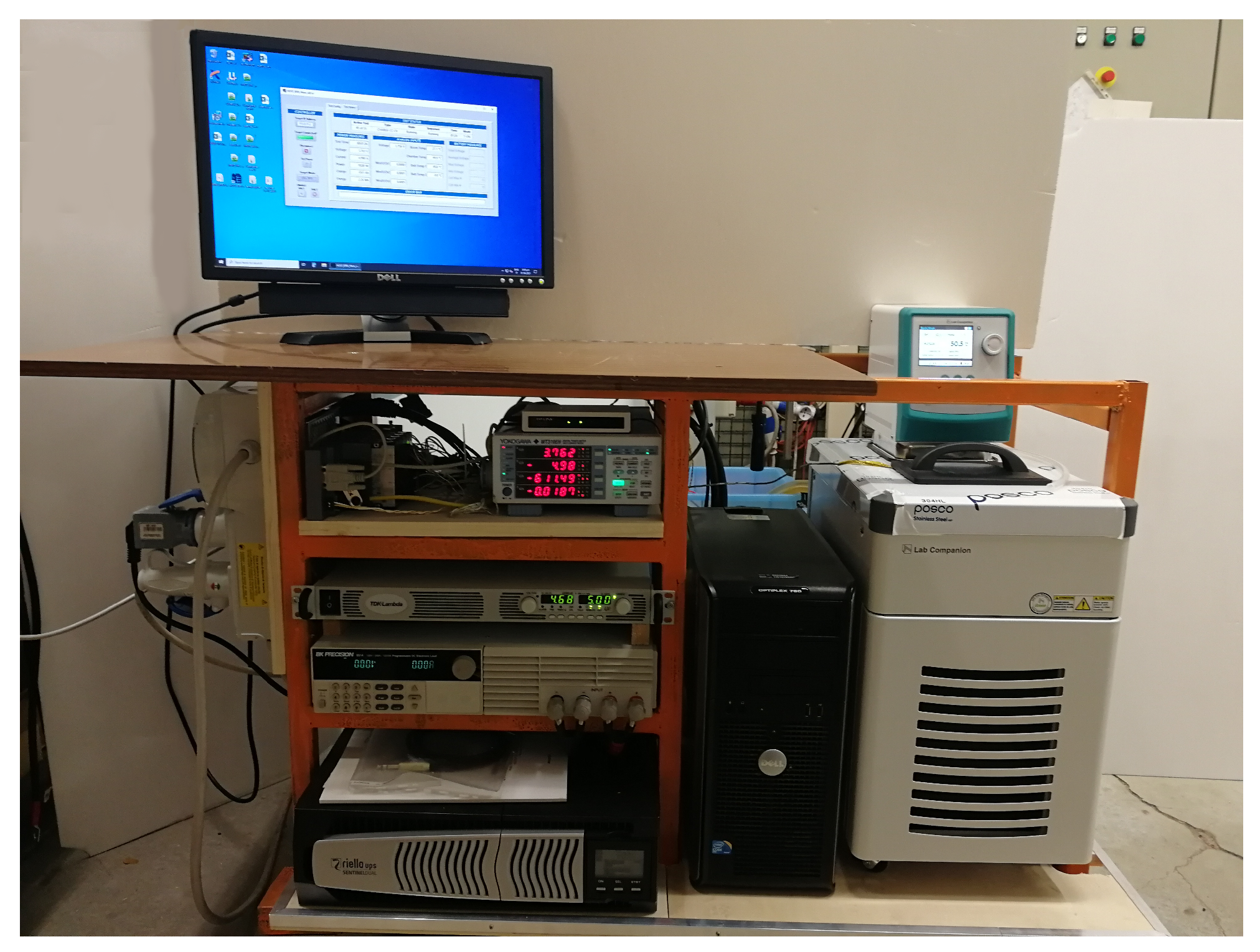
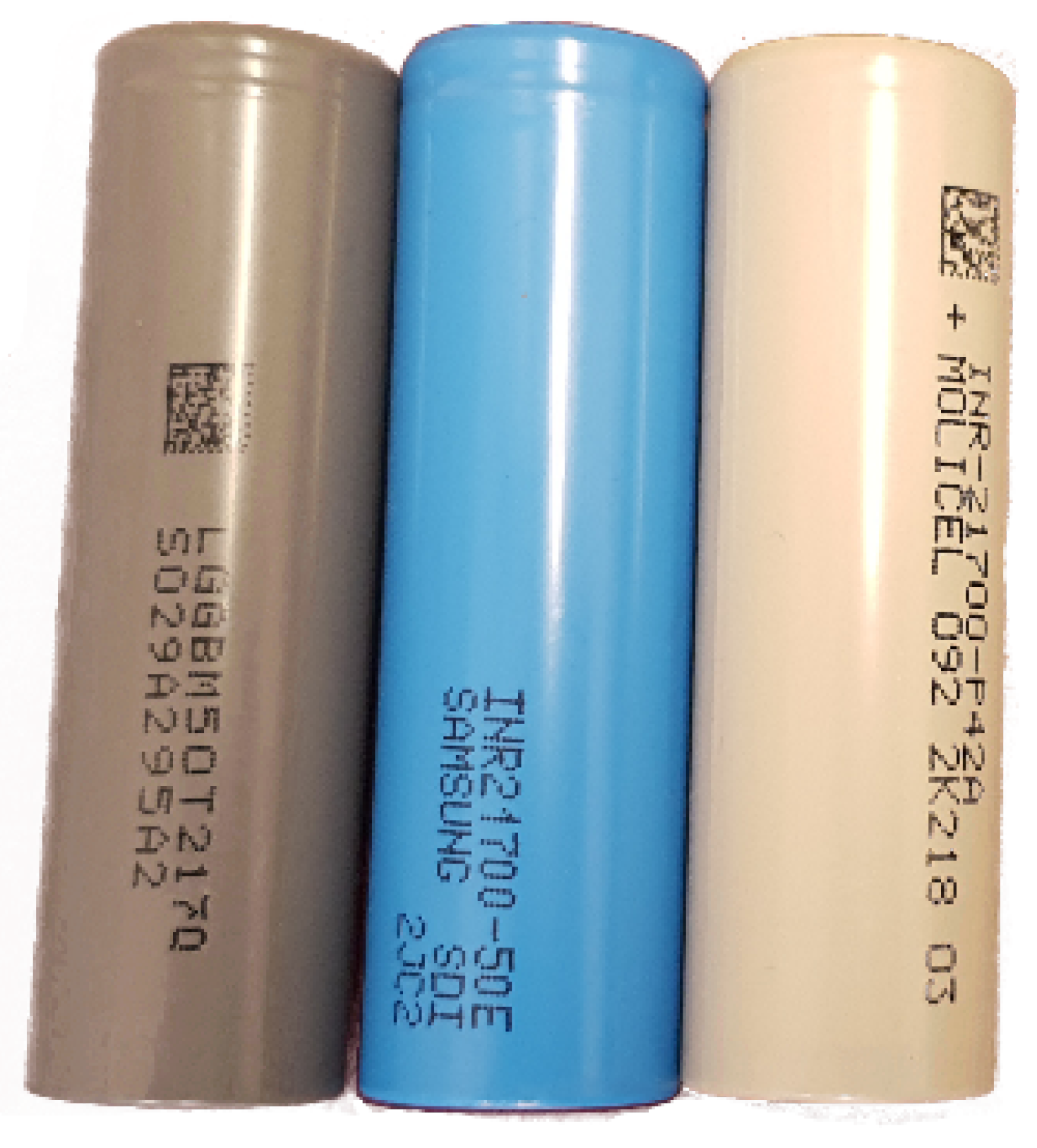
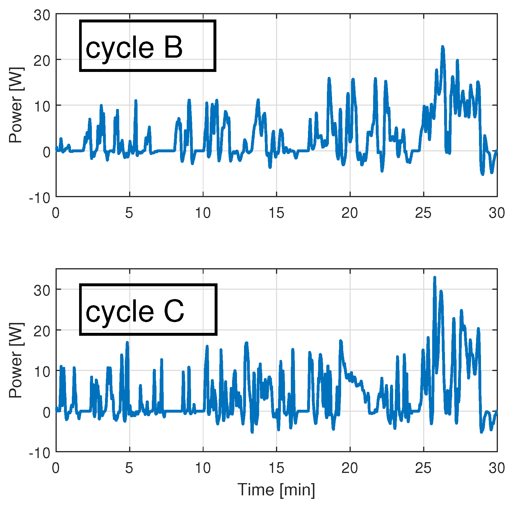
4. Experimental Tests

In this section, numerical details and results of the genetic algorithm optimization procedure are given. The performance of the resulting genetically optimized extended Kalman filter for the estimation of the cell parameters is also reported. In the result analysis, particular attention is paid to the accuracy of $R_0$, because of its relevance in the SOH estimation processes.

4.1. Execution of the Optimization Procedure

The optimization procedure described in Section 3.3 is implemented by using the testing cycle “A” shown in Figure 1, which discharges the cell from from $100\%$ to $0\%$ SOC. This testing cycle is applied to seven combinations of cell models and aging given in Table 2. The genes selected by the genetic optimization, representing the coefficients of the EKF covariance matrix, are given in

Table 5. Coefficients of the covariance matrices found by the genetic algorithm.

Cell	Cycles	${\mathit{Q}}_{1,1}$	${\mathit{Q}}_{2,2}$	${\mathit{Q}}_{3,3}$	${\mathit{Q}}_{4,4}$	${\mathit{R}}_{1,1}$
LG	1-A	${10}^{-2}$	${10}^{-6}$	${10}^{-3}$	${10}^4$	${10}^{-2}$
SAMSUNG	1-A	${10}^{-9}$	${10}^{-12}$	${10}^{-9}$	${10}^{-2}$	${10}^{-9}$
MOLICEL	1-A	${10}^{-5}$	${10}^{-8}$	${10}^{-6}$	${10}^1$	${10}^{-5}$

.

Figure 5 shows the score of the four best elements in the population at each iteration of the optimization procedure. After about 100 generations, the fitness tends to an asymptote, therefore, there is no reason to extend the number of iterations far beyond this value, and so the maximum number of iteration is fixed at 1000.

For demonstrating the algorithm power, all the possible combinations are considered. There are 5 genes, and each of them can assume 20 different values from ${10}^{-15}$ to ${10}^4$, so all the possible combinations are: ${20}^5=3,200,000$. With the proposed algorithm, only four children of each generation are selected and, after 1000 iterations, the score no longer decreases. With this approach, the tested solutions are only: $4\times 1000=4000$; that is 800 times less than the total number of combinations. The accuracy reached is independent on the selection of the starting point, so it can be arbitrarily chosen. The accuracy is not related to the starting point because of the genetic algorithm itself, as in, if the number of iterations and individuals is high, the founded minimum is not a function of the particular starting point.

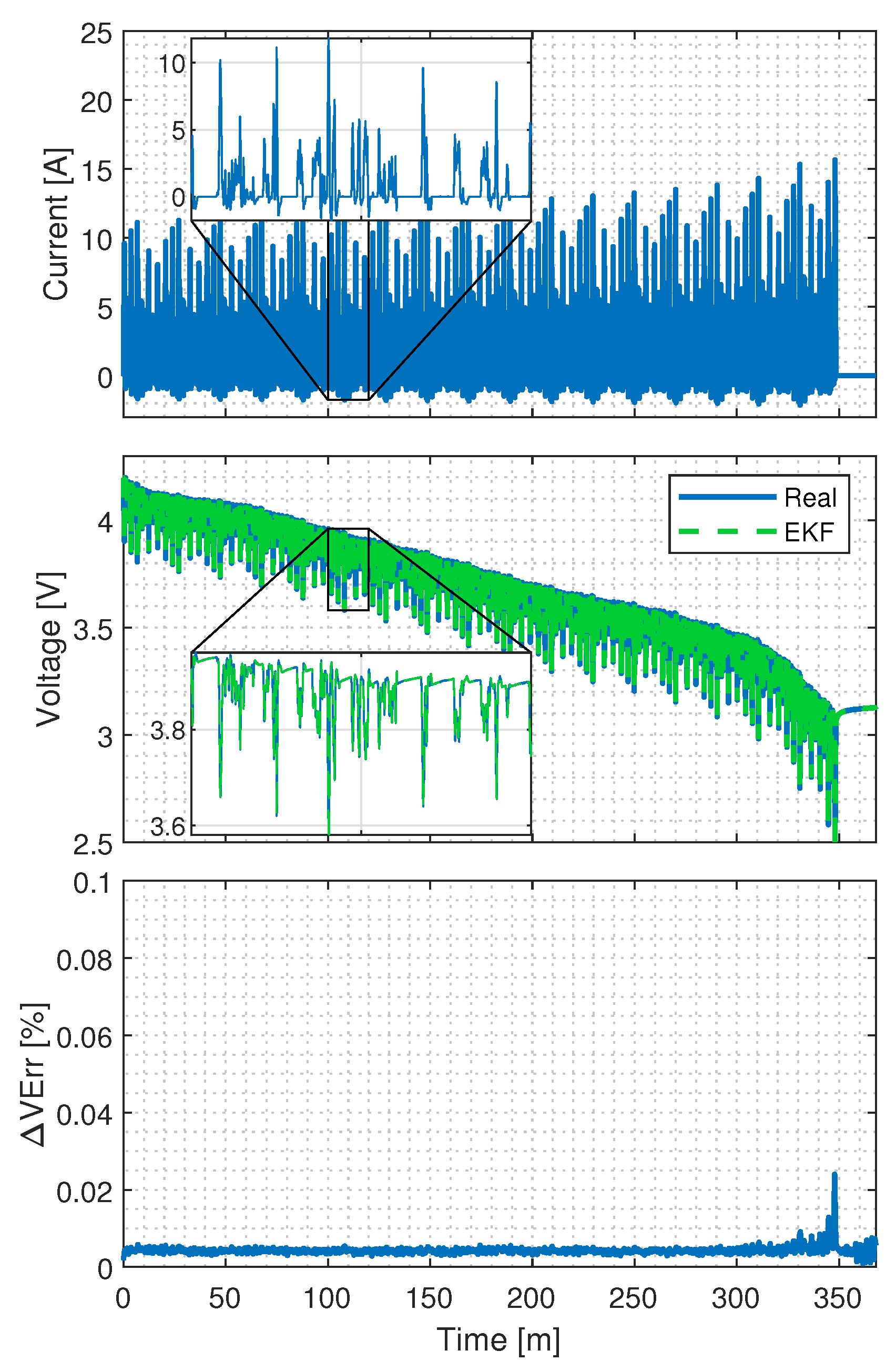
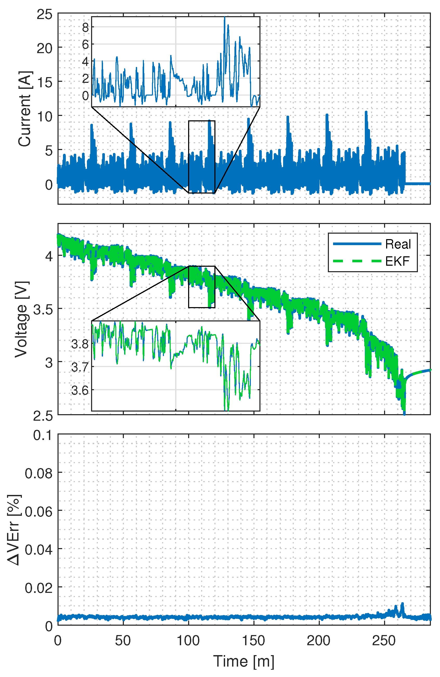
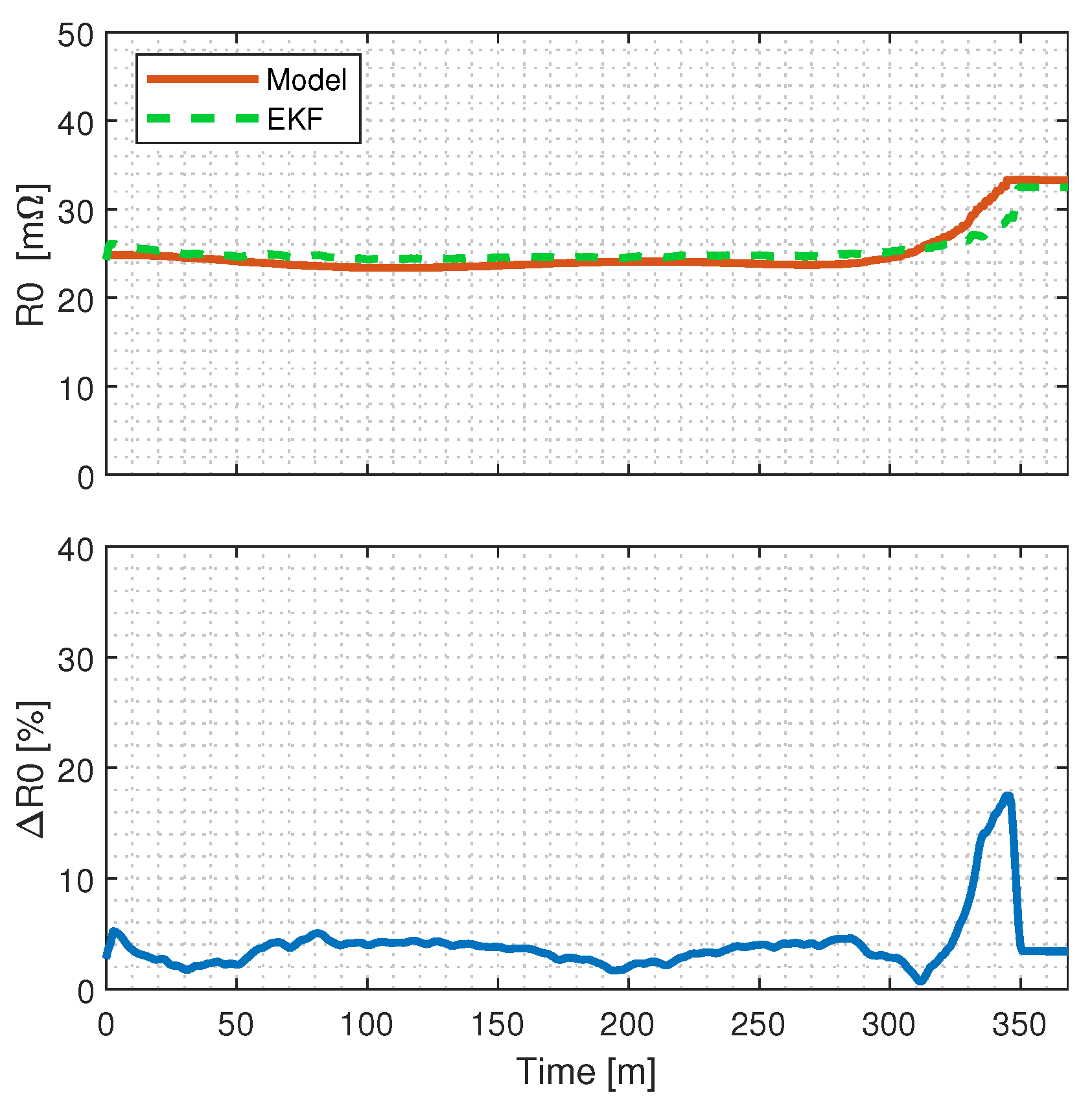
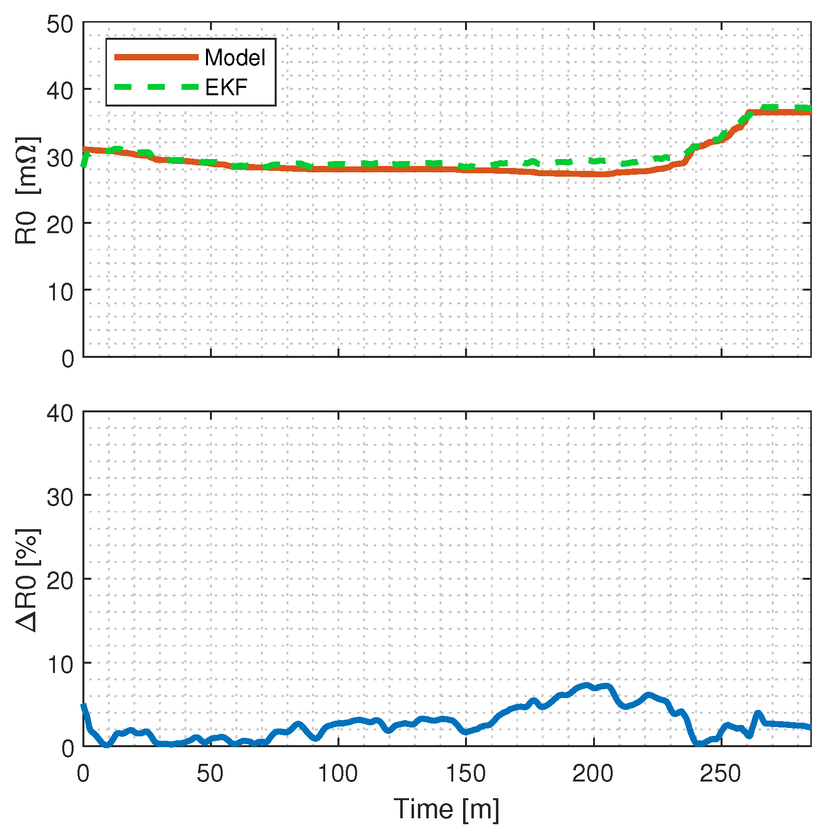
4.2. EKF Testing

The resulting EKF with genetic optimized covariance matrices are tested using the reference scheme of Figure 6. According to this scheme, the same current profile is applied to the actual cell, to the reference model and to the proposed genetically optimized extended Kalman filter. With this approach, the output of the EKF can be compared with the real voltage obtained from the experimental data and with the $R_0$ value given by the reference model considered as the true value of the resistance. For analyzing the results obtained by the proposed EKF in the various tests, both instantaneous and average errors on the output voltage and on the DC resistance $R_0$ were calculated.

The voltage error is calculated between the real voltage and the filter estimated one. The value is normalized by the nominal voltage of each cell, as in (19), (21) and (23), due to the small error value on RMSE and ME, the value are expressed in parts per million(ppm). The error is calculated as a comparison between the value estimated by the EKF and the true value of the model presented in Section 2. This value is normalized by the resistance value at $SOC=50\%$, as in (20), (22) and (24), where there is a plateau of the resistance value. This choice allows us to compare the accuracy of the method with different cells.

$$\begin{array}{c}\hfill \begin{array}{c}\hfill V_{RMS}=\frac{\sqrt[2]{\frac{1}{n}\sum {(v_{B_{real}}-{\widehat{v}}_{B_{EKF}})}^2}}{v_{nom}}\end{array}\end{array}$$

(19)

$$\begin{array}{c}\hfill \begin{array}{c}\hfill R_{RMS}=\frac{\sqrt[2]{\frac{1}{n}\sum {(R_{0_{model}}-{\widehat{R}}_{0_{EKF}})}^2}}{R_{0_{model}}{|}_{SOC=50\%}}\end{array}\end{array}$$

(20)

$$\begin{array}{c}\hfill \begin{array}{c}\hfill V_{Mean}=\frac{\frac{1}{n}\sum (v_{B_{real}}-{\widehat{v}}_{B_{EKF}})}{v_{nom}}\end{array}\end{array}$$

(21)

$$\begin{array}{c}\hfill \begin{array}{c}\hfill R_{Mean}=\frac{\frac{1}{n}\sum (R_{0_{model}}-{\widehat{R}}_{0_{EKF}})}{R_{0_{model}}{|}_{SOC=50\%}}\end{array}\end{array}$$

(22)

$$\begin{array}{c}\hfill \begin{array}{c}\hfill V_{Max}=\frac{MAX|v_{B_{real}}-{\widehat{v}}_{B_{EKF}}|}{v_{nom}}\end{array}\end{array}$$

(23)

$$\begin{array}{c}\hfill \begin{array}{c}\hfill R_{Max}=\frac{MAX|R_{0_{model}}-{\widehat{R}}_{0_{EKF}}|}{R_{0_{model}}{|}_{SOC=50\%}}\end{array}\end{array}$$

(24)

The performance of the EKF with the covariance coefficients, obtained from the optimization process and listed in Table 5, are verified on cycle “A”, the same used in the optimization process, and on two different current profiles called cycle “B” (Figure 7 top) and cycle “C” (Figure 7 bottom). For the LG and Samsung cells, the EKF with the optimized coefficients was also tested on aged samples with cycle “A”.

Figure 8 shows the performance of the EKF, with the proposed genetically optimized covariance matrix, in estimating the cell voltage, performed on a new LG cell using cycle “A”. Figure 9 shows the result obtained on a different cell at the end of its life, performed on cycle “C”.

Figure 10 shows the performance of the EKF, with the proposed genetically optimized covariance matrix, in the estimation of the internal resistance, carried out on a new LG cell, using cycle “A”. These tests prove that the estimation error is far below $5\%$ for most of the $SOC$ values. It is also possible to appreciate the response time of the filter, which takes a few seconds from the start up to converge to the correct value.

Table 6. Error comparison obtained with the new cell. Voltage $V_B$ error estimation.

Manufacturer	Cycles Number	RMSE (19) (ppm)	ME (21) (ppm)	MAE (23) (%)
LG	1-A	80.41	3.52	0.19
LG	1-B	65.17	1.94	0.07
LG	1-C	78.53	0.77	0.09
Molicell	1-A	58.18	−1.73	0.29
Molicell	1-B	61.12	−2.39	0.06
Molicell	1-C	54.69	−0.25	0.05
Samsung	1-A	57.72	−3.30	0.17

,

Table 7. Error comparison obtained with the new cell. Resistance $R_0$ error estimation.

Manufacturer	Cycles Number	RMSE (19) (ppm)	ME (21) (ppm)	MAE (23) (%)
LG	1-A	4.80	1.80	41.11
LG	1-B	5.61	1.84	41.70
LG	1-C	21.28	−3.17	82.50
Molicell	1-A	12.80	−1.17	58.38
Molicell	1-B	8.02	−1.34	89.50
Molicell	1-C	19.13	−10.55	61.74
Samsung	1-A	4.14	2.18	51.35

,

Table 8. Error comparison obtained with the aged cell. Voltage $V_B$ error estimation.

Manufacturer	Cycles Number	RMSE (19) (ppm)	ME (21) (ppm)	MAE (23) (%)
LG	100-B	65.15	−3.86	0.23
LG	200-B	61.49	−4.33	0.09
Samsung	100-A	66.69	−4.86	0.21
Samsung	300-A	69.68	−5.43	0.24
Samsung	500-A	60.29	−2.61	0.16
Samsung	500-B	58.83	−1.79	0.10
Samsung	500-C	56.94	−2.84	0.09

and

Table 9. Error comparison obtained with the aged cell. Resistance $R_0$ error estimation.

Manufacturer	Cycles Number	RMSE (19) (ppm)	ME (21) (ppm)	MAE (23) (%)
LG	100-B	2.83	−1.62	56.51
LG	200-B	3.60	−0.91	60.78
Samsung	100-A	3.00	0.53	46.85
Samsung	300-A	3.19	1.68	53.27
Samsung	500-A	5.40	1.95	57.08
Samsung	500-B	5.32	4.20	57.08
Samsung	500-C	3.50	2.63	57.08

give an overview of the estimation accuracy of the output voltage and internal resistance of the proposed method for the considered cell models and aging conditions. For both output voltage and internal resistance, the results are given in terms of root mean square error (RMSE), mean error (ME) and maximum absolute error (MAE) and are used for evaluating the proposed models.

The result obtained for voltage estimation, with optimized covariance matrix coefficients, can be compared with the value in Table 3 where the literature results are given. This method can achieve good accuracy on the internal resistance $R_0$ estimation.

The maximum error is high due to the initial value of $R_0$, but the filter quickly converges to the true value as shown in Figure 10 and Figure 11. This error can be reduced by initializing if the initial conditions are known, or if the measurement in the previous cycle is available. With such a low error value, it is interesting to estimate the internal resistance in order to evaluate the SOH of the cell, which would not be possible with higher errors. Therefore, the proposed genetically optimized selection of the covariance matrix coefficients, implemented only once per cell model, guarantees a correct estimation even when the cell parameters are different from the initial ones, and it is possible to determine the coefficients of the matrices by carrying out tests with a new cell and then using these values throughout its life. Based on the definition of the SOH Equation (25) proposed by many authors [9,41], it is possible to obtain the SOH where the $R_{act}$ and $R_{new}$ are the actual and the new value of the resistance, respectively.

$$SOH\left(t\right)=\frac{R_{act}-R_{new}}{R_{new}}\times 100$$

(25)

The value of the internal resistance $R_0$ increases by $20\%$ after 200 cycles for the LG sample and $40\%$ after 500 cycles for the Samsung sample. The average error on the estimate of $R_0$ is less than $4\%$, therefore it is possible to achieve a high level of accuracy on the SOH estimation.

5. Conclusions

This paper introduces a new procedure to determine the covariance matrix coefficients used in the extended Kalman filter by means of an optimization procedure based on a genetic algorithm. A form of the EKF, with carefully chosen state variables, the genetic algorithm and the implementation of the optimization procedure are described in detail in the paper. The performance of the proposed approach has been validated against new and aged Li-Ion cells of different models. For measuring the accuracy of the proposed GO-EKF, a reference model, derived from a cell testing procedure, is required. It is demonstrated that both cell output voltage and cell internal resistance can be estimated with significantly high accuracy, at any aging condition of the cell. These results are obtained by means of an optimization procedure, which is carried out only once per cell. In this way, it is possible to demonstrate that only one optimization is needed to estimate the SOH during the whole cell life. The optimization procedure can be performed at any aging condition and does not require any specific current profile and, therefore, it can be implemented during the normal operation of the cells. Additional optimizations were carried out with different initial values in order to verify whether the found value is a local or a global minimum. Since each found value is near to the others, this point can be considered as a global minimum. This feature is considered of particular interest for the correct modeling of an aged cell, with unknown history. The proposed methodology allows us to obtain a very accurate estimation of the internal series resistance, representing a remarkable starting point for the development of algorithms for the cell’s SOH estimation. The procedure has been developed to be suitable for embedding within a BMS, allowing for the real-time estimation of the parameters during normal operation of the battery, without specific tests. The method requires a small amount of memory because it stores a fixed number of elements in each iteration. The accuracy obtained and the portability of the optimization method to unknown and aged cells, allow us to avoid the empirical tuning of the covariance matrix coefficients, placing the proposed GO-EKF far beyond the other estimation methods currently available in the literature. Future work on this subject will require verification of the method performance if the optimization is performed at any cell age, and will assess the method performance at different cells temperatures.

References

- Plett, G.L. Battery Management Systems, Volume II: Equivalent-Circuit Methods; Artech House: Norwood, MA, USA, 2016. [Google Scholar]
- Smith, K.; Shi, Y.; Santhanagopalan, S. Degradation mechanisms and lifetime prediction for lithium-ion batteries—A control perspective. In Proceedings of the 2015 American Control Conference (ACC), Chicago, IL, USA, 1–3 July 2005; pp. 728–730. [Google Scholar] [CrossRef]
- Plett, G.L. Battery Management Systems, Volume I: Battery Modeling; Artech House: Norwood, MA, USA, 2015. [Google Scholar]
- Campestrini, C.; Heil, T.; Kosch, S.; Jossen, A. A comparative study and review of different Kalman filters by applying an enhanced validation method. J. Energy Storage 2016, 8, 142–159. [Google Scholar] [CrossRef]
- Dong, H.; Jin, X.; Lou, Y.; Wang, C. Lithium-ion battery state of health monitoring and remaining useful life prediction based on support vector regression-particle filter. J. Power Sources 2014, 271, 114–123. [Google Scholar] [CrossRef]
- Li, W.; Liang, L.; Liu, W.; Wu, X. State of Charge Estimation of Lithium-Ion Batteries Using a Discrete-Time Nonlinear Observer. IEEE Trans. Ind. Electron. 2017, 64, 8557–8565. [Google Scholar] [CrossRef]
- Jokić, I.; Zečević, Z.; Krstajić, B. State-of-charge estimation of lithium-ion batteries using extended Kalman filter and unscented Kalman filter. In Proceedings of the 2018 23rd International Scientific-Professional Conference on Information Technology (IT), Zabljak, Montenegro, 19–24 February 2018; pp. 1–4. [Google Scholar] [CrossRef]
- Cong, J.; Wang, S.; Wu, B.; Fernandez, C.; Xiong, X.; Coffie-Ken, J. A state-of-charge estimation method of the power lithium-ion battery in complex conditions based on adaptive square root extended Kalman filter. Energy 2021, 219, 119603. [Google Scholar] [CrossRef]
- Andrea, D. Battery Management Systems for Large Lithium-Ion Battery Packs; Artech House: Boston, MA, USA, 2010. [Google Scholar]
- Yu, Q.; Xiong, R.; Lin, C.; Shen, W.; Deng, J. Lithium-Ion Battery Parameters and State-of-Charge Joint Estimation Based on H-Infinity and Unscented Kalman Filters. IEEE Trans. Veh. Technol. 2017, 66, 8693–8701. [Google Scholar] [CrossRef]
- Guha, A.; Patra, A. State of Health Estimation of Lithium-Ion Batteries Using Capacity Fade and Internal Resistance Growth Models. IEEE Trans. Transp. Electrif. 2018, 4, 135–146. [Google Scholar] [CrossRef]
- Ramachandran, R.; Ganeshaperumal, D.; Subathra, B. Parameter Estimation of Battery Pack in EV using Extended Kalman Filters. In Proceedings of the 2019 IEEE International Conference on Clean Energy and Energy Efficient Electronics Circuit for Sustainable Development (INCCES), Krishnankoil, India, 18–20 December 2019; pp. 1–5. [Google Scholar] [CrossRef]
- Liuyi, L.; Wei, Y. State-of-Charge and State-of-Health Estimation for Lithium-Ion Batteries Based on Dual Fractional-Order Extended Kalman Filter and Online Parameter Identification. IEEE Access 2021, 9, 47588–47602. [Google Scholar] [CrossRef]
- Gholizadeh, M.; Salmasi, F.R. Estimation of State of Charge, Unknown Nonlinearities, and State of Health of a Lithium-Ion Battery Based on a Comprehensive Unobservable Model. IEEE Trans. Ind. Electron. 2014, 61, 1335–1344. [Google Scholar] [CrossRef]
- Remmlinger, J.; Buchholz, M.; Meiler, M.; Bernreuter, P.; Dietmayer, K. State-of-health monitoring of lithium-ion batteries in electric vehicles by on-board internal resistance estimation. J. Power Sources 2011, 196, 5357–5363. [Google Scholar] [CrossRef]
- Rossi, C.; Pontara, D.; Falcomer, C.; Bertoldi, M. Simplified Parameters Estimation forthe Dual Polarization Model of Lithium-Ion Cell. In Proceedings of the ELECTRIMACS 2019, Salerno, Italy, 21–23 May 2019; Zamboni, W., Petrone, G., Eds.; Lecture Notes in Electrical Engineering. Springer: Cham, Switzerland, 2020; Volume 697, pp. 129–144. [Google Scholar] [CrossRef]
- Gao, L.; Liu, S.; Dougal, R.A. Dynamic lithium-ion battery model for system simulation. IEEE Trans. Components Packag. Technol. 2002, 25, 495–505. [Google Scholar] [CrossRef] [Green Version]
- Gao, Z.; Chin, C.S.; Woo, W.L.; Jia, J.; Toh, W.D. Lithium-ion battery modeling and validation for smart power system. In Proceedings of the 2015 International Conference on Computer, Communications, and Control Technology (I4CT), Kuching, Malaysia, 21–23 April 2015; pp. 269–274. [Google Scholar] [CrossRef]
- Ahmed, R.; Gazzarri, J.; Onori, S.; Habibi, S.; Jackey, R.; Rzemien, K.; Tjong, J.; LeSage, J. Model-Based Parameter Identification of Healthy and Aged Li-ion Batteries for Electric Vehicle Applications. SAE Int. J. Altern. Powertrains 2015, 4, 233–247. [Google Scholar] [CrossRef] [Green Version]
- Damiano, A.; Musio, C.; Marongiu, I. Experimental validation of a dynamic energy model of a battery electric vehicle. In Proceedings of the 2015 International Conference on Renewable Energy Research and Applications (ICRERA), Palermo, Italy, 22–25 November 2015; pp. 803–808. [Google Scholar] [CrossRef]
- Haykin, S. Kalman Filtering and Neural Networks; John Wiley & Sons: New York, NY, USA, 2001. [Google Scholar]
- Plett, G.L. Extended Kalman filtering for battery management systems of LiPB-based HEV battery packs Part 1. Background. J. Power Sources 2004, 134, 252–261. [Google Scholar] [CrossRef]
- Plett, G.L. Extended Kalman filtering for battery management systems of LiPB-based HEV battery packs: Part 2. Modeling and identification. J. Power Sources 2004, 134, 262–276. [Google Scholar] [CrossRef]
- Han, J.; Kim, D.; Sunwoo, M. State-of-charge estimation of lead-acid batteries using an adaptive extended Kalman filter. J. Power Sources 2009, 188, 606–612. [Google Scholar] [CrossRef]
- Vasebi, A.; Partovibakhsh, M.; Bathaee, S.M.T. A novel combined battery model for state-of-charge estimation in lead-acid batteries based on extended Kalman filter for hybrid electric vehicle applications. J. Power Sources 2007, 174, 30–40. [Google Scholar] [CrossRef]
- Vasebi, A.; Bathaee, S.; Partovibakhsh, M. Predicting state of charge of lead-acid batteries for hybrid electric vehicles by extended Kalman filter. Energy Convers. Manag. 2008, 49, 75–82. [Google Scholar] [CrossRef]
- Liu, Z.; Li, Z.; Zhang, J.; Su, L.; Ge, H. Accurate and Efficient Estimation of Lithium-Ion Battery State of Charge with Alternate Adaptive Extended Kalman Filter and Ampere-Hour Counting Methods. Energies 2019, 12, 757. [Google Scholar] [CrossRef] [Green Version]
- Bhangu, B.S.; Bentley, P.; Stone, D.A.; Bingham, C.M. Observer techniques for estimating the state-of-charge and state-of-health of VRLABs for hybrid electric vehicles. In Proceedings of the 2005 IEEE Vehicle Power and Propulsion Conference, Chicago, IL, USA, 7–9 September 2005; 10p. [Google Scholar] [CrossRef] [Green Version]
- Zhang, F.; Liu, G.; Fang, L. A battery State of Charge estimation method with extended Kalman filter. In Proceedings of the 2008 IEEE/ASME International Conference on Advanced Intelligent Mechatronics, Xi’an, China, 2–5 July 2008; pp. 1008–1013. [Google Scholar] [CrossRef]
- He, H.; Qin, H.; Sun, X.; Shui, Y. Comparison Study on the Battery SoC Estimation with EKF and UKF Algorithms. Energies 2013, 6, 5088–5100. [Google Scholar] [CrossRef]
- Zarchan, P.; Musoff, H. Fundamentals of Kalman Filtering: A Practical Approach, 3rd ed.; American Institute of Aeronautics and Astronautics: Reston, VA, USA, 2009. [Google Scholar]
- Biswas, A.; Gu, R.; Kollmeyer, P.; Ahmed, R.; Emadi, A. Simultaneous State and Parameter Estimation of Li-Ion Battery with One State Hysteresis Model Using Augmented Unscented Kalman Filter. In Proceedings of the 2018 IEEE Transportation Electrification Conference and Expo (ITEC), Long Beach, CA, USA, 13–15 June 2018; pp. 1065–1070. [Google Scholar] [CrossRef]
- Yang, S.; Zhou, S.; Hua, Y.; Zhou, X.; Liu, X.; Pan, Y.; Ling, H.; Wu, B. A parameter adaptive method for state of charge estimation of lithium-ion batteries with an improved extended Kalman filter. Sci. Rep. 2021, 11, 2045–2322. [Google Scholar] [CrossRef]
- He, H.; Xiong, R.; Zhang, X.; Sun, F.; Fan, J. State-of-Charge Estimation of the Lithium-Ion Battery Using an Adaptive Extended Kalman Filter Based on an Improved Thevenin Model. IEEE Trans. Veh. Technol. 2011, 60, 1461–1469. [Google Scholar] [CrossRef]
- Xia, B.; Wang, H.; Tian, Y.; Wang, M.; Sun, W.; Xu, Z. State of Charge Estimation of Lithium-Ion Batteries Using an Adaptive Cubature Kalman Filter. Energies 2015, 8, 5916–5936. [Google Scholar] [CrossRef] [Green Version]
- Ayzah, A.N.; Joelianto, E.; Widyotriatmo, A. State of Charge (SoC) and State of Health (SoH) Estimation of Lithium-Ion Battery Using Dual Extended Kalman Filter Based on Polynomial Battery Model. In Proceedings of the 2019 6th International Conference on Instrumentation, Control, and Automation (ICA), Bandung, Indonesia, 31 July–2 August 2019; pp. 88–93. [Google Scholar] [CrossRef]
- Nikolaos, W.; Adermann, J.; Frericks, A.; Pak, M.; Reiter, C.; Lohmann, B.; Lienkamp, M. Revisiting the dual extended Kalman filter for battery state-of-charge and state-of-health estimation: A use-case life cycle analysis. J. Energy Storage 2018, 19, 73–87. [Google Scholar] [CrossRef]
- Goldberg, D.E. Genetic Algorithms in Search, Optimization and Machine Learning; Addison-Wesley: Boston, MA, USA, 1989. [Google Scholar]
- Sivanandam, S.N.; Deepa, S.N. Introduction to Genetic Algorithms; Springer: Berlin/Heidelberg, Germany; New York, NY, USA, 2007. [Google Scholar]
- Ahmad, F.; Isa, N.A.M.; Osman, M.K.; Hussain, Z. Performance comparison of gradient descent and Genetic Algorithm based Artificial Neural Networks training. In Proceedings of the 2010 10th International Conference on Intelligent Systems Design and Applications, Cairo, Egypt, 29 November–1 December 2010; pp. 604–609. [Google Scholar] [CrossRef]
- Hu, X.; Feng, F.; Liu, K.; Zhang, L.; Xie, J.; Liu, B. State estimation for advanced battery management: Key challenges and future trends. Renew. Sustain. Energy Rev. 2019, 114, 109334. [Google Scholar] [CrossRef]