Ultra-Short-Term Wind Power Combined Prediction Based on Complementary Ensemble Empirical Mode Decomposition, Whale Optimisation Algorithm, and Elman Network

Abstract

Accurate wind power forecasting helps relieve the regulation pressure of a power system, which is of great significance to the power system’s operation. However, achieving satisfactory results in wind power forecasting is highly challenging due to the random volatility characteristics of wind power sequences. This study proposes a novel ultra-short-term wind power combined prediction method based on complementary ensemble empirical mode decomposition, the whale optimization algorithm (WOA), and the Elman neural network model. The model can not only solve the phenomenon of easy modal mixing in decomposition but also avoid the problems of reconstruction error and low efficiency in the decomposition process. Furthermore, a new metaheuristic algorithm, WOA, was introduced to optimize the model and improve the accuracy of wind power prediction. Considering a wind farm as an example, several wind turbines were selected to simulate and analyse wind power by using the established prediction model, and the experimental results suggest that the proposed method has a higher prediction accuracy of ultra-short-term wind power than other prediction models.

1. Introduction

In China, numerous wind turbines have been installed. By the end of August 2021, the wind power generation capacity in China was 14.63 million kW, and the cumulative capacity reached 295.32 million kW, representing a 33.8 increase compared with that in the previous year. Fluctuation, intermittence, and randomness of wind farm output power [1] pose considerable challenges to the stable operation of a power system. Improving the accuracy of wind power prediction is critical for ensuring safe and reliable operation of the power grid and alleviating regulation pressure of the power system [2]. Ultra-short-term wind power prediction refers to the forecast of wind power for the next 15 min to 4 h, with the 15-min prediction interval, and the predicted wind power is rolled the next time [3]. Therefore, developing an ultra-short-term wind power prediction method is critical for improving the accuracy of wind power prediction.

Wind power prediction methods have received considerable research attention. Therefore, numerous methods, including physical [4], time series [5], artificial intelligence [6], and combination methods [7] have been proposed. In [8], a physical method was proposed for wind power prediction based on computational fluid dynamics (CFD) pre calculated flow field. Considering the discrete inflow wind conditions as the boundary conditions, the flow field was obtained, and a database containing critical parameters was established to predict power through the database. To improve the prediction effect of low-resolution NWP and achieve an ideal prediction effect, a method was proposed to deduce the influence of landform and wake effect on the convection field based on NWP and the principle of hydrodynamics. Geographic information (such as terrain and location), meteorological information (such as wind direction, pressure, temperature, and humidity), and organic factors are combined with the physical numerical weather forecast to predict wind power [9]. However, the calculation method is complex and time consuming, and the updating speed of physical numerical weather forecasts is slow. Therefore, obtaining an accurate wind power prediction value is difficult. In [10], a model based on the Markov chain Monte Carlo method was proposed to predict power. In [11], wind power was predicted by establishing a statistical time series model for density prediction. In the time series method, the time series of historical power was used to predict the future wind power output. The modelling is simple and does not depend on the numerical weather forecast data. However, the prediction accuracy is low, and the accuracy decreases rapidly with an increase in the prediction time. In [12], a heterogeneous integrated learning method was proposed in which decision tree and support vector regression analyses were performed to predict wind power. In [13], the least-square support vector machine (LS–SVM) method was used to predict the ultra-short-term wind power load. Algorithms have been modified to improve efficiency and prediction accuracy. Numerous artificial intelligence models have been proposed to establish the nonlinear mapping relationship between input and output variables through numerous historical sample training and predict the future wind power output based on the trained model. With sufficient historical samples, artificial intelligence methods exhibit high prediction accuracy and generalisation. Therefore, these methods are widely used in ultra-short-term, short-term, and medium and long-term wind power prediction. However, because of the limitation of a single prediction model, wind power prediction accuracy is low [14]. To reduce the random fluctuation of wind power, the original wind power sequence is decomposed into several single signals of various frequencies by using signal decomposition technology. Finally, the prediction value of every single signal is reconstructed to realise high-precision wind power prediction. Moreover, the performance of wind power forecasting has been improved with the techniques that combine a single forecasting model with signal decomposition, error correction, and other methods. In [15], wavelet analysis was used to decompose wind power time series, and a power forecasting model based on the wavelet hybrid neural network was established. In [16], an echo state network was used to establish a medium-term wind power prediction model to predict wind power. However, because of the adaptivity of wavelet decomposition and some limitations of ESN in complex dynamic structures, the combined prediction method exhibits certain drawbacks.

Decomposition algorithms are used to capture individual components of the complex data structure and have demonstrated higher accuracy and adaptability in wind power forecasting [17]. In [18], the empirical mode decomposition (EMD) methods were first employed for feature engineering in time series prediction. In [19], an improved hybrid time series decomposition strategy and multi-objective parameter optimization method for wind speed prediction were proposed. In [20], a new system for ensemble probabilistic forecasting of wind speed uncertainty was proposed, a method that accurately quantifies wind speed uncertainty and reduces the operating costs of power systems by improving the efficiency of wind energy utilization. Zhang et al. [21] proposed an ensemble method based on EMD and sample entropy for interval prediction of wind power. In [22], a wind power prediction model based on EMD and Elman was proposed. In the actual data acquisition, the collected wind power signals are usually mixed with white noise, and the modal aliasing phenomenon occurs in the EMD decomposition process; therefore, the ideal wind power subseries cannot be obtained. The improved ensemble empirical modal decomposition (EEMD) can effectively overcome the modal aliasing phenomenon. In [23], a combined prediction method of EEMD and Elman was proposed to effectively eliminate the defects of mode aliasing and reduce the residual noise of the de-composition sequence. Although EEMD can resolve the mode aliasing phenomenon existing in EMD, it can generate residual auxiliary noise, while the white noise added by CEEMD is independent and identically distributed with opposite symbols. The noise added during signal reconstruction will offset each other, which can better reduce the residual auxiliary noise in the original signal and ensure a small reconstruction error after decomposition. In [24], the CEEMD method is adopted to decompose the wind power time series to decrease non-stationarity.

Novel metaheuristic algorithms have been proposed for parameter optimisation of machine learning. In [25], an improved genetic algorithm (GA) was proposed to optimise the Elman neural network model and improve the prediction accuracy of the wind power model. In [26], particle swarm optimisation was used to optimise the parameters of the Elman model. However, this model exhibits low computational efficiency and slow convergence speed in Elman parameter optimisation. A combined prediction model [27] based on the combination of whale optimisation algorithm (WOA) and support vector regression (SVR) was proposed to predict wind speed. The prediction results of the proposed model were compared with the results obtained using the GA and conventional SVR. The analysis showed that WOA outperformed SVR. In [28], a short-term load forecasting method based on WOA and short-term memory (LSTM) neural network was proposed. This method exhibited a faster convergence speed and better forecasting effect than particle swarm optimisation and GA. Therefore, WOA was introduced to perform parameter optimisation in the Elman model.

In the present study, a combined prediction method of ultra-short-term wind power based on complementary ensemble empirical mode decomposition (CEEMD) and WOA-optimised Elman parameters was proposed. CEEMD was used to decompose the historical wind power into sequence components, and the Elman wind power prediction model of each sequence component was established. The weight and threshold of each component Elman model were optimised using WOA, and the predicted value of each component was superimposed to obtain the final predicted value.

2. CEEMD Method

2.1. Empirical Mode Decomposition

Huang et al. proposed the EMD [29] to decompose complex nonlinear and nonstationary signals into finite intrinsic mode functions (IMFs). Each IMF component contains the local characteristics of various time scales of the original signal. In EMD, time series are composed of various oscillation modes at the same time and are accompanied by hidden internal complexity. Therefore, the original sequence is decomposed into the eigenmode function and the residual component, as follows:

$$x(t)={\displaystyle \sum _{i=1}^n{C}_i(t)+r_n(t)}$$

(1)

where n is the number of IMF; $C_i(t)$ represents the i-th IMF; and $r_n(t)$ represents the n-th residual component.

2.2. EEMD

Wu and Huang proposed EEMD to improve modal aliasing [30]. Gaussian white noise was added to the signal to be decomposed. Because white noise exhibits uniform frequency distribution, the signal after adding white noise exhibits continuity on various time scales to effectively avoid the signal aliasing phenomenon caused by the discontinuity of IMF in the process of EMD decomposition. By using the zero-mean characteristic of Gaussian white noise, the average value of the final result was adopted to reduce the change in the amplitude of the decomposition result caused by the added white noise [31]. The specific steps are as follows:

(1)

Determination of the decomposition times and the amplitude standard deviation of Gaussian white noise.

(2)

Gaussian white noise $n_i(t)$ with a mean value of 0 and standard deviation of constant is added to the original sequence $s(t)$ many times as follows:

$$x_i(t)=s(t)+n_i(t)$$

(2)

where $x_i(t)$ is the signal in which Gaussian white noise is added for the i-th time.

(3)

The IMF component $c_{ij}(t)$ and the residual component $r(t)$ are obtained by EEMD decomposition of $x_i(t)$. The result of decomposition is expressed as follows:

$$x(t)={\displaystyle \sum _j{c}_j(t)+r(t)}$$

(3)

$$c_j(t)=\frac{1}{N}{\displaystyle \sum _{i=1}^N{c}_{ij}}$$

(4)

2.3. Complementary EEMD

Complementary EEMD (CEEMD) was proposed by Yeh et al. [32]. This method improved EEMD, which results in residual auxiliary noise generation. In CEEMD, random Gaussian white noise is added in positive and negative pairs to eliminate the residual auxiliary noise in the reconstructed signal. The steps are as follows.

(1)

Positive and negative white noise $I_i,-I_i$ is added to the original signal $X_i$ to obtain the synthetic signal $P_i,N_i$.

$$\{\begin{array}{l}{P}_i=X_i+I_i\\ N_i=X_i-I_i\end{array}$$

(5)

(2)

The paired synthetic signals obtained by Equation (5) are decomposed by EMD, as follows:

$$\{\begin{array}{l}{P}_i={\displaystyle \sum _{j=1}^m{C}_{ij}^{+}}\\ N_i={\displaystyle \sum _{j=1}^m{C}_{ij}^{-}}\end{array}$$

(6)

where $C_{ij}^{+}$ is the j-th intrinsic mode function IMF or residual component of the synthetic signal after addition of the positive white noise signal in the i-th trial; $C_{ij}^{-}$ is the j-th intrinsic mode function IMF or residual component of the synthetic signal after adding negative white noise signal in the i-th trial; m is the total number of IMF and the residual components.

(3)

Equations (5) and (6) are repeated M times to obtain a set of M of IMF and residual components as follows:

$$\{\begin{array}{l}\{\{C_{1j}^{+}\},\{C_{2j}^{+}\},\cdots ,\{C_{Mj}^{+}\}\}\\ \{\{C_{1j}^{-}\},\{C_{2j}^{-}\},\cdots ,\{C_{Mj}^{-}\}\}\end{array}$$

(7)

(4)

The pooled average of all IMFs and residual components is calculated, which is the IMF and residual components obtained from CEEMD as follows:

$$C_j=\frac{1}{2M}{\displaystyle \sum _{i=1}^M(C_{ij}^{+}+C_{ij}^{-})}$$

(8)

(5)

The original sequence can be decomposed as follows:

$$X={\displaystyle \sum _{j=1}^m{C}_j}$$

(9)

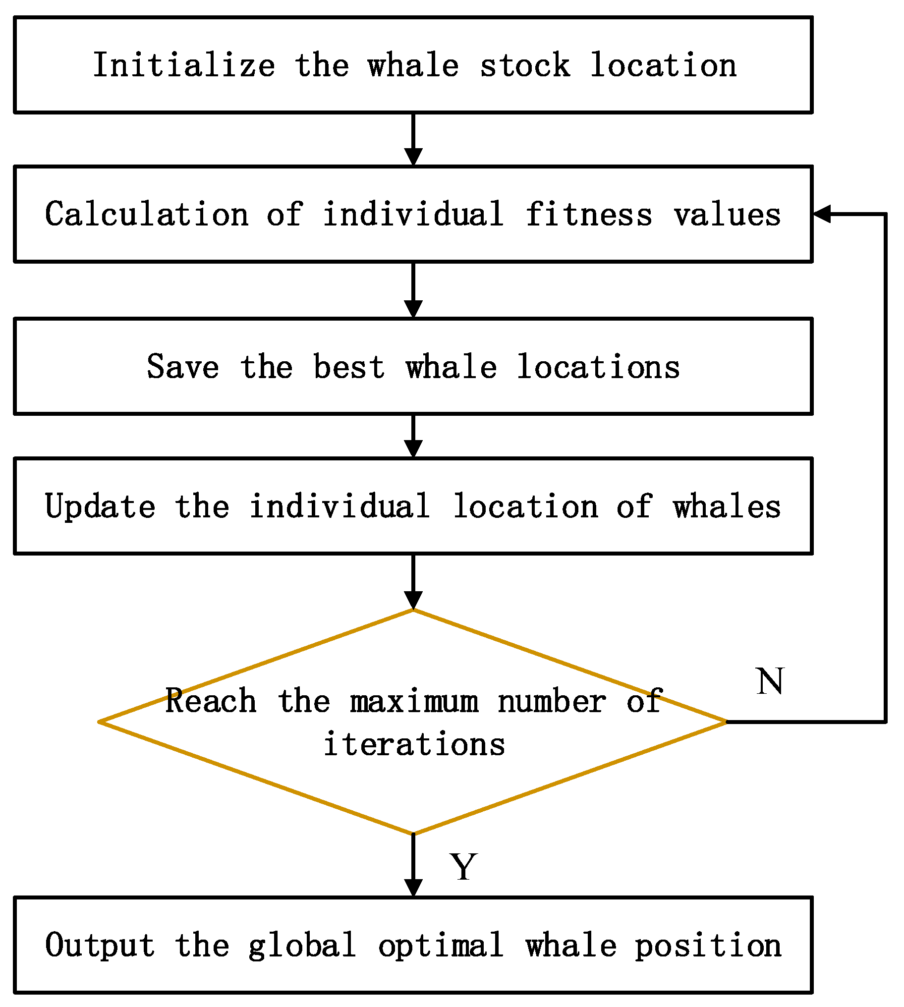
3. Introduction to the WOA

WOA is a novel intelligent meta-inspired optimisation algorithm proposed by Seyedali Mirjalili, an Australian scholar, in 2016. In WOA, the whale prey predation mechanism is simulating [33]. The advantage of WOA is that it better weighs and quantifies the global and local search capabilities. The specific hunting steps are as follows:

(1)

Searching for prey. Whales achieve food hunting by constantly updating their position when searching for prey, as expressed in the following equations:

$$D=\left|C{X}_{\mathrm{rand}}-X\right|$$

(10)

$$X(t+1)=X_{\mathrm{rand}}-AD$$

(11)

where D is the distance between the whale and the prey; t is the number of current iterations; X_rand is the random position vector of the whale; X is the position vector; and A and C are the coefficients.

The coefficients A and C are calculated as follows:

$$A=2ar-a$$

(12)

$$C=2r$$

(13)

where a decreases linearly from 2 to 0, and r is a random value between 0 and 1.

(2)

Surrounding the prey. The whale can identify and cover the location of the prey. Determining the location of the optimal solution in the search space in advance is difficult; therefore, in WOA, the target prey location is assumed to be the initial optimal solution or the closest optimal solution location. When the optimal individual position is determined, other whales try to approach the optimal position and update their positions. The whale encirclement hunting is expressed as follows:

$$D=\left|C{X}^{*}\left(t\right)-X\left(t\right)\right|$$

(14)

$$X(t+1)=X^{*}(t)-AD$$

(15)

where X*(t) is the position of the current optimal solution and is updated in each iteration, and X(t) is the current position vector.

The contraction and encirclement mechanism of whale encircling hunting is displayed in Figure 1, which reveals that the contraction surrounding mechanism continuously narrows the range and accurately surrounds the prey. This method mainly involves decreasing a gradually from 2 to 0.

(3)

Spiral bubble netting for hunting. The whale spiral bubble-net hunting is expressed as follows:

$$X(t+1)=D^{\prime }{e}^{bl}\cos (2\pi l)+X^{*}(t)$$

(16)

$$D^{\prime }=\left|X^{*}\left(t\right)-X\left(t\right)\right|$$

(17)

where $D^{\prime }$ is the distance between the best whale in position and the prey (the current best solution); b is a constant that defines the shape of the spiral; and l is a random value between −1 and 1.

The whale spiral updates the position hunting method, as displayed in Figure 2. As shown in the figure, in the whale spiral bubble-net hunting method, the distance between the best whale in position and the prey is primarily calculated (the current best solution).

The whales were hunted with a 50% probability of choosing each of the aforementioned two hunting methods, as expressed in the following equation:

$$X(t+1)=\{\begin{array}{l}{X}^{*}(t)-AD,\hspace{0.17em}\hspace{0.17em}p\le 0.5\\ D^{\prime }{e}^{bl}\cos (2\pi l)+X^{*}(t),\hspace{0.17em}\hspace{0.17em}p\ge 0.5\end{array}$$

(18)

The range of values of A can be calculated from Equation (12) [–2,2]. WOA exhibits simple operation, mainly adjusting the parameters A and C. By setting A, the WOA exhibits superior exploration and development ability and improves the convergence speed to reach the global optimum. The flowchart of WOA is displayed in Figure 3.

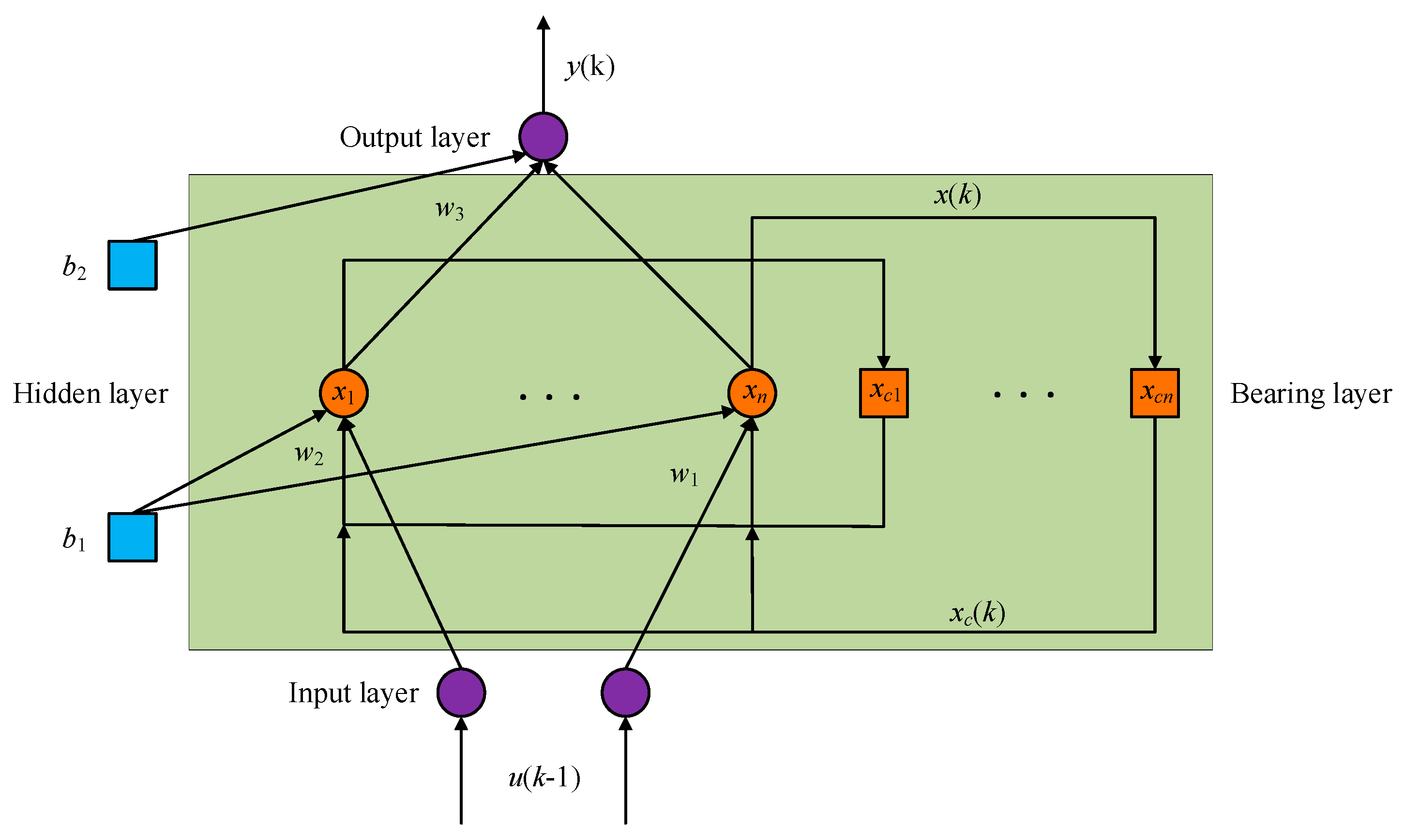
4. Introduction to the Elman Neural Network

4.1. Elman Neural Network Model

The Elman neural network is generally categorised into four layers, namely input, output, implicit, and takeover, as displayed in Figure 4. A unique feature of the Elman neural network is that the output of the implicit layer is self-linked to the input of the implicit layer through the delay and storage of the carryover layer, which renders it sensitive to historical data. Furthermore, the feedback adjustment inside the network enhances the network’s ability to process dynamic information. The commitment layer is equivalent to a delay operator with memory properties, which can satisfactorily solve the static modelling problem and enable the mapping of dynamic systems with the ability to adapt to time-varying characteristics. Thus, the dynamic process characteristics of the system can be directly obtained [34].

The Elman neural network is characterised by the self-linking of the implicit layer output to the implicit layer input through the delay and storage of the association layer. This self-linkage renders the network sensitive to the data of historical states, and the increase in the internal feedback improves the ability of the network itself to process dynamic information to achieve dynamic modelling. The Elman neural network can form temporal and spatial learning patterns through its feedback mechanism, which allows accurate modelling when the mathematical model of the system is unknown and only the input and output of the sample data are given, which can effectively avoid the interference of system data noise on the accuracy of the network calculation results [35].

4.2. Introduction to the Elman Network Algorithm

As displayed in the structure diagram in Figure 4, the nonlinear state-space expression of the Elman neural network is as follows:

$$y(k)=g(w^{3}x(k)+b_2)$$

(19)

$$x(k)=f(w^1{x}_c(k)+w^2(u(k-1))+b_1)$$

(20)

$$x_c(k)=x(k-1)$$

(21)

where k is the moment; y, x, u and x_c are one-dimensional output node vectors, m-dimensional hidden layer node unit vectors, n-dimensional input vectors, and m-dimensional feedback state vectors, respectively; w³, w², and w¹ are the connection weight matrices from the hidden layer to the output layer, the input layer to the hidden layer, and the take-up layer to the hidden layer, respectively; f(·) is the transfer function of the hidden layer neurons; and b₁ and b₂ are the thresholds of the hidden layer and the output layer, respectively.

In the Elman neural network, a gradient descent backpropagation algorithm is used with additional momentum to correct the weight threshold, and the error function E is defined as follows:

$$E=\frac{1}{2}{\displaystyle \sum _{k=1}^n{[y_d(k)-y(k)]}^2}$$

(22)

where y_d(k) is the desired output of the network, and y(k) is the actual output of the network.

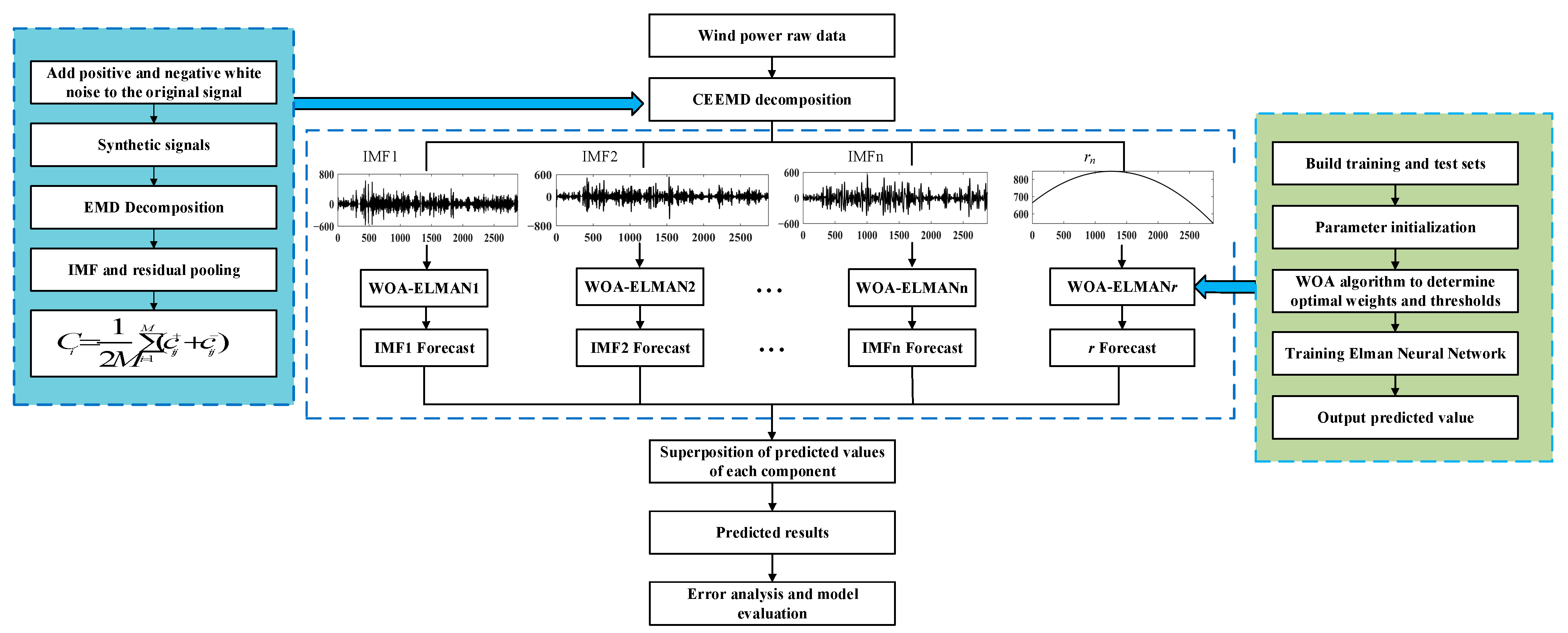
5. Establishment of the CEEMD–WOA–ELMAN Prediction Model

Because of the stochastic fluctuation of the raw wind power time series, achieving high-accuracy wind power prediction by directly using raw power data based on the Elman model is difficult. Therefore, to overcome this challenge, CEEMD is used to decompose the randomly fluctuating raw wind power series into several smoother subseries components, which can not only effectively solve the EMD modal mixing problem but also improve the computational efficiency of the EEMD method with less reconstruction error than EEMD. For the nonlinear unsteady historical wind power series, CEEMD is used to decompose into n IMF components and one residual component.

All components of CEEMD decomposition are categorised into two sets, namely training and test. The training set of each component is used to build the respective Elman model, and the weights and thresholds of the optimised Elman neural network are optimised using the WOA to obtain the prediction model of each component. The test set of each component is used to predict the wind power value at the future moment, and the predicted values of each component are superimposed to obtain the final prediction value and verify the performance of the developed prediction model. In this study, the combined CEEMD–WOA–ELMAN-based ultra-short-term wind power prediction model is constructed as follows:

(1)

The original wind power signal is decomposed using CEEMD to obtain n IMF components and one residual component r_n(t), and a suitable IMF is selected.

(2)

The decomposed IMF components and residual components of the training set are used as the inputs of each component of the Elman wind power model, and the WOA is used to optimise the weights and thresholds of each component of the model to obtain the optimised prediction model of each component.

(3)

In prediction, each IMF component and residual component after decomposition of the test set are inputted into the trained Elman model of each component for prediction, and the predicted values of each component are obtained.

(4)

The predicted values of each component are superimposed to obtain the final wind power prediction at a certain moment.

(5)

Error analysis of the obtained predicted wind power and the actual wind power data is performed.

Figure 5 displays the flowchart of the proposed combined CEEMD–WOA–ELMAN approach.

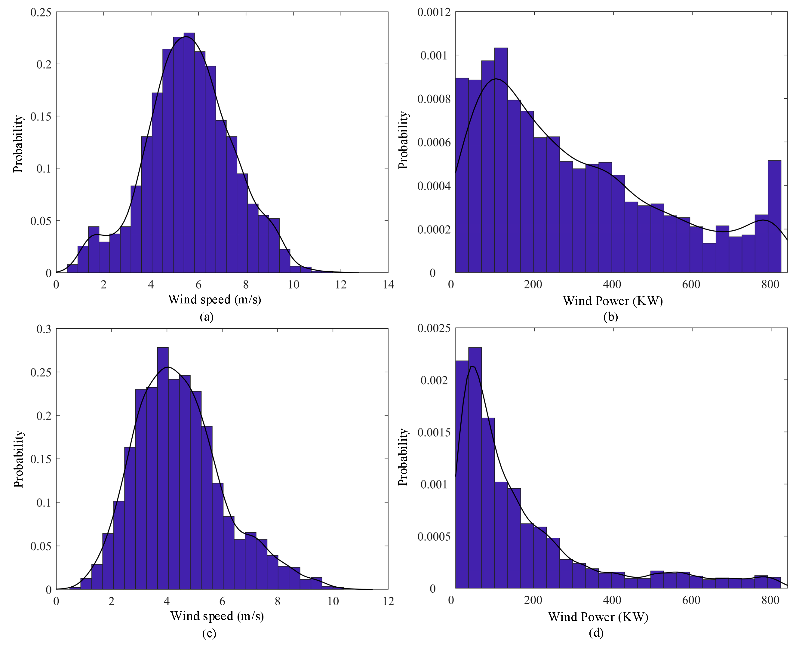
6. Example and Analysis of Results

In this study, the actual operating data of wind turbine No. 2 and wind turbine No. 3 of a wind farm in August 2017 and October 2017, respectively, were used for modelling analysis, with the data sampling time of 15 min and a total of 2880 data points. Figure 6 shows the wind energy probabilities for August No. 2 and October No. 3 wind turbines. As shown in Figure 6a,c, the wind speed range is concentrated in the range of 0–14 m/s, and the wide range of wind speed distribution causes a large fluctuation of power. The power probability diagrams in Figure 6b,d confirm the large fluctuation of power, which is distributed in the range of 0–2000 kW.

Rolling to build the Elman model requires a thorough understanding of the latest change pattern of the wind power system. Therefore, the time window of 10 time points of data is selected; for example, the use of 1–10 points to predict the 11^th point and the use of 2–11 points to predict the 12^th point. A total of 2870 sets of input and output variables are composed; the first 2820 sets are selected as the training sample set, and the next 50 sets are considered the test sample set.

To quantitatively analyse the prediction results and verify the performance of the proposed ultra-short-term wind power portfolio prediction model, root mean square error (RMSE), mean absolute error (MAE), and mean absolute percentage error (MAPE) were calculated. The index of agreement (IA) was proposed by Willmott as a standardized measure of the degree of model prediction error, and its value varies between 0 and 1. A value of 1 indicates a perfect match, whereas a value of 0 indicates no agreement at all. The IA can detect additive and proportional differences in the observed and forecasted means and variances; thus, it can be used to confirm the validity of overperformance [36]. The Pearson correlation coefficient is a linear correlation coefficient that reflects the correlation degree between two variables and is also known as Pearson product-moment correlation coefficient [37]. In this study, the Pearson correlation coefficient is used to determine the correlation between the predicted and actual wind power. $\rho =1$ indicates a completely linear correlation between two variables, Whereas $\rho =0$ indicates a wireless correlation between two variables. The closer the $\rho$ is to 1, the stronger is the linear relationship between two variables. All of these indicators are used to estimate the proposed method. The equations used are as follows:

$$\mathrm{RMSE}=\sqrt{\frac{1}{N}{\displaystyle \sum _{i=1}^N{({\stackrel{⌢}{y}}_i-y_i)}^2}}$$

(23)

$$\mathrm{MAE}=\frac{1}{N}{\displaystyle \sum _{i=1}^N\left|{\stackrel{⌢}{y}}_i-y_i\right|}$$

(24)

$$\mathrm{MAPE}=\frac{1}{N}{\displaystyle \sum _{i=1}^N\left|\frac{{\stackrel{⌢}{y}}_i-y_i}{y_i}\right|}\times 100\%$$

(25)

$$\mathrm{IA}=1-\frac{{\displaystyle \sum _{i=1}^N{({\stackrel{⌢}{y}}_i-y_i)}^2}}{{\displaystyle \sum _{i=1}^N{(\left|{\stackrel{⌢}{y}}_i-\overline{y}\right|+\left|y_i-\overline{y}\right|)}^2}}$$

(26)

$$\rho =\frac{{\displaystyle \sum _{i=1}^N(y_i-\overline{Y})({\stackrel{⌢}{y}}_i-\overline{y})}}{\sqrt{{\displaystyle \sum _{i=1}^N{(y_i-\overline{Y})}^2{\displaystyle \sum _{i=1}^N{({\stackrel{⌢}{y}}_i-\overline{y})}^2}}}}$$

(27)

where n represents the number of test samples, ${\stackrel{⌢}{y}}_i$ is the i-th predicted value, $\overline{y}$ is the mean value of all predicted value, $y_i$ is the i-th true value, and $\overline{Y}$ is the mean value of all true values.

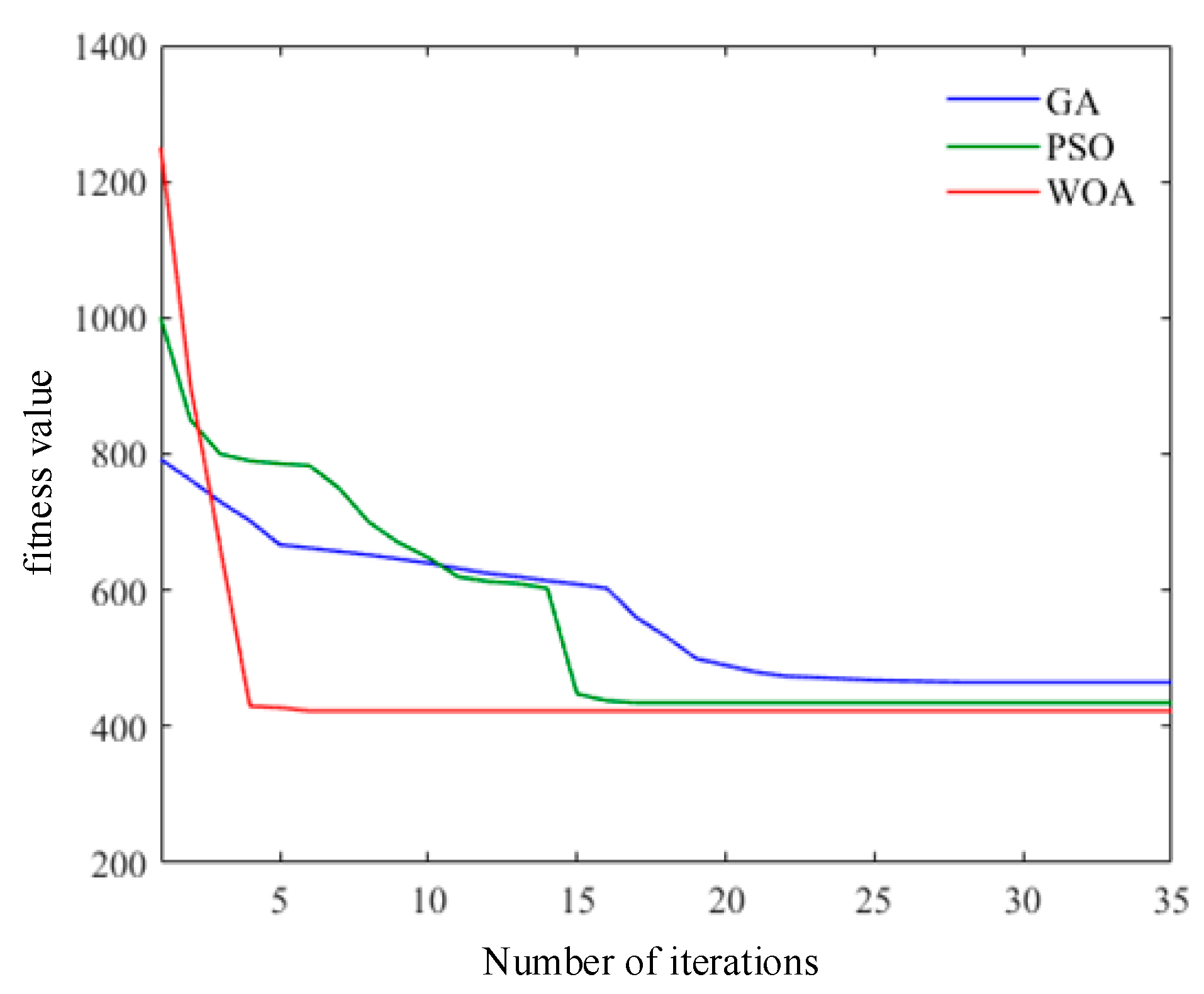
6.1. Optimised Performance Analysis of WOA

To test WOA performance, the WOA was compared with the particle swarm optimisation (PSO) and the genetic algorithm (GA) for the experiment. The iterative change process of the fitness value of each optimisation algorithm is displayed in Figure 7. The initialised population of WOA was 30 and the number of iterations was 35; the initialised population of GA was 30 and the number of iterations was 35; and the initialised population of PSO was 30 and the number of iterations was 35. The fitness function was defined with the average absolute error of training as the criterion. As shown in Figure 6, all three optimisation algorithms decreased rapidly at the beginning of the iteration, and the WOA exhibited the least number of iterations and reached the global optimum convergence in 4 iterations. The GA exhibits a large fitness value when optimising the parameters and requires more than 20 iterations to reach convergence. The PSO can obtain a superior fitness value when eventually optimising the parameters and reaching the global optimum, but it requires approximately 16 iterations to reach stable convergence. Therefore, WOA outperformed the three optimisation algorithms in finding the optimal solution. Through many tests of the optimization model, to obtain the best model performance, the parameter a of WOA decreases linearly from 2 to 0, in which the number of populations is 30 and the number of iterations is 100. Acceleration constants C₁ and C₂ represent the weights of the stochastic acceleration terms that push a particle toward the personal best position and the best positions found by all particles in the swarm, respectively. Regarding PSO, the number of populations is 30, the number of iterations is 100, and the constants C₁ and C₂ are both set to 2. With respect to GA, the number of populations is 30, the number of iterations is 100, the mutation probability is 0.09, and the crossover probability is 0.9.

The advantages and disadvantages of these three optimisation algorithms are examined to optimise the parameters of a single Elman model and predict the power. The prediction effect is compared and analysed in terms of five error evaluation indices, as mentioned in

Table 1. Error evaluation index value of each prediction model under various optimisation algorithms.

Prediction Method	RMSE	MAE	MAPE	IA	$\mathit{\rho }$
GA–ELMAN	35.5133	30.6847	4.8578	0.9646	0.9604
PSO–ELMAN	30.3242	27.4234	4.5706	0.9762	0.9653
WOA–ELMAN	28.4552	25.1618	4.1173	0.9819	0.9726

. The results indicate that in terms of the wind power prediction effect of the Elman model, WOA exhibits smaller prediction error and higher prediction accuracy than GA and PSO.

Figure 8a,b present the statistical results of wind power prediction and prediction error, respectively. The data in the figure reveal that the WOA–ELMAN model outperformed the GA–ELMAN and PSO–ELMAN models. The following conclusions can be drawn: WOA can accurately and effectively search the optimal combination of network connection weights in the training process, avoid the possibility of falling into local minima, and improve model prediction accuracy.

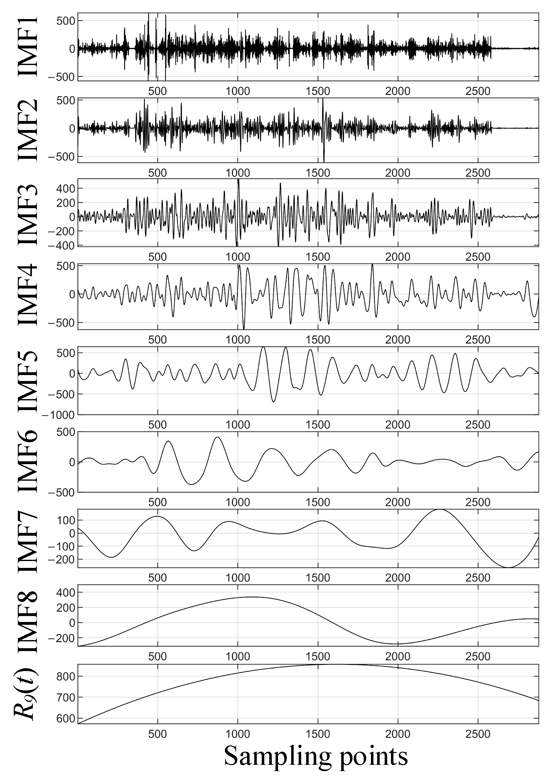
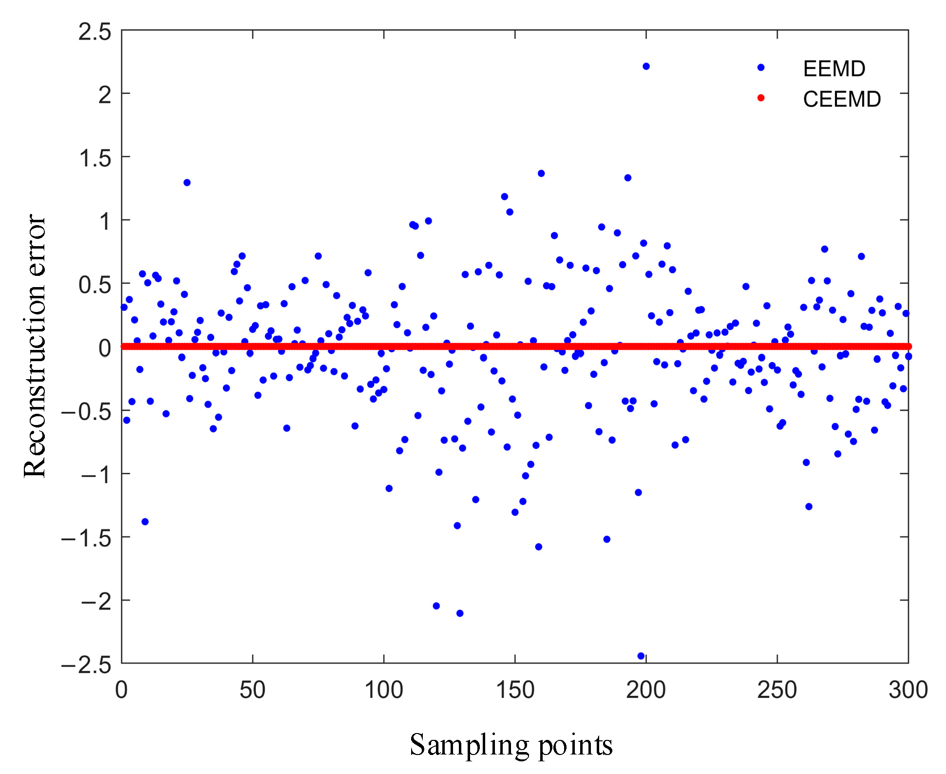
6.2. CEEMD Decomposition of Wind Power Series

The EEMD decomposition and CEEMD decomposition are typically considered to be 0.1 to 0.3 times the standard deviation of the original noise, and the number of white noise added is 100 to 300. Here, both EEMD and CEEMD decompositions are selected to add white noise with a standard deviation of 0.2 and an ensemble number of 200. The wind power data are modally decomposed by CEEMD to avoid slow training of the model and prediction complexity because of over decomposition. Therefore, eight IMF components (IMF1–IMF8) and one residual component are selected in this study, and the decomposition results are displayed in Figure 9.

In this study, the same set of wind power series is decomposed by EEMD and CEEMD, respectively, and the decomposed components are superimposed and reconstructed into a new sequence. As illustrated in Figure 10, the average absolute percentage error MAPE is used to calculate the error between the new sequence and the original sequence, and the reconstruction error of EEMD and CEEMD is finally obtained.

The reconstruction error of EEMD is scattered, whereas the CEEMD error is approximately 0, and their reconstruction errors are $e_{\mathrm{EEMD}}=0.0604\%$ and $e_{\mathrm{CEEMD}}=3.581\times {10}^{-14}\%$ respectively (Figure 10). The experimental results indicate that the reconstruction error of CEEMD is considerably smaller than that of EEMD in the order of magnitude, which is consistent with the theory, thus verifying that CEEMD is superior to EEMD in reducing residual auxiliary noise.

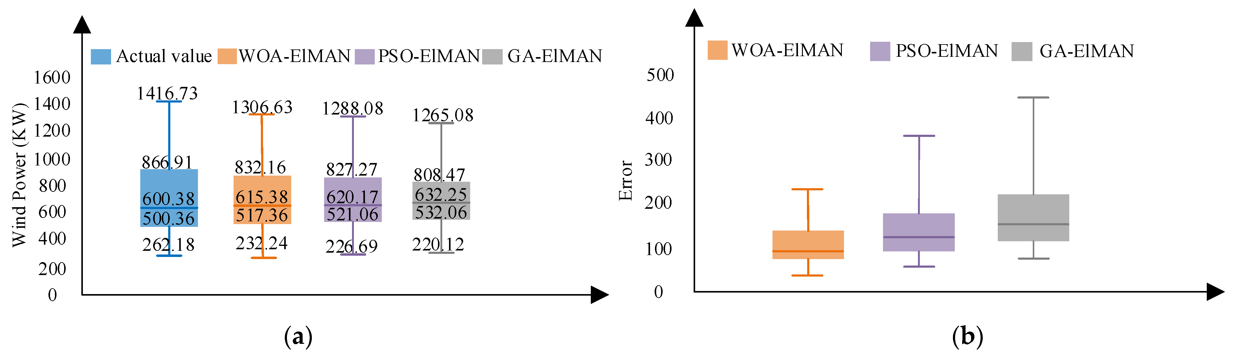
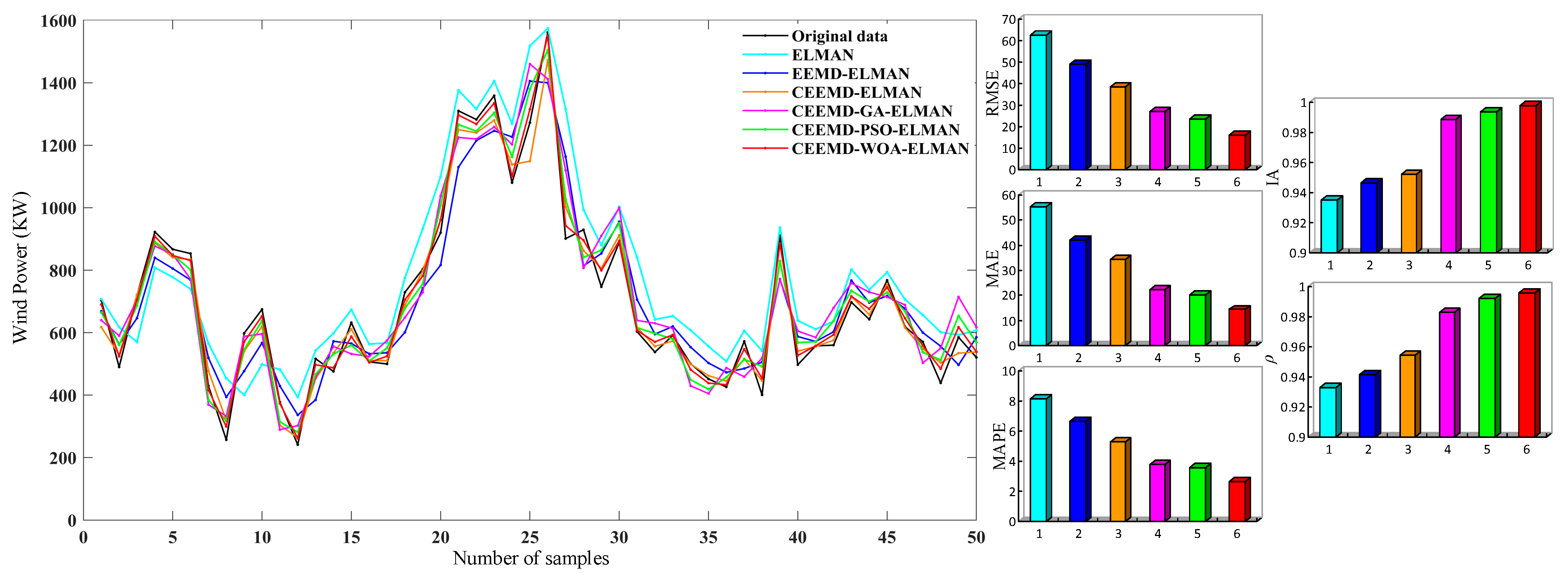
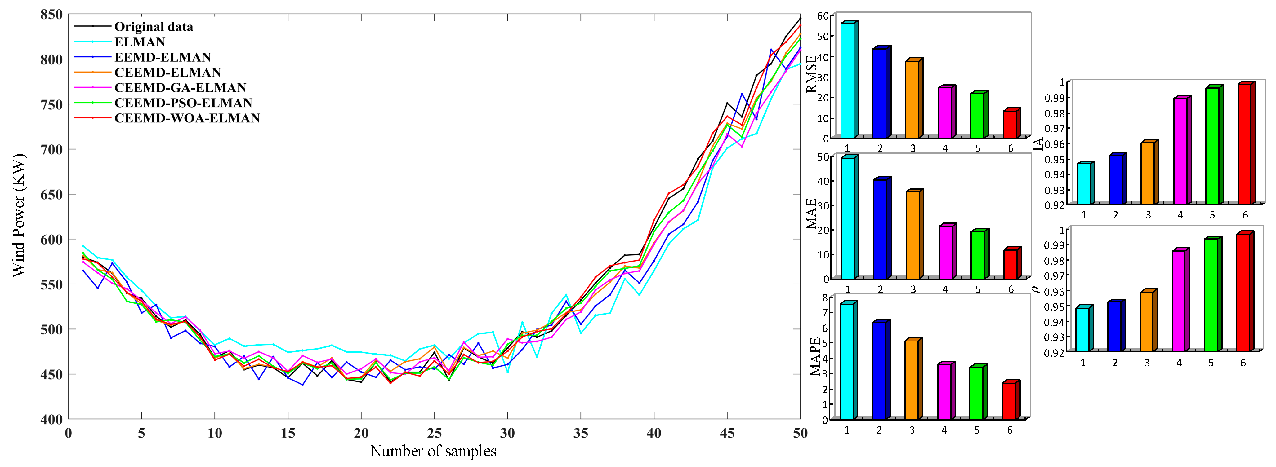
6.3. Ultra-Short-Term Wind Power Prediction Based on CEEMD–WOA–ELMAN

The wind power data are decomposed by CEEMD to obtain eight IMF components and one residual component, and the WOA optimises the weights and thresholds of the nine components and the ELMAN model to finally establish a wind power prediction model based on CEEMD–WOA–ELMAN. To verify the prediction accuracy of the proposed model, wind power ultra-short-term prediction ability for the ELMAN, EEMD–ELMAN, CEEMD–ELMAN, CEEMD–GA–ELMAN, and CEEMD–PSO–ELMAN models are compared; the six wind power prediction results of two wind turbines are displayed in Figure 11 and Figure 12. The results of the six wind power predictions for the two wind turbines are displayed in Figure 11 and Figure 12. Analysis of Figure 11 and Figure 12 indicates that the prediction based on the CEEMD–WOA–ELMAN model exhibits higher precision and accuracy than that based on other models.

To compare the prediction accuracy of the six models, the error analysis of these six models is conducted separately. Error indicators, namely RMSE, MAE, MAPE, IA, and $\rho$, are used to measure the accuracy of wind power prediction, and the prediction results are compared and analysed.

Data in

Table 2. Six model error evaluation indicators for wind turbine No. 2.

Predictive Models	RMSE	MAE	MAPE	IA	$\mathit{\rho }$
ELMAN	62.6313	55.4153	8.1275	0.9352	0.9328
EEMD–ELMAN	48.9622	42.1292	6.6749	0.9464	0.9414
CEEMD–ELMAN	38.3632	34.2585	5.2809	0.9519	0.9542
CEEMD–GA–ELMAN	26.9245	22.2847	3.8168	0.9885	0.9829
CEEMD–PSO–ELMAN	23.6354	20.0438	3.5672	0.9934	0.9921
CEEMD–WOA–ELMAN	16.1332	14.3704	2.6381	0.9978	0.9959

and

Table 3. Six model error evaluation indicators for wind turbine No. 3.

Predictive Models	RMSE	MAE	MAPE	IA	$\mathit{\rho }$
ELMAN	56.1573	49.1307	7.5285	0.9467	0.9485
EEMD–ELMAN	43.5248	40.2365	6.3507	0.9531	0.9523
CEEMD–ELMAN	37.7319	35.5331	5.1657	0.9605	0.9587
CEEMD–GA–ELMAN	24.6524	21.5278	3.6285	0.9892	0.9856
CEEMD–PSO–ELMAN	21.8258	19.3365	3.4536	0.9964	0.9934
CEEMD–WOA–ELMAN	13.2642	11.6409	2.4158	0.9986	0.9967

indicate that the prediction accuracy of each combined model based on EEMD and CEEMD is substantially improved relative to the optimised model Elman without modal decomposition, which indicates that the use of the signal decomposition technique can reduce the volatility of wind power sequences, thereby effectively exploiting the local feature information of the signal and improving prediction performance. The prediction effect of CEEMD is superior to that of EEMD, verifying that CEEMD can solve the problem of large reconstruction errors. The error evaluation indices in Table 2 and Table 3 also show that the combined CEEMD–WOA–ELMAN model exhibits a higher prediction accuracy than CEEMD–GA–ELMAN and CEEMD–PSO–ELMAN by using the same CEEMD decomposition. This result confirms that the WOA exhibits superior optimisation performance for the combined model.

7. Conclusions

As a renewable energy source, wind power can become a major source of electricity generation in China. Therefore, accurate prediction of wind power generation can optimise grid dispatch, reduce system spare capacity, and lower the power system operation cost. An ultra-short-term wind power combination prediction method based on CEEMD–WOA–ELMAN is proposed for wind power time series with strong stochastic fluctuation characteristics. The conclusions are as follows:

(1)

The CEEMD technique can effectively avoid the defect of EEMD with large residual auxiliary noise. In this study, for the CEEMD decomposition of ultra-short-term wind power, a suitable number of IMF components were selected to reduce the complexity of the prediction process.

(2)

In this study, we introduce the WOA with a strong optimising ability to optimise the weights and thresholds of the Elman model, which improves the accuracy of wind power prediction considerably.

(3)

By comparing the WOA with the GA and PSO, we find that the WOA exhibits a fast convergence speed and can effectively avoid falling into local extremes to achieve the optimal effect.

(4)

The actual operating data of two wind turbines in a wind farm are analysed for model performance verification, which indicates that the CEEMD method can obtain smoother IMF components, and the CEEMD–WOA–ELMAN model can achieve superior wind power prediction, further verifying the superiority of the proposed model for achieving excellent wind power prediction.

(5)

The proposed method in this study is better in predicting trend following and prediction accuracy and is suitable for predicting wind power time series with high volatility and strong nonlinearity. Although the proposed method performs well, 15 min is selected as the prediction interval in this study, and different time scales may have different impact results. In the future, the effects of various time scales on ultra-short-term wind power prediction should be analysed, and the model should be optimised to reduce the running time and improve model accuracy.

References

1. Lujano-Rojas, J.; Osório, G.; Matias, J.; Catalão, J. A heuristic methodology to economic dispatch problem incorporating renewable power forecasting error and system reliability. Renew. Energy 2016, 87, 731–743. [Google Scholar] [CrossRef]
2. Carta, J.A.; Velázquez, S.; Cabrera, P. A review of measure-correlate-predict (MCP) methods used to estimate long-term wind characteristics at a target site. Renew. Sust. Energy. Rev. 2013, 27, 362–400. [Google Scholar] [CrossRef]
3. Tascikaraoglu, A.; Uzunoglu, M. A review of combined approaches for prediction of short-term wind speed and power. Renew. Sust. Energy Rev. 2014, 34, 243–254. [Google Scholar] [CrossRef]
4. Sarwat, A.I.; Amini, M.; Domijan, A.; Damnjanovic, A.; Kaleem, F. Weather-based interruption prediction in the smart grid utilizing chronological data. J. Mod. Power Syst. Clean Energy 2016, 4, 1–8. [Google Scholar] [CrossRef] [Green Version]
5. Liu, H.; Mi, X.; Li, Y. Wind speed forecasting method based on deep learning strategy using empirical wavelet transform, long short term memory neural network and Elman neural network. Energy Convers. Manag. 2018, 156, 498–514. [Google Scholar] [CrossRef]
6. Khosravi, A.; Machado, L.; Nunes, R. Time-series prediction of wind speed using machine learning algorithms: A case study Osorio wind farm, Brazil. Appl. Energy 2018, 224, 550–566. [Google Scholar] [CrossRef]
7. Liu, Y.; Guan, L.; Hou, C.; Han, H.; Liu, Z.; Sun, Y.; Zheng, M. Wind power short-term prediction based on LSTM and discrete wavelet transform. Appl. Sci. 2019, 9, 1108. [Google Scholar] [CrossRef] [Green Version]
8. Li, L.; Liu, Y.; Yang, Y.; Han, S.; Wang, Y. A physical approach of the short-term wind power prediction based on CFD pre-calculated flow fields. J. Hydrodyn. Ser. B 2013, 25, 56–61. [Google Scholar] [CrossRef]
9. Okumus, I.; Dinler, A. Current status of wind energy forecasting and a hybrid method for hourly predictions. Energy Convers. Manag. 2016, 123, 362–371. [Google Scholar] [CrossRef]
10. Papaefthymiou, G.; Klockl, B. MCMC for wind power simulation. IEEE Trans. Energy Convers. 2008, 23, 234–240. [Google Scholar] [CrossRef] [Green Version]
11. Taylor, J.W.; McSharry, P.E.; Buizza, R. Wind power density forecasting using ensemble predictions and time series models. IEEE Trans. Energy Convers. 2009, 24, 775–782. [Google Scholar] [CrossRef]
12. Heinermann, J.; Kramer, O. Machine learning ensembles for wind power prediction. Renew. Energy 2016, 89, 671–679. [Google Scholar] [CrossRef]
13. Arshad, J.; Zameer, A.; Khan, A. Wind power prediction using genetic programming based ensemble of artificial neural networks (GPeANN). In Proceedings of the 2014 12th International Conference on Frontiers of Information Technology, Islamabad, Pakistan, 17–19 December 2014. [Google Scholar]
14. Wang, C.; Zhang, H.; Fan, W.; Ma, P. A new chaotic time series hybrid prediction method of wind power based on EEMD-SE and full-parameters continued fraction. Energy 2017, 138, 977–990. [Google Scholar] [CrossRef]
15. Huang, C.Y. Analysis on Application of Wavelet Neural Network in Wind Electricity Power Prediction. Appl. Mech. Mater. 2014, 686, 627–633. [Google Scholar] [CrossRef]
16. De Aquino, R.R.; Neto, O.N.; Souza, R.B.; Lira, M.M.; Carvalho, M.A.; Ludermir, T.B.; Ferreira, A.A. Investigating the use of echo state networks for prediction of wind power generation. In Proceedings of the 2014 IEEE Symposium on Computational Intelligence for Engineering Solutions (CIES), Orlando, FL, USA, 9–12 December 2014. [Google Scholar]
17. Fang, B.; Liu, D.; Wang, B.; Yan, B.; Wang, X. Forecast of Short-term Wind Speed Based on Wavelet Transform and Improved Firefly LSSVM Algorithm. Prot. Control Power Syst. 2016, 44, 37–43. [Google Scholar]
18. Kurbatskii, V.G.; Sidorov, D.N.; Spiryaev, V.A.; Tomin, N.V. On the neural network approach for forecasting of nonstationary time series on the basis of the Hilbert-Huang transform. Autom. Remote Control 2011, 72, 1405–1414. [Google Scholar] [CrossRef]
19. Lv, S.X.; Wang, L. Deep learning combined wind speed forecasting with hybrid time series decomposition and multi-objective parameter optimization. Appl. Energy 2022, 311, 118674. [Google Scholar] [CrossRef]
20. Wang, J.; Wang, S.; Zeng, B.; Lu, H. A novel ensemble probabilistic forecasting system for uncertainty in wind speed. Appl. Energy 2022, 313, 118796. [Google Scholar] [CrossRef]
21. Zhang, G.; Wu, Y.; Wong, K.P.; Xu, Z.; Dong, Z.Y.; Iu, H.-C. An advanced approach for construction of optimal wind power pre-diction intervals. IEEE Trans. Power Syst. 2015, 30, 2706–2715. [Google Scholar] [CrossRef]
22. Yu, C.; Li, Y.; Zhang, M. Comparative study on three new hybrid models using Elman Neural Network and Empirical Mode Decomposition based technologies improved by Singular Spectrum Analysis for hour-ahead wind speed forecasting. Energy Convers. Manag. 2017, 147, 75–85. [Google Scholar] [CrossRef]
23. Su, Y.; Wang, S.; Xiao, Z.; Tan, M.; Wang, M. An ultra-short-term wind power forecasting approach based on wind speed decomposition, wind direction and elman neural networks. In Proceedings of the 2018 2nd IEEE Conference on Energy Internet and Energy System Integration (EI2), Beijing, China, 20–22 October 2018. [Google Scholar]
24. Wang, K.; Niu, D.; Sun, L.; Zhen, H.; Liu, J.; De, G.; Xu, X. Wind power short-term forecasting hybrid model based on CEEMD-SE method. Processes 2019, 7, 843. [Google Scholar] [CrossRef] [Green Version]
25. Sun, Z.; Liu, Y.; Xu, M.; Guan, W. Wind power prediction based on Elman neural network model optimized by improved genetic algorithm. In Proceedings of the 2021 IEEE 2nd International Conference on Big Data, Artificial Intelligence and Internet of Things Engineering (ICBAIE), Nanchang, China, 26–28 March 2021. [Google Scholar]
26. Xie, K.; Yi, H.; Hu, G.; Li, L.; Fan, Z. Short-term power load forecasting based on Elman neural network with particle swarm optimization. Neurocomputing 2020, 416, 136–142. [Google Scholar] [CrossRef]
27. Osama, S.; Houssein, E.H.; Hassanien, A.E.; Fahmy, A.A. Forecast of wind speed based on whale optimization algorithm. In Proceedings of the Proceedings of the 1st International Conference on Internet of Things and Machine Learning, Liverpool, UK, 17–18 October 2017. [Google Scholar]
28. Wang, H.; Lv, X.; Luo, X. Short-term Load Forecasting of Power grid Based on Improved WOA Optimized LSTM. In Proceedings of the 2020 5th International Conference on Power and Renewable Energy (ICPRE), Shanghai, China, 12–14 September 2020. [Google Scholar]
29. Huang, N.E.; Shen, Z.; Long, S.R.; Wu, M.C.; Shih, H.H.; Zheng, Q.; Yen, N.-C.; Tung, C.C.; Liu, H.H. The empirical mode decomposition and the Hilbert spectrum for nonlinear and non-stationary time series analysis. Proc. R. Soc. Lond. Ser. A 1998, 454, 903–995. [Google Scholar] [CrossRef]
30. Wu, Z.; Huang, N.E. Ensemble empirical mode decomposition: A noise-assisted data analysis method. Adv. Adapt. Data Anal. 2009, 1, 1–41. [Google Scholar] [CrossRef]
31. Wang, J.; Zhang, W.; Li, Y.; Wang, J.; Dang, Z. Forecasting wind speed using empirical mode decomposition and Elman neural network. Appl. Soft Comput. 2014, 23, 452–459. [Google Scholar] [CrossRef]
32. Yeh, J.R.; Shieh, J.S.; Huang, N.E. Complementary ensemble empirical mode decomposition: A novel noise enhanced data analysis method. Adv. Adapt. Data Anal. 2010, 2, 135–156. [Google Scholar] [CrossRef]
33. Mirjalili, S.; Lewis, A. The whale optimization algorithm. Adv. Eng. Softw. 2016, 95, 51–67. [Google Scholar] [CrossRef]
34. Elman, J.L. Finding structure in time. Cogn Sci. 1990, 14, 179–211. [Google Scholar] [CrossRef]
35. Zhang, X.; Wang, R.; Liao, T.; Zhang, T.; Zha, Y. Short-term forecasting of wind power generation based on the similar day and Elman neural network. In Proceedings of the 2015 IEEE Symposium Series on Computational Intelligence, Cape Town, South Africa, 7–10 December 2015. [Google Scholar]
36. Osório, G.J.; Matias, J.C.O.; Catalão, J.P.S. Short-term wind power forecasting using adaptive neuro-fuzzy inference system combined with evolutionary particle swarm optimization, wavelet transform and mutual information. Renew. Energy 2015, 75, 301–307. [Google Scholar] [CrossRef]
37. Jiang, Z.; Che, J.; Wang, L. Ultra-short-term wind speed forecasting based on EMD-VAR model and spatial correlation. Energy Convers. Manag. 2021, 250, 114919. [Google Scholar] [CrossRef]
Figure 1. Shrink surround mechanism surrounds hunting.
Energies 15 03055 g001
Figure 2. Spiral bubble netting for hunting.
Energies 15 03055 g002
Figure 3. WOA flowchart.
Energies 15 03055 g003
Figure 4. Elman network structure.
Energies 15 03055 g004
Figure 5. Flowchart based on the combined CEEMD–WOA–ELMAN method.
Energies 15 03055 g005
Figure 6. Wind Energy Probability Chart. (a) Wind speed probability distribution of wind turbine No. 2, (b) Power probability distribution of wind turbine No. 2, (c) Wind speed probability distribution of wind turbine No. 3, (d) Power probability distribution of wind turbine No. 3.
Energies 15 03055 g006
Figure 7. Fitness curve of algorithm optimisation parameters.
Energies 15 03055 g007
Figure 8. Comparison of statistical results of predicted values. Statistical results of (a) wind power prediction and (b) prediction error.
Energies 15 03055 g008
Figure 9. Wind power data CEEMD decomposition results.
Energies 15 03055 g009
Figure 10. Reconstruction error of EEMD and CEEMD.
Energies 15 03055 g010
Figure 11. Wind power prediction results of six models of Number Two wind turbine.
Energies 15 03055 g011
Figure 12. Wind power prediction results of six models of Number Three wind turbine.
Energies 15 03055 g012