
Thermoelectric Generator as the Waste Heat Recovery Unit of Proton Exchange Membrane Fuel Cell: A Numerical Study


Abstract
:1. Introduction
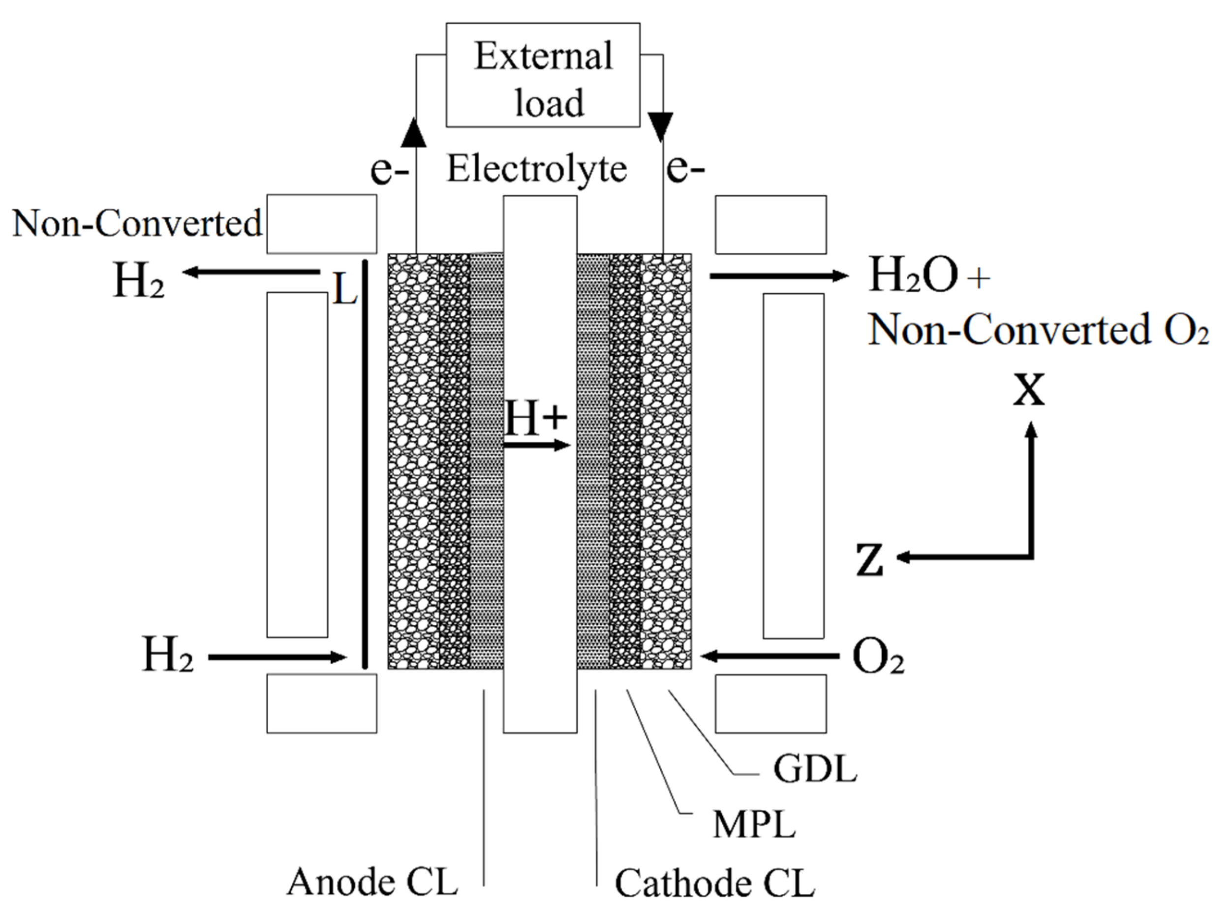
2. Problem Description and Governing Equations
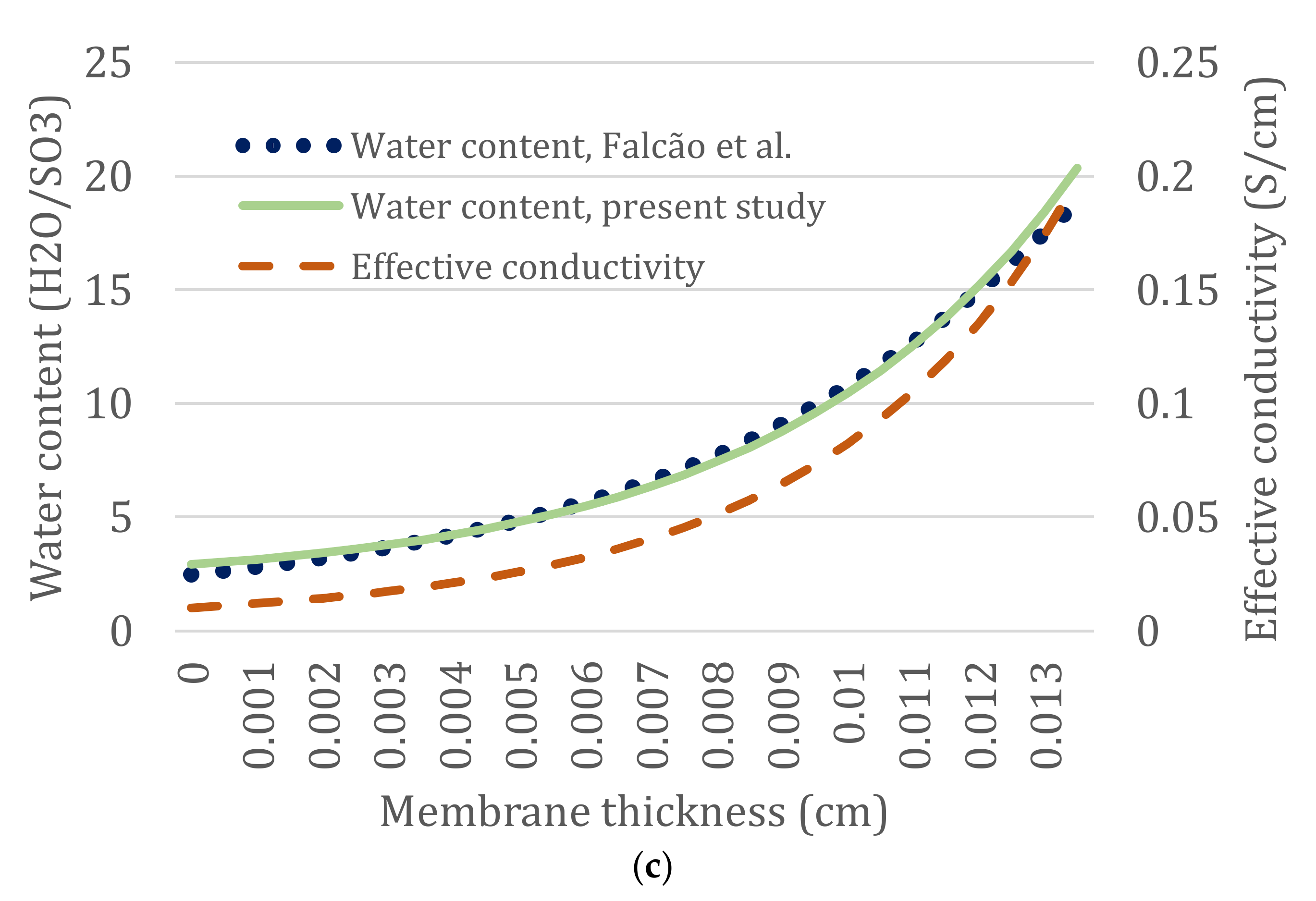
2.1. Membrane
2.2. Catalyst Layer
2.3. Thermoelectric Generator (TEG)
3. Results and Discussion
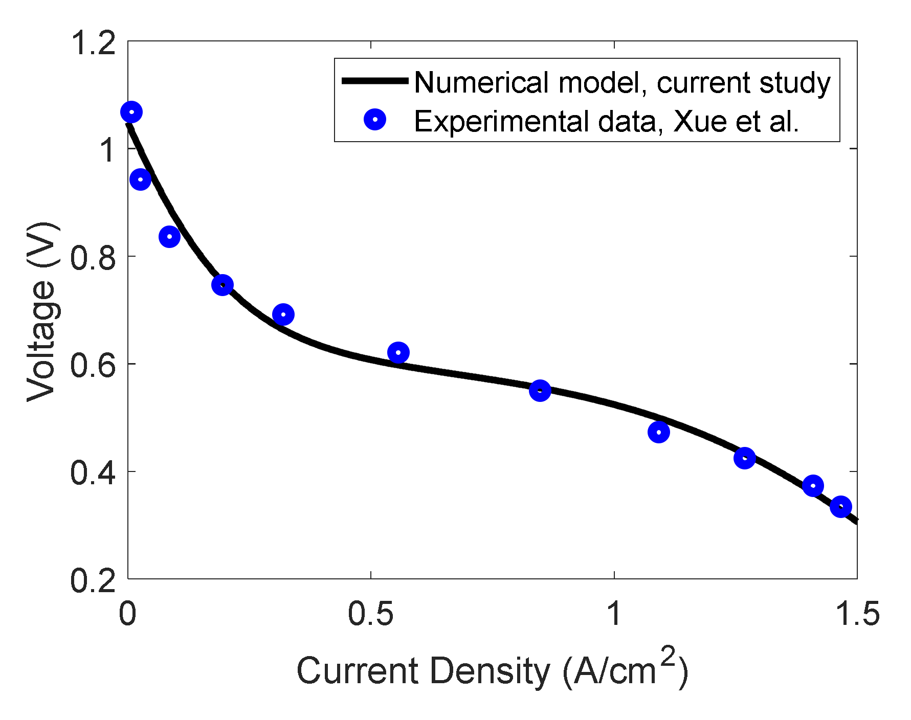
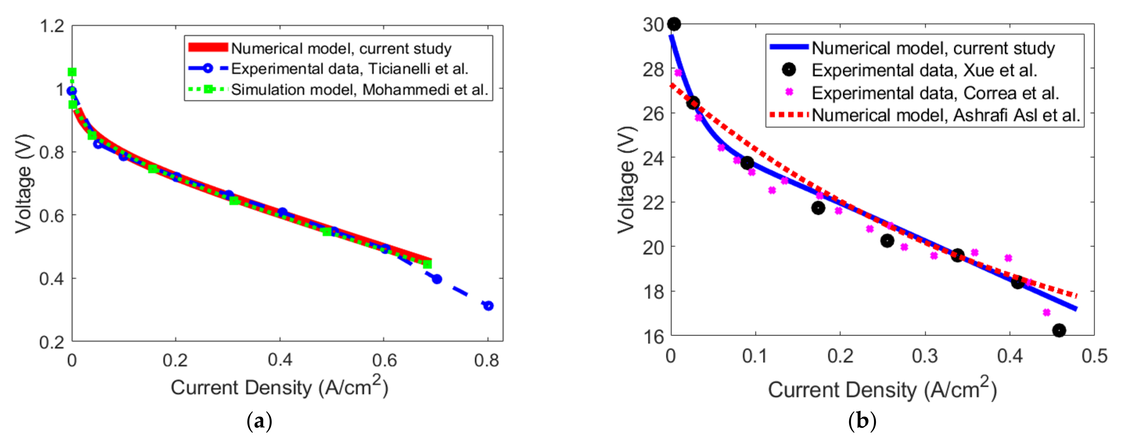
3.1. Model Validation
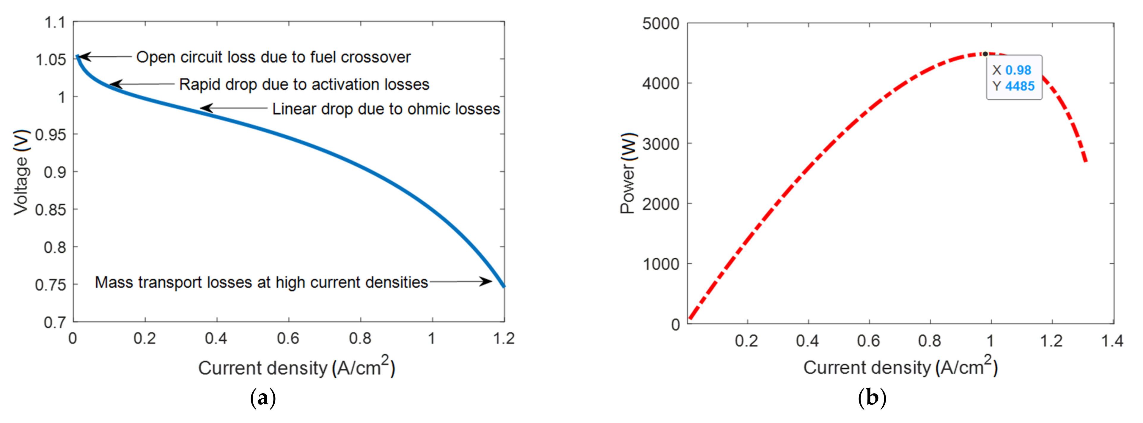
3.2. PEMFC Modeling
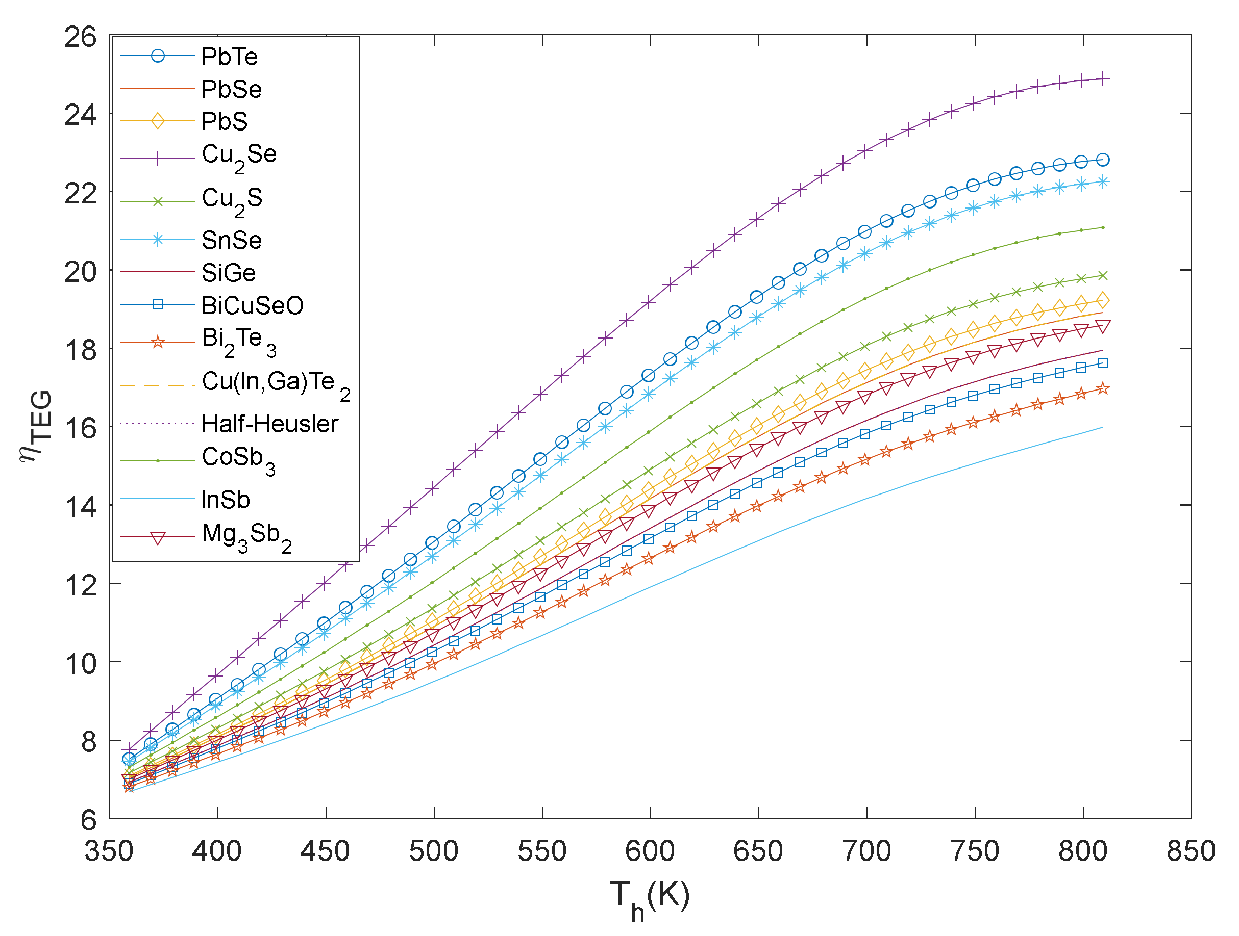
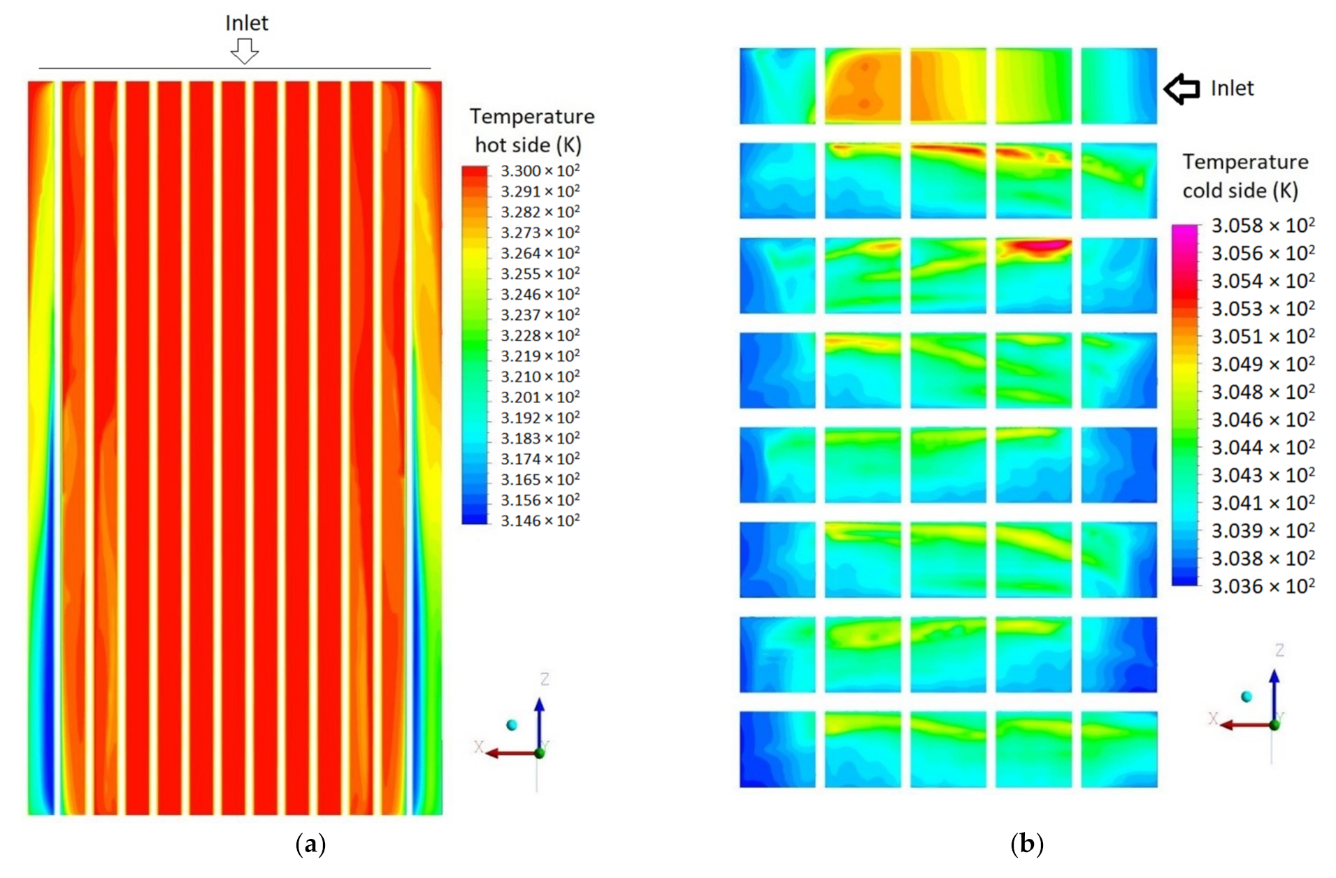
3.3. TEG Simulation
4. Conclusions
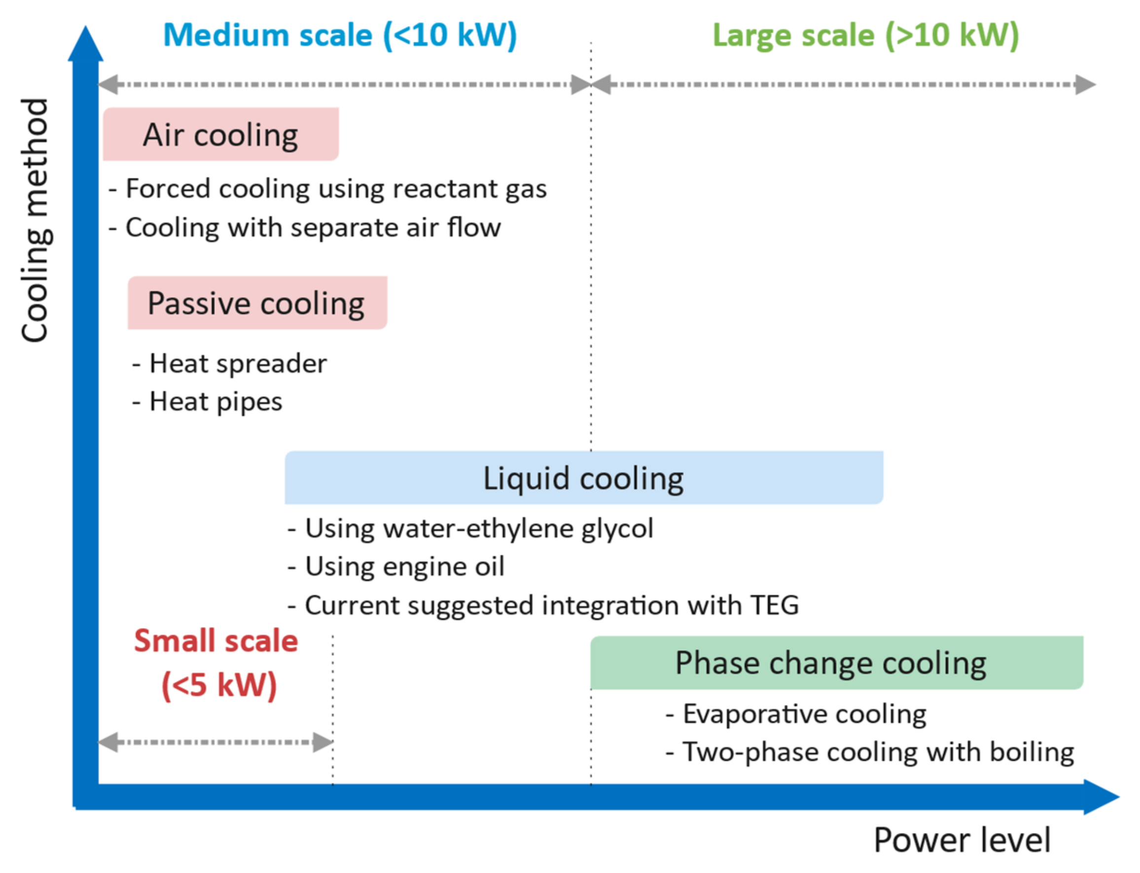
- This study only evaluated the possibility of using a TEG unit as a cooling method in a medium-scale PEMFC stack by calculating the output power and the voltage of the TEG unit. However, exergy and economic aspects of the system could be assessed through exergo-economic and thermo-economic analyses to evaluate the suitability of this integration.
- The design of the current TEG unit was inspired from the geometry given in ref. [28], which was mainly for diesel engine applications. Due to the novelty of this topic, there is a lack of optimized geometry for the application of PEMFC. In this regard, further studies on the geometry of the TEG unit, the needed number of TEG modules in the TEG unit, and the required mechanical/physical properties of the unit for maximum performance are needed.
- The current modeling was performed in the steady-state condition for both the PEMFC numerical model and the TEG simulation model. However, performing a dynamic and real-time analysis would be of value to better investigate the possibility of the current integration.
- The materials in the TEG modules and their figures of merit play a crucial role in the performance of the TEG unit and the waste heat recovery. This study assumed as the base material of the TEG modules, while many other alternatives can be analyzed and evaluated to reach the highest waste heat recovery.
Author Contributions
Funding
Data Availability Statement
Acknowledgments
Conflicts of Interest
References
- Farias, C.B.; Barreiros, R.C.; da Silva, M.F.; Casazza, A.A.; Converti, A.; Sarubbo, L.A. Use of Hydrogen as Fuel: A Trend of the 21st Century. Energies 2022, 15, 311. [Google Scholar] [CrossRef]
- Shahabuddin, M.; Mofijur, M.; Shuvho, M.; Ahmed, B.; Chowdhury, M.A.K.; Kalam, M.A.; Masjuki, H.H.; Chowdhury, M.A. A Study on the Corrosion Characteristics of Internal Combustion Engine Materials in Second-Generation Jatropha Curcas Biodiesel. Energies 2021, 14, 4352. [Google Scholar] [CrossRef]
- Luciani, S.; Tonoli, A. Control Strategy Assessment for Improving PEM Fuel Cell System Efficiency in Fuel Cell Hybrid Vehicles. Energies 2022, 15, 2004. [Google Scholar] [CrossRef]
- Choi, J.; Sim, J.; Oh, H.; Min, K. Resistance Separation of Polymer Electrolyte Membrane Fuel Cell by Polarization Curve and Electrochemical Impedance Spectroscopy. Energies 2021, 14, 1491. [Google Scholar] [CrossRef]
- Cigolotti, V.; Genovese, M.; Fragiacomo, P. Comprehensive Review on Fuel Cell Technology for Stationary Applications as Sustainable and Efficient Poly-Generation Energy Systems. Energies 2021, 14, 4963. [Google Scholar] [CrossRef]
- Nguyen, H.L.; Han, J.; Nguyen, X.L.; Yu, S.; Goo, Y.-M.; Le, D.D. Review of the Durability of Polymer Electrolyte Membrane Fuel Cell in Long-Term Operation: Main Influencing Parameters and Testing Protocols. Energies 2021, 14, 4048. [Google Scholar] [CrossRef]
- Nishimura, A.; Toyoda, K.; Kojima, Y.; Ito, S.; Hu, E. Numerical Simulation on Impacts of Thickness of Nafion Series Membranes and Relative Humidity on PEMFC Operated at 363 K and 373 K. Energies 2021, 14, 8256. [Google Scholar] [CrossRef]
- Mariani, M.; Peressut, A.B.; Latorrata, S.; Balzarotti, R.; Sansotera, M.; Dotelli, G. The Role of Fluorinated Polymers in the Water Management of Proton Exchange Membrane Fuel Cells: A Review. Energies 2021, 14, 8387. [Google Scholar] [CrossRef]
- Rashidi, S.; Karimi, N.; Sunden, B.; Kim, K.C.; Olabi, A.G.; Mahian, O. Progress and challenges on the thermal management of electrochemical energy conversion and storage technologies: Fuel cells, electrolysers, and supercapacitors. Prog. Energy Combust. Sci. 2022, 88, 100966. [Google Scholar] [CrossRef]
- Hmad, A.A.; Dukhan, N. Cooling Design for PEM Fuel-Cell Stacks Employing Air and Metal Foam: Simulation and Experiment. Energies 2021, 14, 2687. [Google Scholar] [CrossRef]
- Woolley, E.; Luo, Y.; Simeone, A. Industrial waste heat recovery: A systematic approach. Sustain. Energy Technol. Assess. 2018, 29, 50–59. [Google Scholar] [CrossRef]
- Nishimura, A.; Kojima, Y.; Ito, S.; Hu, E. Impacts of Separator Thickness on Temperature Distribution and Power Generation Characteristics of a Single PEMFC Operated at Higher Temperature of 363 and 373 K. Energies 2022, 15, 1558. [Google Scholar] [CrossRef]
- Blanco-Cocom, L.; Botello-Rionda, S.; Ordoñez, L.C.; Valdez, S.I. A Self-Validating Method via the Unification of Multiple Models for Consistent Parameter Identification in PEM Fuel Cells. Energies 2022, 15, 885. [Google Scholar] [CrossRef]
- Kravos, A.; Kregar, A.; Mayer, K.; Hacker, V.; Katrašnik, T. Identifiability Analysis of Degradation Model Parameters from Transient CO2 Release in Low-Temperature PEM Fuel Cell under Various AST Protocols. Energies 2021, 14, 4380. [Google Scholar] [CrossRef]
- Zhang, G.; Jiao, K. Multi-phase models for water and thermal management of proton exchange membrane fuel cell: A review. J. Power Sources 2018, 391, 120–133. [Google Scholar] [CrossRef]
- Mu, Y.-T.; He, P.; Gu, Z.-L.; Qu, Z.-G.; Tao, W.-Q. Modelling the reactive transport processes in different reconstructed agglomerates of a PEFC catalyst layer. Electrochim. Acta 2022, 404, 139721. [Google Scholar] [CrossRef]
- Pourrahmani, H.; Siavashi, M.; Moghimi, M. Design optimization and thermal management of the PEMFC using artificial neural networks. Energy 2019, 182, 443–459. [Google Scholar] [CrossRef]
- Pourrahmani, H.; Moghimi, M.; Siavashi, M.; Shirbani, M. Sensitivity analysis and performance evaluation of the PEMFC using wave-like porous ribs. Appl. Therm. Eng. 2019, 150, 433–444. [Google Scholar] [CrossRef]
- Pourrahmani, H.; Moghimi, M.; Siavashi, M. Thermal management in PEMFCs: The respective effects of porous media in the gas flow channel. Int. J. Hydrogen Energy 2019, 44, 3121–3137. [Google Scholar] [CrossRef]
- Kwan, T.H.; Wu, X.; Yao, Q. Bidirectional operation of the thermoelectric device for active temperature control of fuel cells. Appl. Energy 2018, 222, 410–422. [Google Scholar] [CrossRef] [Green Version]
- Kwan, T.H.; Wu, X.; Yao, Q. Multi-objective genetic optimization of the thermoelectric system for thermal management of proton exchange membrane fuel cells. Appl. Energy 2018, 217, 314–327. [Google Scholar] [CrossRef]
- Kwan, T.H.; Shen, Y.; Yao, Q. An energy management strategy for supplying combined heat and power by the fuel cell thermoelectric hybrid system. Appl. Energy 2019, 251, 113318. [Google Scholar] [CrossRef]
- Shen, Y.; Kwan, T.H.; Yao, Q. Performance numerical analysis of thermoelectric generator sizing for integration into a high temperature proton exchange membrane fuel cell. Appl. Therm. Eng. 2020, 178, 115486. [Google Scholar] [CrossRef]
- Shen, Y.; Zhao, B.; Kwan, T.H.; Yao, Q. Numerical analysis of combined air-cooled fuel cell waste heat and thermoelectric heating method for enhanced water heating. Energy Convers. Manag. 2020, 213, 112840. [Google Scholar] [CrossRef]
- Tuoi, T.T.K.; Toan, N.V.; Ono, T. Theoretical and experimental investigation of a thermoelectric generator (TEG) integrated with a phase change material (PCM) for harvesting energy from ambient temperature changes. Energy Rep. 2020, 6, 2022–2029. [Google Scholar] [CrossRef]
- He, J.; Tritt, T.M. Advances in thermoelectric materials research: Looking back and moving forward. Science 2017, 357, eaak9997. [Google Scholar] [CrossRef] [PubMed] [Green Version]
- Jouhara, H.; Żabnieńska-Góra, A.; Khordehgah, N.; Doraghi, Q.; Ahmad, L.; Norman, L.; Axcell, B.; Wrobel, L.; Dai, S. Thermoelectric generator (TEG) technologies and applications. Int. J. Thermofluids 2021, 9, 100063. [Google Scholar] [CrossRef]
- Fernández-Yañez, P.; Armas, O.; Capetillo, A.; Martínez-Martínez, S. Thermal analysis of a thermoelectric generator for light-duty diesel engines. Appl. Energy 2018, 226, 690–702. [Google Scholar] [CrossRef]
- Zorbas, K.T.; Hatzikraniotis, E.; Paraskevopoulos, K.M. Power and Efficiency Calculation in Commercial TEG and Application in Wasted Heat Recovery in Automobile. In Proceedings of the 5th European Conference on Thermoelectrics, Odessa, Ukraine, 10–12 September 2007; p. 4. [Google Scholar]
- Arasteh, H.; Mashayekhi, R.; Ghaneifar, M.; Toghraie, D.; Afrand, M. Heat transfer enhancement in a counter-flow sinusoidal parallel-plate heat exchanger partially filled with porous media using metal foam in the channels’ divergent sections. J. Therm. Anal. Calorim. 2020, 141, 1669–1685. [Google Scholar] [CrossRef]
- Spiegel, C. PEM Fuel Cell Modeling and Simulation Using Matlab; Academic Press: Cambridge, MA, USA; Elsevier: Amsterdam, The Netherlands, 2008. [Google Scholar]
- Li, S.; Yuan, J.; Xie, G.; Sundén, B. Effects of agglomerate model parameters on transport characterization and performance of PEM fuel cells. Int. J. Hydrogen Energy 2018, 43, 8451–8463. [Google Scholar] [CrossRef] [Green Version]
- Thosar, A.U.; Agarwal, H.; Govarthan, S.; Lele, A.K. Comprehensive analytical model for polarization curve of a PEM fuel cell and experimental validation. Chem. Eng. Sci. 2019, 206, 96–117. [Google Scholar] [CrossRef]
- Siegel, N.P.; Ellis, M.W.; Nelson, D.J.; von Spakovsky, M.R. A two-dimensional computational model of a PEMFC with liquid water transport. J. Power Sources 2004, 128, 173–184. [Google Scholar] [CrossRef]
- Ge, M.; Zhao, Y.; Li, Y.; He, W.; Xie, L.; Zhao, Y. Structural optimization of thermoelectric modules in a concentration photovoltaic–thermoelectric hybrid system. Energy 2022, 244, 123202. [Google Scholar] [CrossRef]
- Ge, M.; Li, Z.; Wang, Y.; Zhao, Y.; Zhu, Y.; Wang, S.; Liu, L. Experimental study on thermoelectric power generation based on cryogenic liquid cold energy. Energy 2021, 220, 119746. [Google Scholar] [CrossRef]
- Zhao, Y.; Fan, Y.; Li, W.; Li, Y.; Ge, M.; Xie, L. Experimental investigation of heat pipe thermoelectric generator. Energy Convers. Manag. 2022, 252, 115123. [Google Scholar] [CrossRef]
- Module Specifications of the Thermoelectric Generator. Available online: https://thermoelectric-generator.com/wp-content/uploads/2014/04/TEG1-4199-5.3_C_R_T_CBH1.pdf (accessed on 10 April 2014).
- Shen, Z.-G.; Tian, L.-L.; Liu, X. Automotive exhaust thermoelectric generators: Current status, challenges and future prospects. Energy Convers. Manag. 2019, 195, 1138–1173. [Google Scholar] [CrossRef]
- Zhang, G.; Kandlikar, S.G. A critical review of cooling techniques in proton exchange membrane fuel cell stacks. Int. J. Hydrogen Energy 2012, 37, 2412–2429. [Google Scholar] [CrossRef]
- Mohamed, W.A.N.W.; Kamil, M.H.M. Hydrogen preheating through waste heat recovery of an open-cathode PEM fuel cell leading to power output improvement. Energy Convers. Manag. 2016, 124, 543–555. [Google Scholar] [CrossRef]
- Ticianelli, E.A.; Derouin, C.R.; Srinivasan, S. Localization of platinum in low catalyst loading electrodes to attain high power densities in SPE fuel cells. J. Electroanal. Chem. 1988, 251, 275–295. [Google Scholar] [CrossRef]
- Mohammedi, A.; Sahli, Y.; Moussa, H.B. 3D investigation of the channel cross-section configuration effect on the power delivered by PEMFCs with straight channels. Fuel 2020, 263, 116713. [Google Scholar] [CrossRef]
- Xue, X.D.; Cheng, K.W.E.; Sutanto, D. Unified mathematical modelling of steady-state and dynamic voltage–current characteristics for PEM fuel cells. Electrochim. Acta 2006, 52, 1135–1144. [Google Scholar] [CrossRef]
- Correa, J.M.; Farret, F.A.; Canha, L.N.; Simoes, M.G. An electrochemical-based fuel-cell model suitable for electrical engineering automation approach. IEEE Trans. Ind. Electron. 2004, 51, 1103–1112. [Google Scholar] [CrossRef]
- Asl, S.M.S.; Rowshanzamir, S.; Eikani, M.H. Modelling and simulation of the steady-state and dynamic behaviour of a PEM fuel cell. Energy 2010, 35, 1633–1646. [Google Scholar] [CrossRef]
- Fernández-Yáñez, P.; Armas, O.; Gómez, A.; Gil, A. Developing Computational Fluid Dynamics (CFD) Models to Evaluate Available Energy in Exhaust Systems of Diesel Light-Duty Vehicles. Appl. Sci. 2017, 7, 590. [Google Scholar] [CrossRef] [Green Version]
- Falcão, D.S.; Rangel, C.M.; Pinho, C.; Pinto, A.M.F.R. Water Transport in PEM fuel cells. In Proceedings of the II Iberian Symposium on Hydrogen, Fuel Cells and Advanced Batteries (Hyceltec 2009), Porto, Portugal, 13–17 September 2009; p. 8. [Google Scholar]
- Falcão, D.S.; Oliveira, V.B.; Rangel, C.M.; Pinho, C.; Pinto, A.M.F.R. Water transport through a PEM fuel cell: A one-dimensional model with heat transfer effects. Chem. Eng. Sci. 2009, 64, 2216–2225. [Google Scholar] [CrossRef] [Green Version]
- Falcão, D.S.; Rangel, C.M.; Pinho, C.; Pinto, A.M.F.R. Water Transport through a Proton-Exchange Membrane (PEM) Fuel Cell Operating near Ambient Conditions: Experimental and Modeling Studies. Energy Fuels 2009, 23, 397–402. [Google Scholar] [CrossRef]
- Falcão, D.S.; Gomes, P.J.; Oliveira, V.B.; Pinho, C.; Pinto, A.M.F.R. 1D and 3D numerical simulations in PEM fuel cells. Int. J. Hydrogen Energy 2011, 36, 12486–12498. [Google Scholar] [CrossRef]
- Ahn, J.-W.; Choe, S.-Y. Coolant controls of a PEM fuel cell system. J. Power Sources 2008, 179, 252–264. [Google Scholar] [CrossRef]
- Liso, V.; Nielsen, M.P.; Kær, S.K.; Mortensen, H.H. Thermal modeling and temperature control of a PEM fuel cell system for forklift applications. Int. J. Hydrogen Energy 2014, 39, 8410–8420. [Google Scholar] [CrossRef]
- Zhang, S.; Zhao, X. General Formulations for Rhie-Chow Interpolation. In Proceedings of the ASME 2004 Heat Transfer/Fluids Engineering Summer Conference, Charlotte, NC, USA, 11–15 July 2004; Volume 2, pp. 567–573. [Google Scholar] [CrossRef]
- Zhang, S.; Zhao, X.; Bayyuk, S. Generalized formulations for the Rhie–Chow interpolation. J. Comput. Phys. 2014, 258, 880–914. [Google Scholar] [CrossRef]


| Parameter | Value |
|---|---|
| permeation in agglomerate () | 2 × 10⁻¹¹ m2 |
| permeation in agglomerate () | 1.5 × 10⁻¹¹ m2 |
| Channel length L | 100 mm |
| Footprint area of the cell () | 100 cm2 |
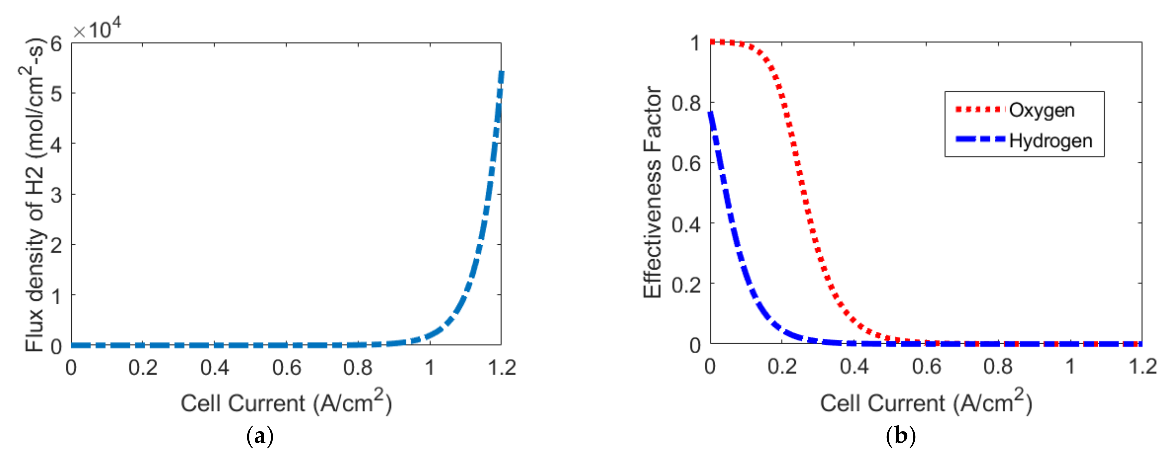
| Limiting current density | 1.4 A.cm−2 |
| Molar fraction of H2 in the anode () | 0.5 |
| Molar fraction of O2 at the inlet () | 0.21 |
| Molar fraction of O2 at the outlet () | 0.095 |
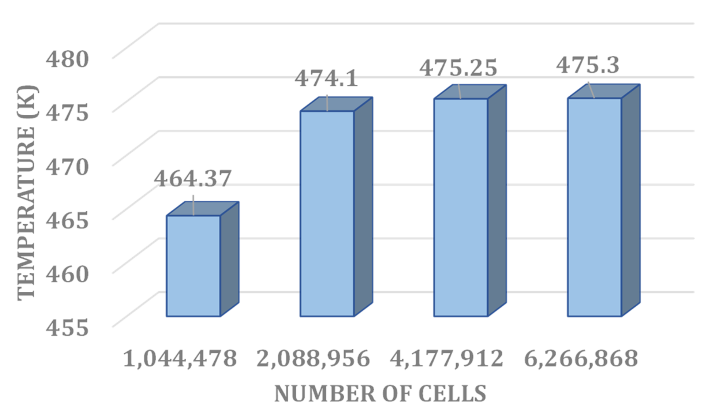
| Number of cells () | 90 |
| Operating pressure (anode and cathode side) (P) | 1 atm |
| Operating temperature (T) | 353.15 K |
| Reference temperature () | 298.15 K |
| Anodic/cathodic symmetry charge transfer coefficient () | 0.5 |
| Engine Mode | Engine Rotation Speed (min−1) | Torque (N.m) | Temperature (K), Present Study | Temperature (K), Fernández-Yañez et al. [28] | Pressure Drop (Pa), Present Study | Pressure Drop (Pa), Fernández-Yañez et al. [28] |
|---|---|---|---|---|---|---|
| A | 1000 | 10 | 388 | 387 | 110 | 119 |
| I | 2400 | 120 | 663 | 691 | 876 | 890 |
| G | 1000 | 120 | 583 | 658 | 211 | 253 |
| D | 1000 | 60 | 475 | 484 | 156 | 159 |
Publisher’s Note: MDPI stays neutral with regard to jurisdictional claims in published maps and institutional affiliations. |
© 2022 by the authors. Licensee MDPI, Basel, Switzerland. This article is an open access article distributed under the terms and conditions of the Creative Commons Attribution (CC BY) license (https://creativecommons.org/licenses/by/4.0/).
Share and Cite
Pourrahmani, H.; Shakeri, H.; Van herle, J. Thermoelectric Generator as the Waste Heat Recovery Unit of Proton Exchange Membrane Fuel Cell: A Numerical Study. Energies 2022, 15, 3018. https://doi.org/10.3390/en15093018
Pourrahmani H, Shakeri H, Van herle J. Thermoelectric Generator as the Waste Heat Recovery Unit of Proton Exchange Membrane Fuel Cell: A Numerical Study. Energies. 2022; 15(9):3018. https://doi.org/10.3390/en15093018
Chicago/Turabian StylePourrahmani, Hossein, Hamed Shakeri, and Jan Van herle. 2022. "Thermoelectric Generator as the Waste Heat Recovery Unit of Proton Exchange Membrane Fuel Cell: A Numerical Study" Energies 15, no. 9: 3018. https://doi.org/10.3390/en15093018
APA StylePourrahmani, H., Shakeri, H., & Van herle, J. (2022). Thermoelectric Generator as the Waste Heat Recovery Unit of Proton Exchange Membrane Fuel Cell: A Numerical Study. Energies, 15(9), 3018. https://doi.org/10.3390/en15093018