Thermal Design of a Biohydrogen Production System Driven by Integrated Gasification Combined Cycle Waste Heat Using Dynamic Simulation

Abstract

Utilizing biological processes for hydrogen production via gasification is a promising alternative method to coal gasification. The present study proposes a dynamic simulation model that uses a one-dimensional heat-transfer analysis method to simulate a biohydrogen production system. The proposed model is based on an existing experimental design setup. It is used to simulate a biohydrogen production system driven by the waste heat from an integrated gasification combined cycle (IGCC) power plant equipped with carbon capture and storage technologies. The data from the simulated results are compared with the experimental measurement data to validate the developed model’s reliability. The results show good agreement between the experimental data and the developed model. The relative root-mean-square error for the heat storage, feed-mixing, and bioreactor tanks is 1.26%, 3.59%, and 1.78%, respectively. After the developed model’s reliability is confirmed, it is used to simulate and optimize the biohydrogen production system inside the IGCC power plant. The bioreactor tank’s time constant can be improved when reducing the operating volume of the feed-mixing tank by the scale factors of 0.75 and 0.50, leading to a 15.76% and 31.54% faster time constant, respectively, when compared with the existing design.

1. Introduction

Coal gasification is a flexible technology that utilizes syngas to generate energy and produce chemical products [1]. An integrated gasification combined cycle (IGCC) power plant uses this technology to efficiently produce electricity while minimizing the environmental impact [2]. The use of coal in this fuel power-generation process is concerning, as it is closely associated with carbon dioxide (${\mathrm{CO}}_2$) emissions that negatively impact the environment if left uncontrolled. The reduction of ${\mathrm{CO}}_2$ emissions is one of the most important factors to be considered when it comes to future power generation as an active means to combat climate change. Since fossil fuels will likely remain a primary energy source in the future, there is a strong need to develop power-generation technologies with a reduced fossil ${\mathrm{CO}}_2$ footprint [3]. Coal as a power-generation fuel can only be considered sustainable if ${\mathrm{CO}}_2$ is captured and stored in suitable geologic formations for a long time [4].

The development of carbon capture and storage (CCS) technologies is expected to play a crucial role in reducing greenhouse gas emissions. The CCS technologies group uses various energy-conversion systems and other energy-intensive industrial applications (e.g., cement production and petrochemistry) to reduce fossil ${\mathrm{CO}}_2$ emissions [5]. The IGCC generates electricity using solid feedstock (i.e., coal, lignite, biomass, and solid waste) that is partially oxidized with oxygen by air separation unit steam to produce syngas, a mixture of carbon monoxide (CO) and hydrogen. Besides generating electricity, the IGCC process is capable of coproducing hydrogen and steam [6]. In an IGCC power plant integrated with CCS technologies, the ash and hydrogen sulfide are removed in the gasification process in a catalytic water–gas shift (WGS) reaction to treat the syngas [4]. The WGS chemical reaction process allows the syngas thermal energy to be concentrated in the form of hydrogen and a carbon species in the state of ${\mathrm{CO}}_2$ based on the following reaction equation [4]:

$$\mathrm{C}\mathrm{O}+{\mathrm{H}}_2\mathrm{O}\leftrightarrow \mathrm{C}{\mathrm{O}}_2+{\mathrm{H}}_2$$

(1)

Hydrogen coproduction in IGCC power plants is a common process and has been extensively discussed in previous studies [2,5,6,7,8,9]. This feature has enhanced the robustness of IGCC power plant applications since these plants must improve in both operation and availability to succeed as alternative power-generation facilities that supersede conventional coal-fired power plants. Nevertheless, integrating CCS technologies into the current IGCC power plant system has been estimated to increase 22.5% in investment cost when a 90% CCS capture rate is implemented [6]. Fortunately, the coproduction of pure hydrogen helps mitigate the drawbacks of implementing CCS technologies since pure hydrogen has a high added value and can be used for energy and industrial uses [4,6].

In recent years, hydrogen has become an essential renewable secondary energy carrier for various applications and is expected to play a crucial role in the future of energy systems. Generally, hydrogen is used for multiple purposes, such as crude oil desulfurization or electronic device production [10]. Nevertheless, it is predominantly produced from fossil fuels; hydrogen gas is primarily supplied by natural gas steam reforming and water electrolysis processes [11]. Nonetheless, these methods are intensive and require high energy to provide hydrogen as an energy source. Biological methods offer a promising alternative solution for the future production of hydrogen. A biological hydrogen production method is more advantageous in operating conditions than the conventional chemical methods [12,13].

Biohydrogen has a clean energy carrier property since it has a high energy yield in the combustion of hydrogen fuel, where the major byproduct is only water (${\mathrm{H}}_2\mathrm{O}$) molecule emission in the environment [14,15]. Additionally, hydrogen fuel’s renewable characteristics produced via bioproduction can be developed from various biological routes (i.e., utilizing biological waste as the potential source of biohydrogen provides a new avenue for the utilization of renewable sources) [16,17]. The biohydrogen production processes can be categorized into several groups: photobiological fermentation, dark fermentation, anaerobic fermentation, and thermochemical and enzymatic processes [10,14,18,19]. Biohydrogen can be produced through various methods, e.g., anoxic photosynthesis, fermentation, oxygenic photosynthesis, and cyanobacterial hydrogen biosynthesis through a nitrogenase enzyme complex [19].

Although dark fermentation methods are well-established and offer integrative prospects, they are still uncommon in the industry [20]. Past studies have reported that dark fermentation has the advantage of a high production rate; nevertheless, it offers a lower yield compared with other methods [21,22,23]. For the past decade, the production rate of the dark fermentation method has been steadily increasing because of the development of stable compartments of mixed strains; furthermore, the stability of these strains has been enhanced by advanced technologies [24,25,26,27,28,29]. Based on previous studies, a dark fermentation approach has been developed whereby a hyperthermophile-type bacterium called Thermococcus onnurineus NA1 can be used as a biocatalyst in a WGS reaction to produce hydrogen; in this approach, the bacterium feeds on a CO-rich gas [24,25]. The NA1 strain is genetically engineered and possesses high activity for the bioconversions of industrial waste gases created from the byproducts of steel production; these bioconversions produce hydrogen via a WGS chemical reaction process [25,30]. The benefits of using the byproduct gases from steel mill processes for hydrogen production are a high yield and reduced cost [25]. A separate study reported that Linz–Donawitz gas and blast furnace gas could also be used for hydrogen production using Thermococcus onnurineus NA1 [30,31]. Besides the waste gas from steel mills, the syngas from the coal gasification process could be used as the primary source of CO in a WGS reaction for hydrogen production [32].

In the bioconversion operating conditions for hydrogen production using Thermococcus onnurineus NA1, temperature is an essential factor for activation of the bacterium to produce hydrogen [25]. The optimal temperature for the bacterium to be activated in the WGS reaction is 80 °C [25,30,33]. Note that pressure is not as significant as CO solubility [33]. The hydrogen productivity can be increased when the CO solubility is increased by applying more pressure if the toxicity of the CO is endurable for the bacterium [33]. Additionally, the highest and most productive hydrogen production is achieved when Thermococcus onnurineus NA1 is pressurized up to 4 bar [33].

This study focuses on utilizing the syngas and waste heat from an IGCC power plant with CCS to produce hydrogen. In such a power plant, the syngas is made from the coal gasification process, and it is primarily comprised of hydrogen, CO, CO₂, nitrogen, and methane. Thus, the syngas is used as the source of CO in the WGS reaction process. As for the waste heat from the IGCC power plant, the heat recovered from the exhaust gas of the gas turbine system through the heat recovery steam generator (HRSG) will act as the primary heat source for the biohydrogen production system. The exhaust gas from the gas turbine system will be transferred to HRSG to extract their heat and transfer the heat to steam via a heat exchanger. The heated steam will be sent to a steam boiler, where its pressure is lowered and used to supply heat to the biohydrogen production system. Furthermore, the flue gas from the HRSG can also be used as the waste heat source for the biohydrogen production system [34].

The motivation for this study comes from the fact that there is no systematic implementation of the hydrogen production process produced biologically from the bacterium Thermococcus onnurineus NA1 driven by the waste heat from IGCC power plants. To the best of the authors’ knowledge, this is the first application of biohydrogen production driven by IGCC power plant waste heat from HRGS. Hence, mathematical modeling of the system is crucial in evaluating and optimizing it for future studies. Thus, a dynamic model was developed to simulate the system’s thermal behavior based on the given boundary conditions.

A dynamic mathematical model that can carry out the simulation or thermal design optimization of a biohydrogen production system is necessary when various parameters are considered in the system’s design process. For instance, the system’s thermal behavior may differ if operating in a cold versus hot environment. In a cold environment, more heat may be needed to maintain the desired operating conditions for hydrogen production. However, the amount of heat supplied must be appropriate so that the system can operate properly and ensure the hydrogen production process is not interrupted due to overheating. Thus, the developed model can be utilized to determine the correct amount of heat.

Another advantage of having a model that can simulate the biohydrogen production system is that it can be used to estimate how much waste heat is required for the system to operate correctly. In the IGCC power plant, the HRSG also needs to supply heated steam to the steam turbine to generate electricity. The steam supply to the steam turbine might be interrupted when the biohydrogen production system is implemented in the IGCC power plant as an additional auxiliary system. Therefore, it is crucial to determine the amount of continuous waste heat required by the system that should be pre-allocated to ensure that the IGCC power plant operation process will not be interrupted.

As mentioned previously, the coproduction of hydrogen with the IGCC power plant could help mitigate the economic drawbacks of implementing CCS technologies in the plant. Nevertheless, the size of the implemented biohydrogen production system as an auxiliary component of the IGCC power plant will impact the investment and operational cost for the whole plant. Therefore, the simulation model can optimize a detailed unit sizing and thermal design of the system’s components, such as the bioreactor tank and heat exchanger, to reduce these costs. Additionally, the optimization process through the simulation model can help find the best configuration for the biohydrogen production system.

This study focuses on mathematical dynamic model development based on a lab-scale biohydrogen production system utilizing the heat-transfer lumped analysis method. The chosen method is implemented in the model development due to assessment simplicity. Additionally, this method is used for various configurations or cases as long as the requirements to use it are fulfilled. Thus, one of this study’s main goals is to create a model that can be applied to various configurations, including lab-scale models and actual plants.

To ensure that the developed model can be applied to various configurations, this study focuses on the heat transfer of the feed-mixing and bioreactor tanks in the biohydrogen production system. The feed-mixing tank’s role is to be the cultivation containment tank for the bacterium’s active hydrogen production, where it is fed nutrients in the cultivation process. By contrast, the bioreactor tank is where the WGS process and the produced hydrogen collection occur. Both tanks are necessary for any biohydrogen production system. Hence, the current model development sets the feed-mixing and bioreactor tanks as core components in various configurations, including lab-scale models and actual plants.

The model’s reliability is evaluated based on the experimental result of the lab-scale biohydrogen production system. After the reliability of the code is confirmed, the system’s configuration is changed to the design of the IGCC power plant’s biohydrogen production system. The only changes that are made are to the system’s configuration; the approach to evaluate the thermal analysis in the developed mathematical model remains the same. The present study also conducts a thermal design analysis and an optimization investigation using a dynamic simulation of a biohydrogen production system driven by IGCC waste heat.

The motivation of this study is to propose a dynamic mathematical model that can provide a heat-transfer analysis of the biohydrogen production system driven by the IGCC waste heat to carry out evaluation and optimization tasks. In order to achieve this purpose, a biohydrogen production system that utilizes the unique properties of Thermococcus onnurineus NA1 in producing hydrogen through the dark fermentation method is selected in the present study. The selected biohydrogen production system is integrated into the IGCC power plant operation process in order to establish a hydrogen coproduction process in the power plant. The IGCC waste heat drives the established hydrogen coproduction process, which will help in mitigating the drawbacks of implementing CCS technologies in the IGCC power plant operation process.

The present study provides a dynamic mathematical model representing the heat and mass transfer analysis of the biohydrogen production system’s component driven by the IGCC waste heat. This study also discusses the details of the chosen heat-transfer analysis method and the heat and mass transfer equations in developing the proposed model. Finally, the proposed model is validated based on the lab-scale biohydrogen production system experiment. The current work also conducts a thermal design analysis and an optimization investigation based on the developed model as mentioned previously.

2. Mathematical Simulation Modeling

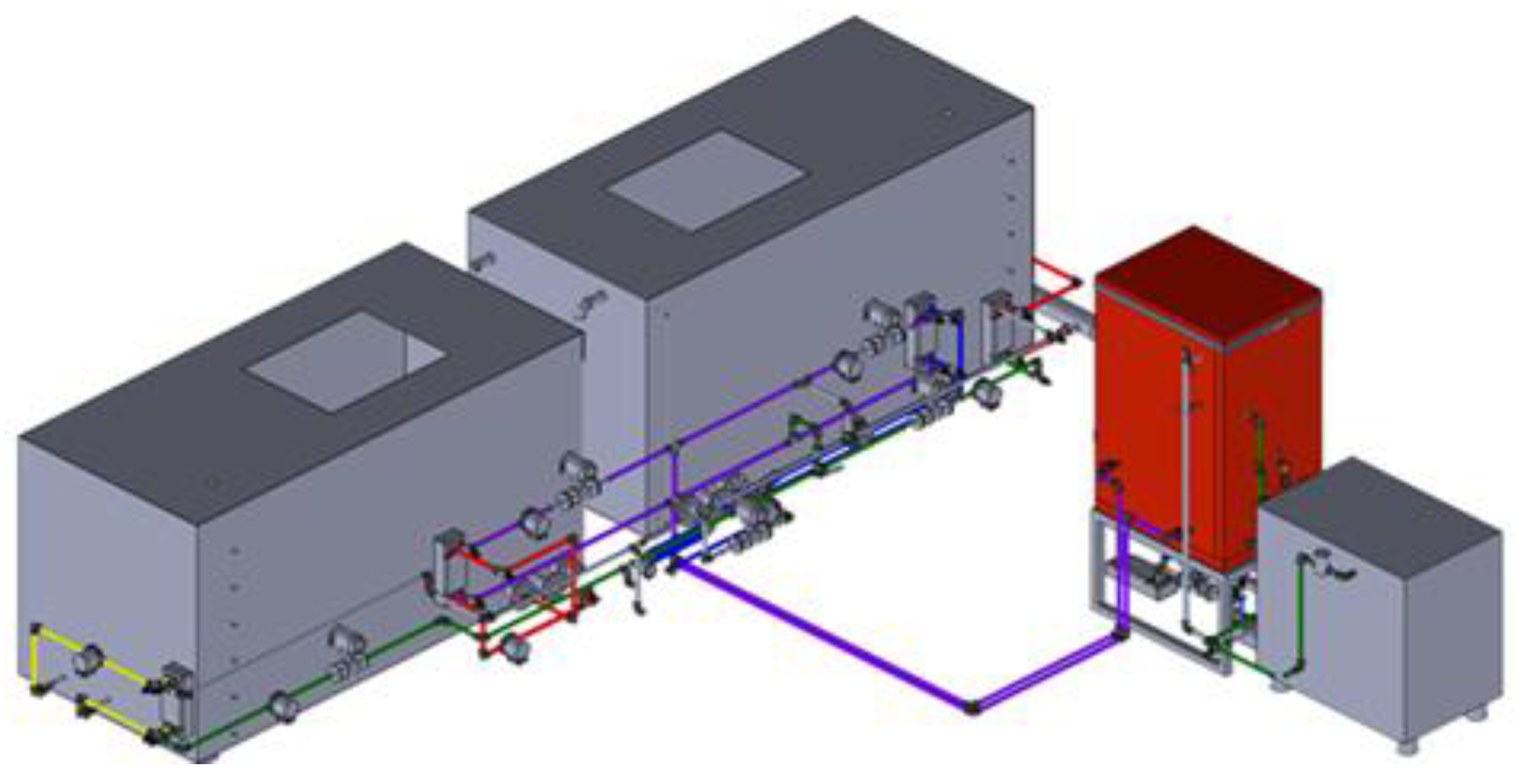
The present study simulates two models of a biohydrogen production system, i.e., the validation model and the bio-IGCC model. The validation model is based on the experimental design of a lab-scale biohydrogen production system that serves as the industrial application pilot study. Figure 1 illustrates the three-dimensional, computer-aided design drawing of the experimental setup of the lab-scale biohydrogen production system. 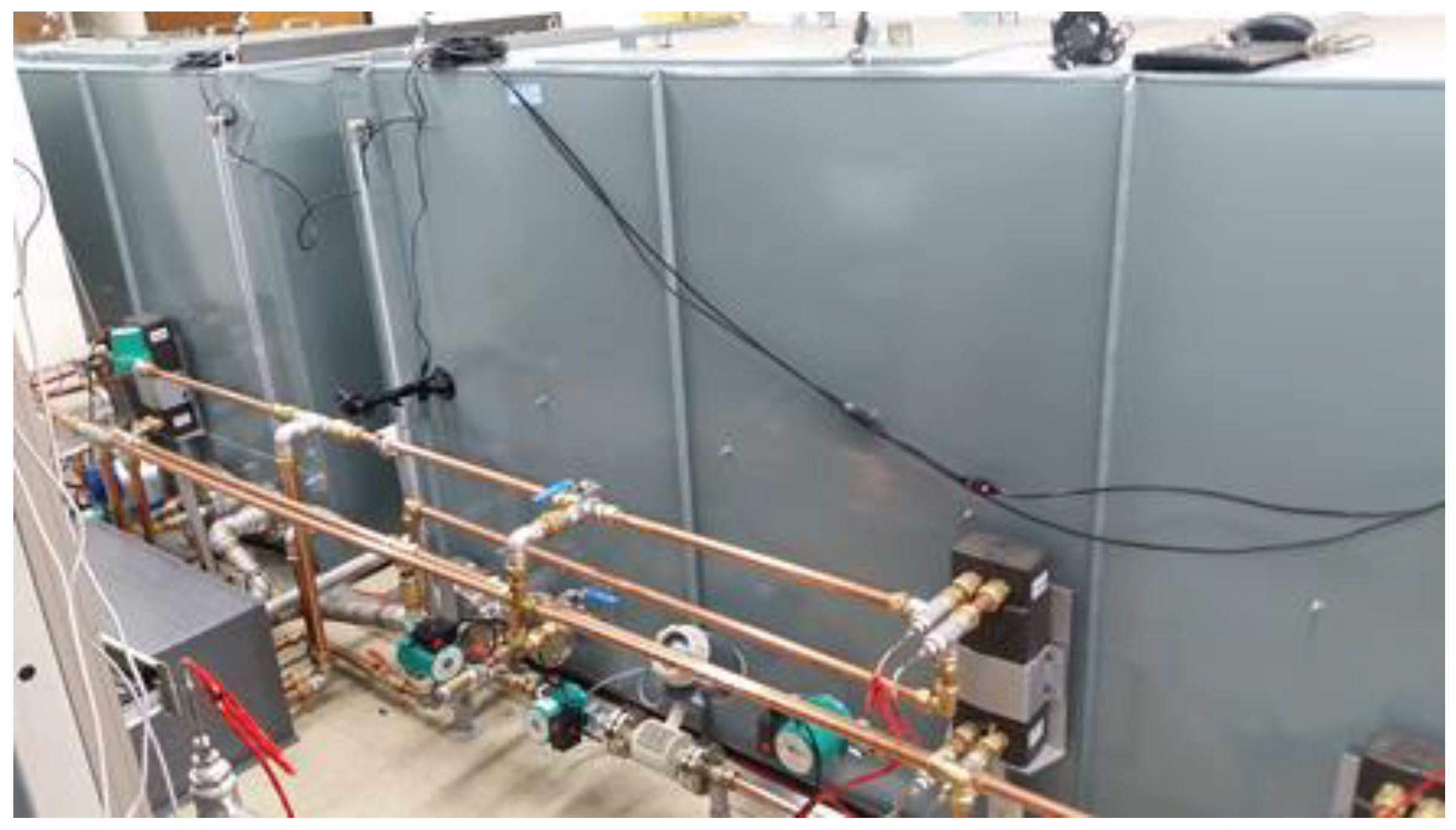Figure 2 shows the picture of the experiment setup facility.

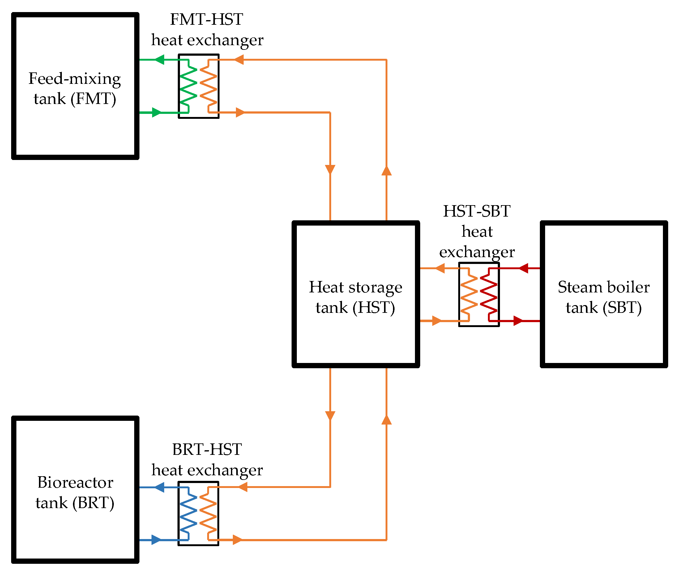
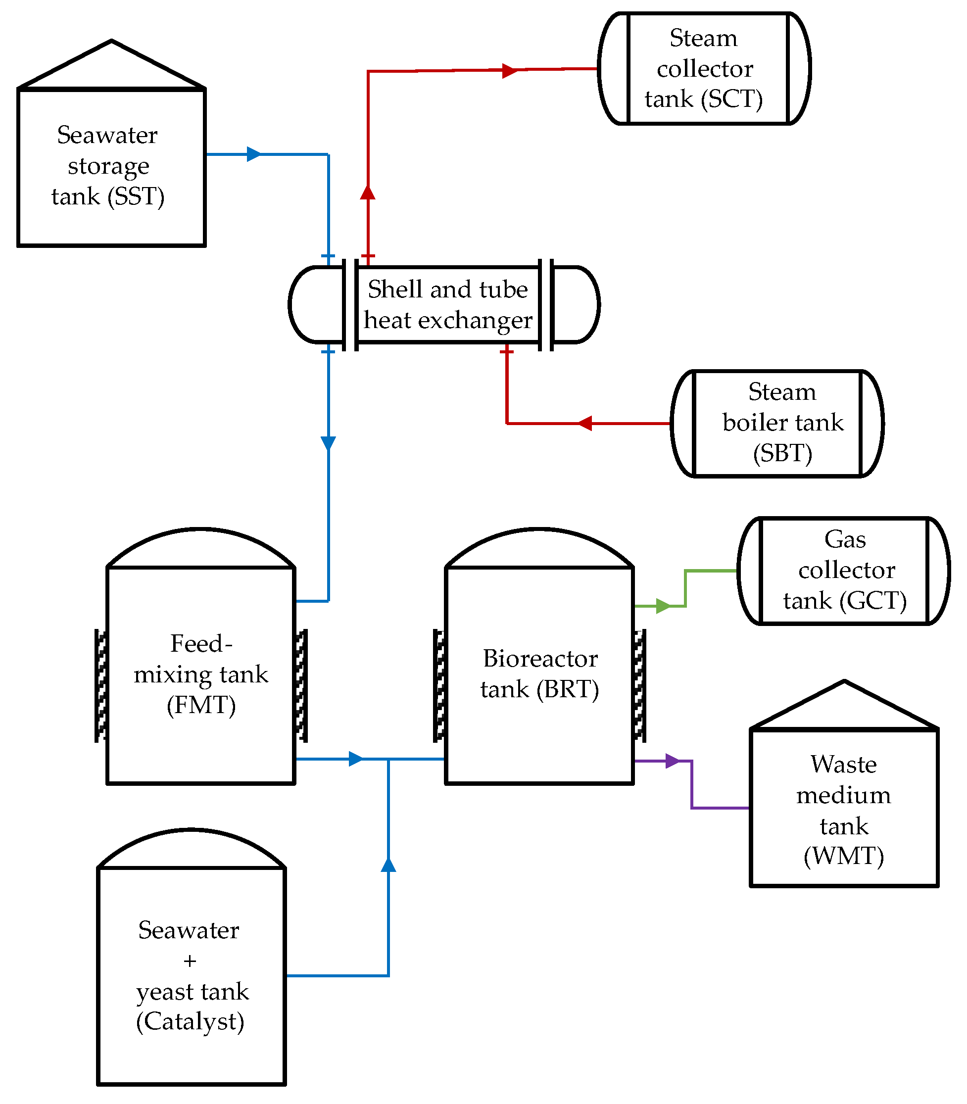
The validation model is used to verify the heat-transfer analysis method utilized in the mathematical modeling of the simulation. The bio-IGCC model is based on a biohydrogen production–IGCC power plant system design (this paper’s case study). Figure 3 and Figure 4 illustrate the graphical diagrams representing the configuration for both systems. Although the designs are slightly different, steam is still the primary heat source for both systems.

In this study’s lab-scale biohydrogen production system experiment, it was determined that the amount of time for the bioconversion in the hydrogen production using Thermococcus onnurineus NA1 is approximately 6 h. Thus, the amount of time the fluid was stored inside the bioreactor tank for the bio-IGCC model was also 6 h to simulate the bioconversion process.

The critical components of the biohydrogen production system that this study investigates are the heat-exchanger, feed-mixing, and bioreactor tanks. The role of the bioreactor tank is the production and collection of hydrogen through the WGS chemical reaction. The feed-mixing tank is where Thermococcus onnurineus NA1 is cultured before sending it to the bioreactor. The working fluid used in the model, i.e., the cultured Thermococcus onnurineus NA1 mixed with water, can be treated like seawater, as it has a salinity of 3.5%. The heat-exchanger tank is used to exchange heat with the primary heat source to heat the bioreactor and feed-mixing tanks to the desired operating condition.

The main focus in the model development is the thermal aspect of the current design of biohydrogen production. Thus, the heat and mass transfer analysis approach is used to simulate the system’s behavior on the basis of the determined boundary conditions. A validation process is conducted to ascertain the validity of the heat-transfer analysis approaches used to develop the model by comparing the results of the developed model with experimental results. The following assumptions are made to simplify the system to be simulated and modeled:

• The fluid inside the tank is perfectly mixed due to the tank’s significant amount of operating volume;
• The heat from the biological WGS is ignored, as the reaction’s heat is relatively nominal compared with the heat generated by the whole system;
• The inlet and outlet of each system element are steady state.

For the dynamic simulation modeling of the biohydrogen production system, this study uses a lump capacitance approach for the system modeling. To use the lump capacitance method, the Biot number ($Bi$) of the tanks in the studied system must be less than 0.1. Thus, the validation of the tanks in the modeling of each system using the lump capacitance method is evaluated. The $Bi$ equation is expressed as follows [35]:

$$Bi=\frac{h_{\mathrm{conv}}{L}_{\mathrm{c}}}{k_{\mathrm{solid}}}$$

(2)

Here, $h_{\mathrm{conv}}$ is the convective heat-transfer coefficient, $L_{\mathrm{c}}$ is the characteristic length, and $k_{\mathrm{solid}}$ is the solid thermal conductivity.

2.1. Validation Model Biohydrogen Production System

The validation model of the biohydrogen production system consisted of a bioreactor tank, feed-mixing tank, plate heat exchange, steam boiler, and heat storage tank. The steam boiler was the primary heat source to heat the bioreactor and the feed-mixing tank to the desired operating condition. The heat storage tank acted as the intermediate medium to recover the heat from the steam boiler via a plate heat exchanger. Furthermore, the steam boiler was treated as the industrial waste heat source used for the actual application. Steam was used to transfer the industrial process waste heat to the biohydrogen production system in the actual application.

A Danfoss brazed plate heat exchanger (model XB-06H-1-26-H) was used in the experimental setup. In the developed model, the effectiveness number of transfer units method was applied to determine the temperature outlets of the cold and hot sides of the heat exchanger [35]. 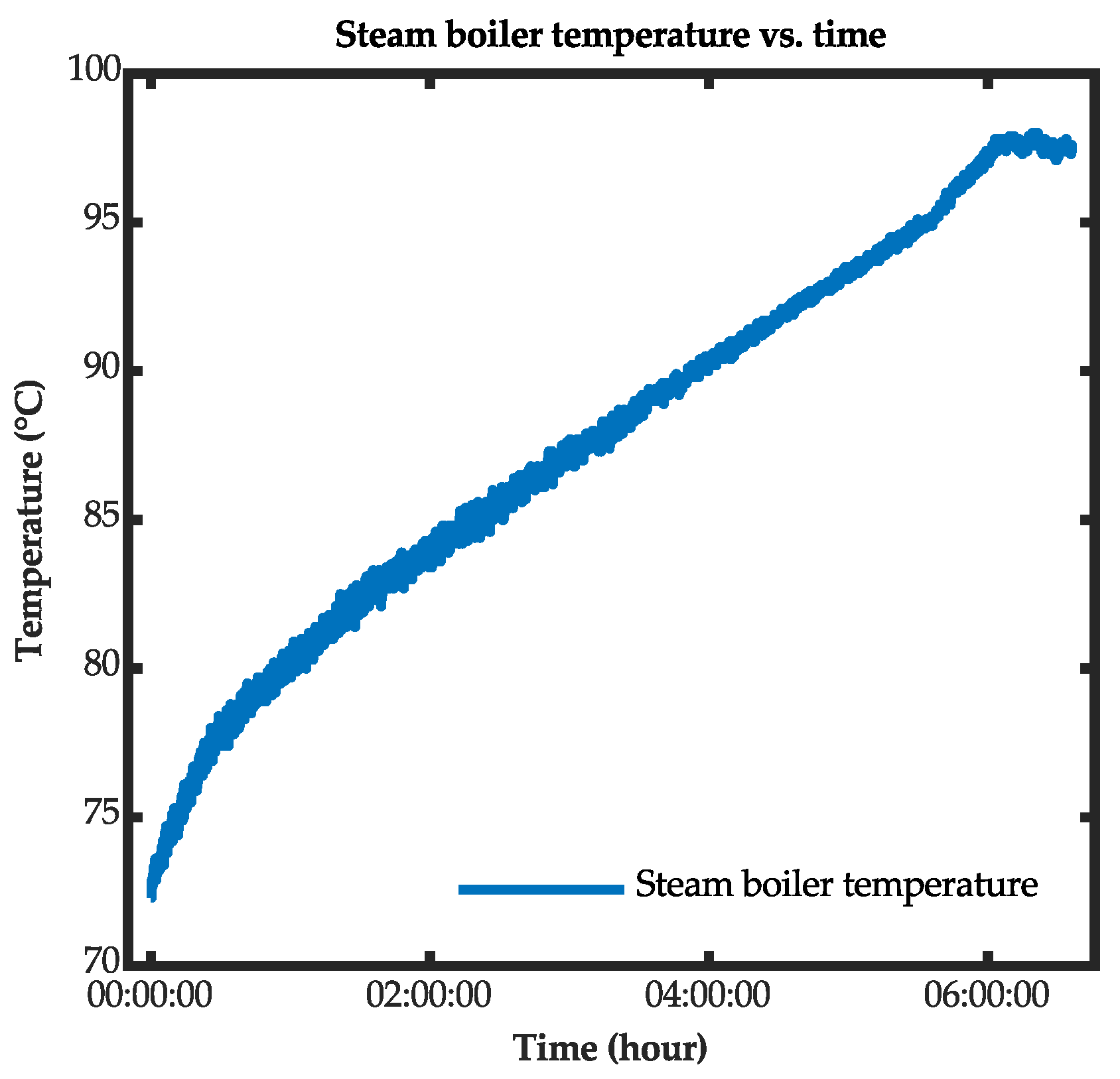Danfoss commercial software (Danfoss Hexact, version: 5.5.24, Creator: Danfoss A/S, Location: Nordborg, Denmark) was used to determine the heat-transfer coefficient for the hot and cold sides of the heat exchanger and the overall heat-transfer equation [36]. The temperature profile for the outlet of the steam boiler is illustrated in Figure 5 (the hot side of the heat exchanger). The cold side was filled with the fluid from the heat storage tank. The flow of the heat-transfer process from the steam boiler to the bioreactor and feed-mixing tanks can be described as follows:

• The steam exchanged heat with the water from the heat storage tank;
• The heated water from the heat storage tank exchanged heat with the fluid from the feed-mixing and bioreactor tanks.

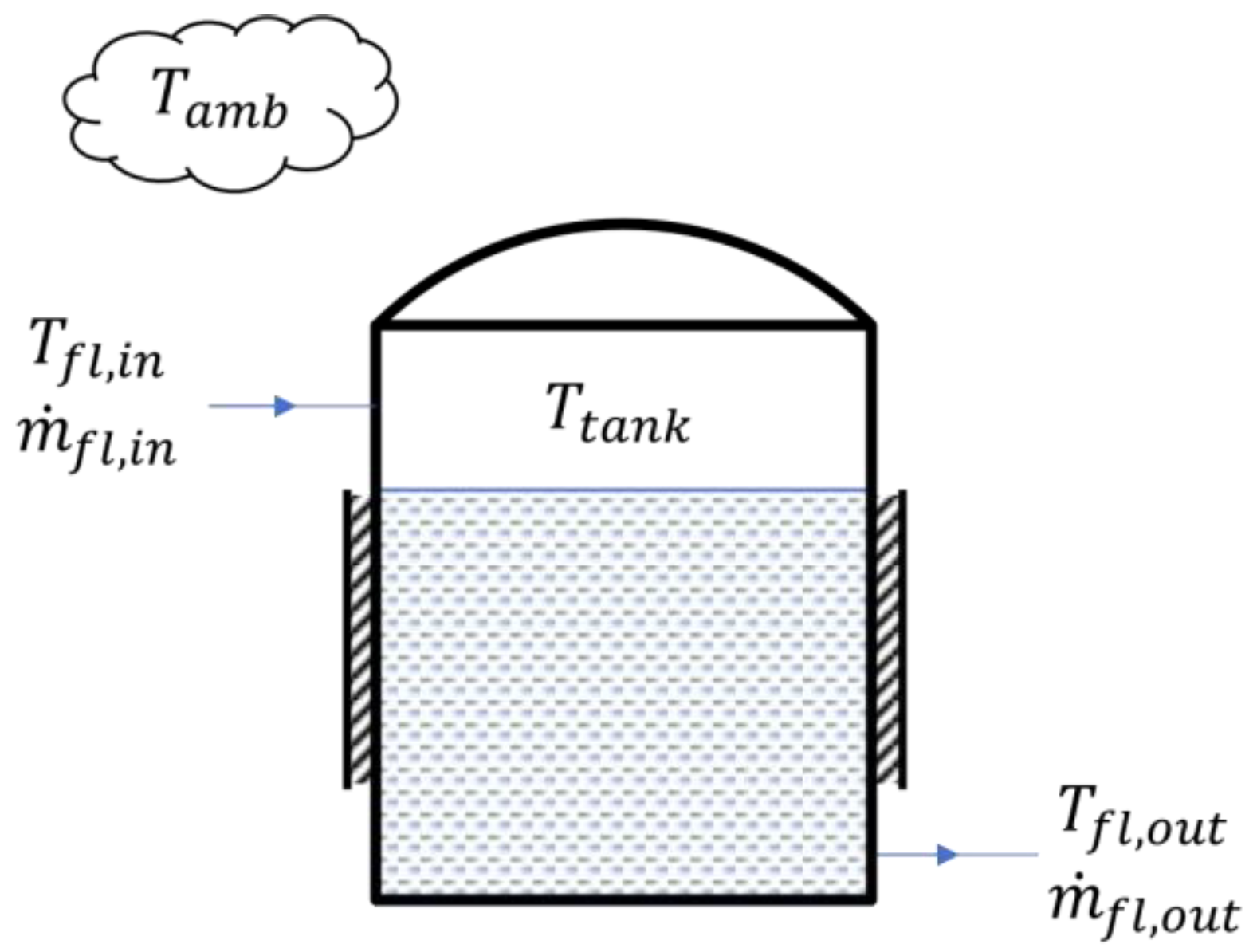
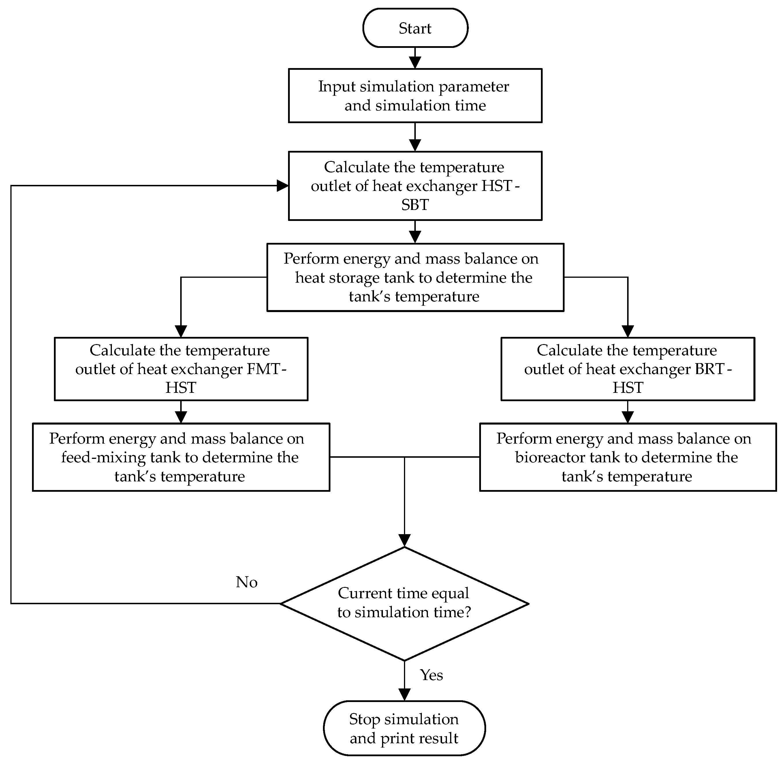
The analysis of the heat and mass transfer interaction for each of the tanks in the lab-scale biohydrogen production system is illustrated in Figure 6. The generalized dynamic equations that determined the tank’s temperature and volume were analyzed and developed for the simulation based on the analysis conducted. These calculations are expressed in Equations (3) and (4).

$$\frac{d{T}_{\mathrm{tank}}}{dt}=\frac{1}{V_{\mathrm{tank},\mathrm{fl}}{\rho }_{\mathrm{fl}}{c}_{\mathrm{p},\mathrm{fl}}}\left[{\dot{m}}_{\mathrm{fl},\mathrm{in}}{c}_{\mathrm{p},\mathrm{fl}}\left(T_{\mathrm{fl},\mathrm{in}}-T_{\tan \mathrm{k}}\right)-{\dot{m}}_{\mathrm{fl},\mathrm{out}}{c}_{\mathrm{p},\mathrm{fl}}\left(T_{\mathrm{fl},\mathrm{out}}-T_{\tan \mathrm{k}}\right)+U_{\mathrm{amb},1}\left(T_{\tan \mathrm{k}}-T_{\mathrm{amb}}\right)\right]$$

(3)

$$\frac{d{V}_{\mathrm{tank}}}{dt}=\frac{{\dot{m}}_{\mathrm{fl},\mathrm{in}}c-{\dot{m}}_{\mathrm{fl},\mathrm{out}}}{{\rho }_{\mathrm{fl}}}$$

(4)

Here, $T_{\mathrm{tank}}$ is the temperature of the fluid inside the tank; $V_{\mathrm{tank},\mathrm{fl}}$ is the volume of the fluid inside the tank; $c_{\mathrm{p},\mathrm{fl}}$ is the specific heat capacity of the fluid inside the tank; ${\dot{m}}_{\mathrm{fl},\mathrm{in}}$ and ${\dot{m}}_{\mathrm{fl},\mathrm{out}}$ are the mass flow rates at the inlet and outlet of the tank, respectively; $T_{\mathrm{fl},\mathrm{in}}$ and $T_{\mathrm{fl},\mathrm{out}}$ are the temperatures at the inlet and outlet of the tank, respectively; $U_{\mathrm{amb},1}$ is the overall heat-transfer coefficient between the fluid inside the tank and the ambient air; and $T_{\mathrm{amb}}$ is the ambient temperature.

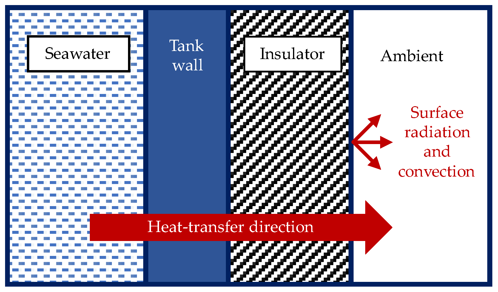
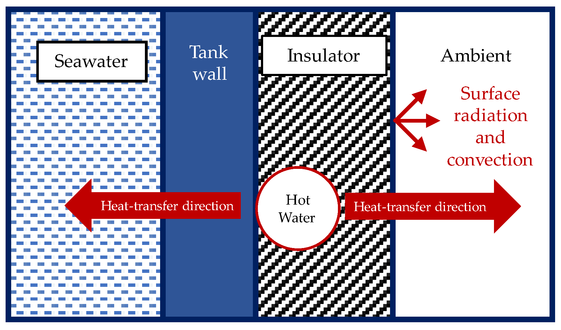
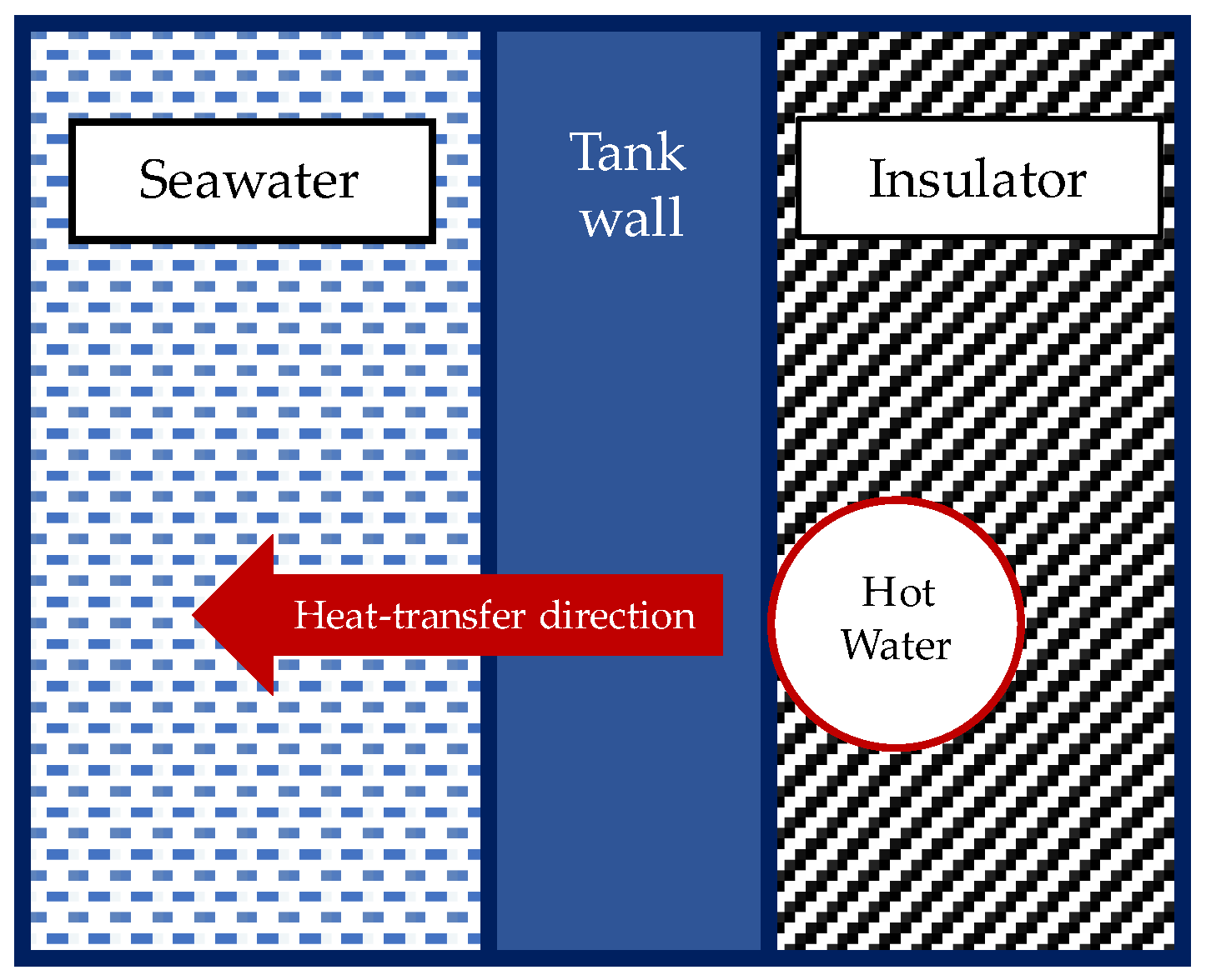
Figure 7 shows the heat-transfer direction from the fluid inside the tank to the ambient air. Based on the interaction shown in Figure 7, the overall heat-transfer coefficient between the fluid inside the tank and the ambient air could be determined and expressed by Equation (5) and obtained through one-dimensional thermal resistance circuit analysis [35]. The tank walls and insulators were treated as flat plates for the geometrical properties. The Nusselt number equation used to determine the convective heat-transfer coefficient in the Equation (6) is shown in Equation (7) [35]. The correlation expressed in the Equation (7) can be applied over the entire range of the Rayleigh number and applicable to a vertical flat geometry. In terms of geometry, the tank’s wall for the validation model will be treated as a flat plate for the thermal resistance circuit analysis based on the design of the tanks, as illustrated in Figure 1.

$$U_{\mathrm{amb},1}=\frac{1}{h_{\mathrm{conv},\mathrm{fl}}{A}_{\mathrm{wall}}}+\frac{t_{\mathrm{wall}}}{k_{\mathrm{wall}}{A}_{\mathrm{wall}}}+\frac{t_{\mathrm{ins}}}{k_{\mathrm{ins}}{A}_{\mathrm{ins}}}+\frac{1}{\frac{1}{h_{\mathrm{conv},\mathrm{amb}}{A}_{\mathrm{ins}}}+\frac{1}{h_{\mathrm{rad},\mathrm{amb}}{A}_{ins}}}$$

(5)

$$h_{\mathrm{conv}}=\frac{N{u}_L{k}_{\mathrm{fl}}}{L_{\mathrm{c}}}$$

(6)

$$N{u}_{\mathrm{L}}={\left[0.825+\frac{0.387{\mathrm{Ra}}_{\mathrm{L}}{}^{1/6}}{{\left(1+{\left(0.492/{\mathrm{Pr}}_{\mathrm{fl}}\right)}^{9/16}\right)}^{8/27}}\right]}^2$$

(7)

$$h_{\mathrm{rad},\mathrm{amb}}={\epsilon }_{\mathrm{ins}}\sigma \left(T_{\mathrm{s}}-T_{\mathrm{amb}}\right)\left(T_{\mathrm{s}}{}^2-T_{\mathrm{amb}}{}^2\right)$$

(8)

In these equations, $h_{\mathrm{conv},\mathrm{fl}}$ is the convective heat-transfer coefficient of the fluid in the tank, $h_{\mathrm{conv},\mathrm{amb}}$ is the convective heat-transfer coefficient at the ambient air and insulator interface, $A_{\mathrm{wall}}$ is the heat-exchange area of the tank wall, $A_{\mathrm{ins}}$ is the heat-exchange area of the insulator, $t_{\mathrm{wall}}$ is the thickness of the tank wall, $t_{\mathrm{ins}}$ is the thickness of the insulator, $k_{\mathrm{wall}}$ is the thermal conductivity of the tank wall, $k_{\mathrm{ins}}$ is the insulator thermal conductivity, ${\mathrm{Ra}}_{\mathrm{L}}$ is the Rayleigh number, ${\mathrm{Pr}}_{\mathrm{fl}}$ is the Prandtl number of the fluid inside the tank, $h_{\mathrm{rad},\mathrm{amb}}$ is the radiative heat-transfer coefficient at ambient, ${\epsilon }_{\mathrm{ins}}$ is the emissivity of the insulator, $\sigma$ is the Stefan–Boltzmann constant, and $T_{\mathrm{s}}$ is the surface temperature of the insulator.

2.2. Integrated Gasification Combined Cycle Biohydrogen Production System Model

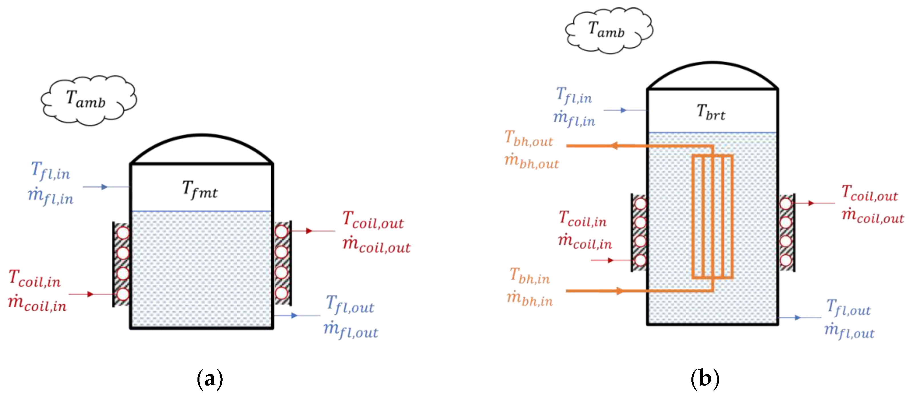
For the IGCC power plant biohydrogen production system, the low steam pressure from the IGCC power-generation process was the waste heat source from the IGCC power plant that was recovered through a shell and tube heat exchanger. The fluid inside the feed-mixing tank was heated with the recovered heat. The temperature outlet of the heat exchanger was set at 90 °C. Figure 8 illustrates the simplified structures of the feed-mixing and bioreactor tanks as well as their heat interaction. As is shown in the figure, both of the tanks were cylindrical structures equipped with an external coil heater and insulator. Nevertheless, the bioreactor tank had an additional vertical bundle heater inside the reactor. The purpose of adding the heaters was to heat and maintain the fluid temperature inside the tanks at optimal conditions in large quantities.

The developed dynamic equations for determining the temperatures of the feed-mixing tank and the bioreactor tank in the bio-IGCC model are expressed in Equations (9) and (10), respectively.

$$\frac{d{T}_{\mathrm{fmt}}}{dt}=\frac{1}{V_{\mathrm{fmt}}{\rho }_{\mathrm{fl}}{c}_{\mathrm{p},\mathrm{fl}}}\left[\left({\dot{m}}_{\mathrm{fl},\mathrm{in}}{c}_{\mathrm{p},\mathrm{fl}}\left(T_{\mathrm{fl},\mathrm{in}}-T_{\mathrm{fmt}}\right)+U_{\mathrm{coil}}\left({\mathrm{T}}_{\mathrm{coil}}-T_{\mathrm{fmt}}\right)\right)-\left({\dot{m}}_{\mathrm{fl},\mathrm{out}}{c}_{\mathrm{p},\mathrm{fl}}\left(T_{\mathrm{fl},\mathrm{out}}-T_{\mathrm{fmt}}\right)+U_{\mathrm{amb}}\left(T_{\mathrm{fmt}}-T_{\mathrm{amb}}\right)\right)\right]$$

(9)

$$\frac{d{T}_{\mathrm{brt}}}{dt}=\frac{1}{V_{\mathrm{brt}}{\rho }_{\mathrm{fl}}{c}_{\mathrm{p},\mathrm{fl}}}\left[\begin{array}{l}\left({\dot{m}}_{\mathrm{fl},\mathrm{in}}{c}_{\mathrm{p},\mathrm{fl}}\left(T_{\mathrm{fl},\mathrm{in}}-T_{\mathrm{brt}}\right)+U_{\mathrm{coil}}\left(T_{\mathrm{coil}}-T_{\mathrm{brt}}\right)+U_{\mathrm{bh}}\left(T_{\mathrm{bh}}-T_{\mathrm{brt}}\right)\right)\\ -\left({\dot{m}}_{\mathrm{fl},\mathrm{out}}{c}_{\mathrm{p},\mathrm{fl}}\left(T_{\mathrm{fl},\mathrm{out}}-T_{\mathrm{brt}}\right)+U_{\mathrm{amb},2}\left(T_{\mathrm{brt}}-T_{\mathrm{amb}}\right)\right)\end{array}\right]$$

(10)

Here, $T_{\mathrm{fmt}}$ is the temperature of the fluid inside the feed-mixing tank; $T_{\mathrm{brt}}$ is the temperature of the fluid inside the bioreactor tank; $T_{\mathrm{coil}}$ is the fluid temperature inside the external heating coil; $T_{\mathrm{bh}}$ is the fluid temperature inside the vertical bundle; ${\rho }_{\mathrm{fl}}$ is the fluid density; $V_{\mathrm{fmt}}$ and $V_{\mathrm{brt}}$ are the fluid volumes inside the feed-mixing tank and bioreactor tank, respectively; and $U_{\mathrm{coil}}$, $U_{\mathrm{bh}}$, and $U_{\mathrm{amb},2}$ are the overall heat-transfer coefficient for the coil heater, the vertical bundle heater inside the bioreactor, and the heat loss to the ambient air, respectively.

The dynamic equation that determined the tank’s volume in the bio-IGCC model was similar to Equation (3). However, the fluid flow at the inlet of the bioreactor tank for the bio-IGCC model had two sources: the feed-mixing tank and heated seawater mixed with yeast that acted as a catalyst for Thermococcus onnurineus NA1. The role of the catalyst was to increase the reaction rate for hydrogen production, and it did not affect the heat-transfer process.

Figure 9 shows the directions of the heat transfer between the coil heater, the fluid in the tanks, and the ambient air. A one-dimensional thermal resistance circuit analysis was conducted at the wall of the tank covered by an insulator and a coil heater to determine the heat loss to its surroundings. For the heat transfer from the coil heater to the tank wall, it was assumed that 20% of the whole coil heater was in contact with the tanks, while the remaining area was in contact with the insulator. The fluid inside the coil heater was water at 90 °C.

Figure 10 illustrates the heat-transfer direction from the water inside the coil heater to the fluid inside the tank. The overall heat-transfer coefficient for the heat transfer from the coil heater to the fluid inside the tank is shown in Equation (11). Furthermore, the pre-calculation indicated that the flow inside the tank was laminar. In terms of geometry, the cylinder tank wall in this system model could be treated as a flat plate for the thermal resistance circuit analysis since the condition for the present case study was satisfied according to Equation (12) [35]. Because of this condition, the Nusselt number correlation expressed in Equation (7) could also be used for the inner side of the tank in the current system model. Equation (13) is the Nusselt number correlation used to determine the convective heat-transfer coefficient in the coil heater [37]. The thermal conduction resistance analysis along the walls of the feed-mixing tank and bioreactor tank covered by the insulator and the heater coil was expressed by Equations (16) and (18) [38].

$$U_{\mathrm{coil}}=\frac{1}{\frac{1}{h_{\mathrm{conv},\mathrm{fl}}{A}_{\mathrm{wall}}}+R_{\mathrm{cond},\mathrm{wall}}+R_{\mathrm{cond},\mathrm{coil}}\frac{1}{h_{\mathrm{conv},\mathrm{coil}}{A}_{\mathrm{coil},20\%}}}$$

(11)

$$\frac{D_{\mathrm{tank}}}{L_{\mathrm{c}}}\ge \frac{35}{{\mathrm{Gr}}_{\mathrm{L}}{}^{1/4}}$$

(12)

$$N{u}_{\mathrm{L}}={\left[{\left(3.657+\frac{4.343}{x_1}\right)}^3+1.158{\left(\frac{{\mathrm{De}}_{\mathrm{w}}}{x_2}\right)}^{3/2}\right]}^{1/3}$$

(13)

$$x_1={\left(1+\frac{957}{{\mathrm{De}}_{\mathrm{w}}{}^2{\mathrm{Pr}}_{\mathrm{w}}}\right)}^2$$

(14)

$$x_2=1+\frac{0.477}{{\mathrm{Pr}}_{\mathrm{w}}}$$

(15)

$$R_{\mathrm{cond},\mathrm{wall}}=\frac{1}{\left(\sqrt{t_{\mathrm{wall}}{k}_{\mathrm{fl}}{h}_{\mathrm{conv},\mathrm{fl}}{L}_{\mathrm{coil}}{}^2}\right)\tanh \left(\frac{m_{\mathrm{wall}}{S}_{\mathrm{coil}}}{2}\right)}$$

(16)

$$m_{\mathrm{wall}}=\sqrt{\frac{h_{\mathrm{conv},\mathrm{fl}}}{t_{\mathrm{wall}}{k}_{\mathrm{fl}}}}$$

(17)

$$R_{\mathrm{cond},\mathrm{coil}}=\frac{1}{\left(\sqrt{t_{\mathrm{coil}}{k}_{\mathrm{coil}}{h}_{\mathrm{conv},\mathrm{coil}}{L}_{\mathrm{coil}}{}^2}\right)\tanh \left(\frac{m_{\mathrm{coil}}\pi D_{\mathrm{coil}}}{2}\right)}$$

(18)

$$m_{\mathrm{coil}}=\sqrt{\frac{h_{\mathrm{conv},\mathrm{coil}}}{t_{\mathrm{coil}}{k}_{\mathrm{coil}}}}$$

(19)

In these equations, $R_{\mathrm{cond},\mathrm{wall}}$ is the conductive thermal resistance of the tank wall in contact with the coil heater, $R_{\mathrm{cond},\mathrm{coil}}$ is the conductive thermal resistance of the coil heater, $h_{\mathrm{conv},\mathrm{coil}}$ is the convective heat-transfer coefficient inside the coil heater, $A_{\mathrm{coil},20\%}$ is the heat-exchange area between the coil heater and the tank wall (assumed to be 20% of the whole area of the coil heater), $D_{\mathrm{tank}}$ is the diameter of the tank, $L_{\mathrm{c}}$ is the characteristic length of the cylinder (the height of the cylinder in this case), ${\mathrm{Gr}}_{\mathrm{L}}$ is the Grashof number, ${\mathrm{De}}_{\mathrm{w}}$ is the Dean number of the water inside the coil heater, ${\mathrm{Pr}}_{\mathrm{w}}$ is the Prandtl number of the water inside the coil heater, $k_{\mathrm{fl}}$ is the thermal conductivity of the fluid inside the tank, $L_{\mathrm{coil}}$ is the length of the coil heater, $S_{\mathrm{coil}}$ is the distance between two adjacent coils, $t_{\mathrm{coil}}$ is the thickness of the coil tube, $k_{\mathrm{coil}}$ is the thermal conductivity of the coil material, and $D_{\mathrm{coil}}$ is the coil diameter.

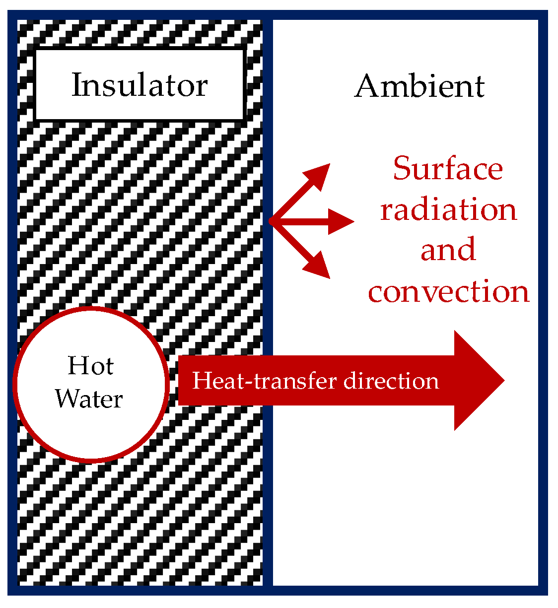
Figure 11 shows the heat transfer from the fluid inside the coil to the ambient air. For the case shown in Figure 11, the heat-exchange area between the coil heater and the insulator was 80% of the whole area of the coil heater. The thermal resistance circuit analysis based on Figure 11 gave the overall heat-transfer coefficient shown in Equation (20). The conductive thermal resistance for the insulator covering the coil heater was based on the shape factor of a row of horizontal cylinders in a semi-infinite medium with an isothermal surface and expressed in Equation (21) [39]. Finally, the overall heat-transfer coefficient for the heat loss from the fluid in the tank to the ambient air is expressed in Equation (24).

$$U_{\mathrm{amb},3}=\frac{1}{\frac{1}{h_{\mathrm{conv},\mathrm{coil}}{A}_{\mathrm{coil},80\%}}+R_{\mathrm{cond},\mathrm{ins}}+U_{\mathrm{ins},\mathrm{s}}}$$

(20)

$$R_{\mathrm{cond},\mathrm{ins}}=\frac{1}{S{F}_{\mathrm{ins}}{k}_{\mathrm{ins}}}$$

(21)

$$S{F}_{\mathrm{ins}}=\frac{2\pi L_{\mathrm{coil}}}{\ln \left[\left(\frac{1}{\pi r_{\mathrm{coil},\mathrm{tube}}}\right)\sinh \frac{2\pi D_c}{l_c}\right]}$$

(22)

$$U_{\mathrm{ins},\mathrm{s}}=\frac{1}{\frac{1}{h_{\mathrm{conv},\mathrm{amb}}{A}_{\mathrm{ins}}}+\frac{1}{h_{\mathrm{rad},\mathrm{amb}}{A}_{\mathrm{ins}}}}$$

(23)

$$U_{\mathrm{amb},2}=\frac{1}{\frac{1}{U_{\mathrm{coil}}}+\frac{1}{U_{\mathrm{amb}}}}$$

(24)

In these equations, $U_{\mathrm{amb},3}$ is the overall heat-transfer coefficient evaluated from the coil heater to the ambient air, $A_{\mathrm{coil},80\%}$ is the heat-exchange area between the coil heater and the tank wall (assumed to be 80% of the whole area of the coil heater), $R_{\mathrm{cond},\mathrm{ins}}$ is the conductive thermal resistance of the insulator covering the coil heater, $S{F}_{\mathrm{ins}}$ is the shape factor for the insulator, $r_{\mathrm{coil},\mathrm{tube}}$ is the radius of the coil tube, $D_c$ is the distance from the center of the coil tube to the surface of the insulator, $l_c$ is the distance between the two centers of the adjacent coil tube, $U_{\mathrm{ins},\mathrm{s}}$ is the overall heat-transfer coefficient at the surface of the insulator, and $U_{\mathrm{amb},2}$ is the overall heat-transfer coefficient for the heat loss from the fluid in the tank to the ambient air.

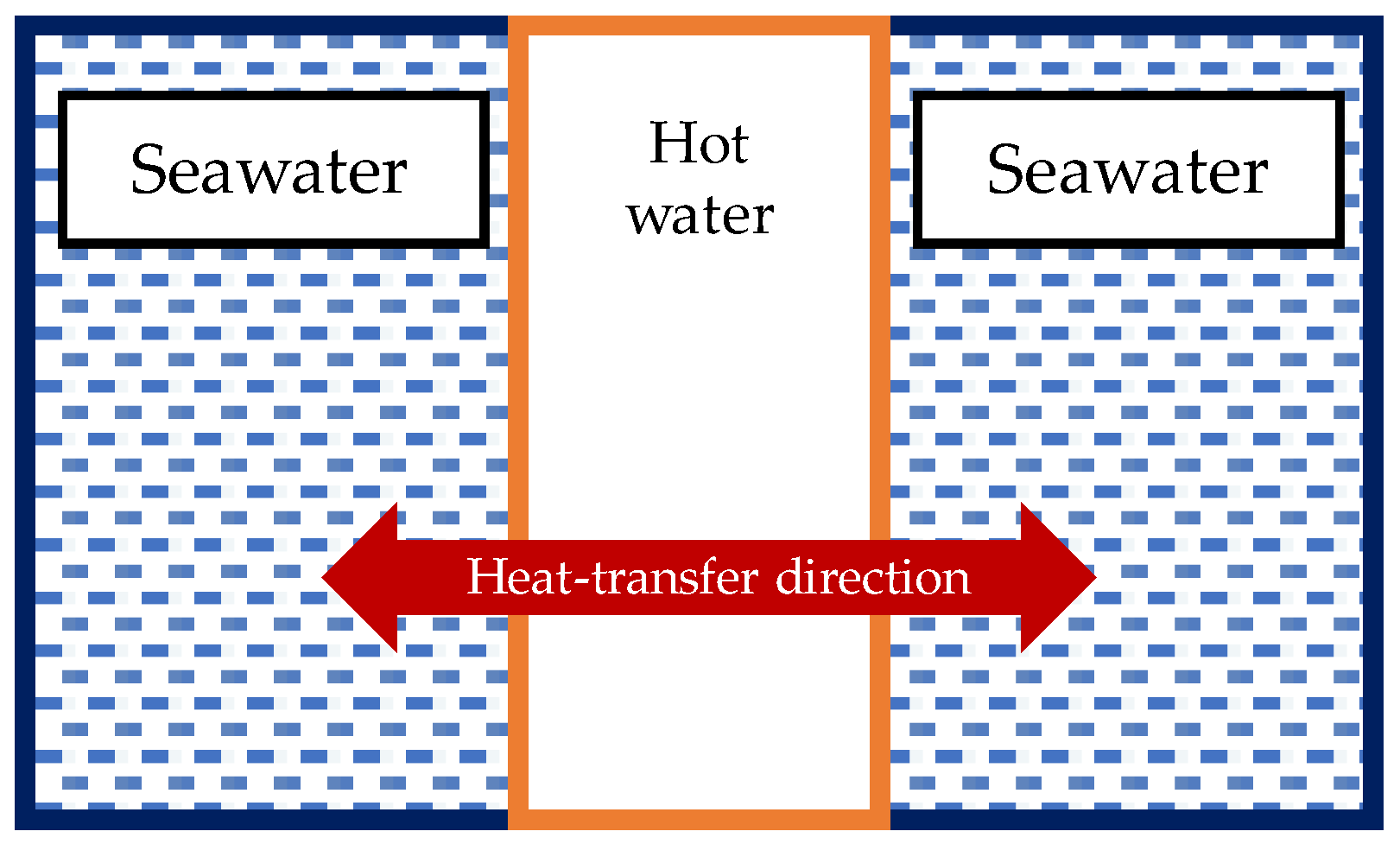
For the vertical bundle heater inside the bioreactor, the internal and external flow of the heat exchanger was considered. Figure 12 illustrates the heat-transfer interaction for the vertical bundle heater inside the reactor. The thermal analysis for the overall heat-transfer coefficient was based on a single tube. The overall heat-transfer coefficient was multiplied by the number of tubes in the bundle to obtain the heat-transfer rate of the heater, as is shown in Equation (25). The internal and external flow Nusselt number correlations for the convective heat-transfer coefficient were calculated by Equations (27) and (28), respectively [35,40]. Equation (27) is applicable for when 0.6 ≤ Pr ≤ 160, Re ≥ 10,000, and (L/D) ≥ 10. The expression in Equations (29)–(31) shows the parameters that need to be calculated in order to use Equation (28) [40]. Equation (29) can only be used when the fluid flow is in natural convection, and 0.01 ≤ Pr ≤ 100.

$$U_{\mathrm{bh}}=\frac{N_{\mathrm{tube}}}{\frac{1}{h_{\mathrm{bh},\mathrm{int}}{A}_{\mathrm{bh},\mathrm{int}}}+R_{\mathrm{cond},\mathrm{bh}}+\frac{1}{h_{\mathrm{bh},\mathrm{ext}}{A}_{\mathrm{bh},\mathrm{ext}}}}$$

(25)

$$R_{\mathrm{cond},\mathrm{bh}}=\ln \left(\frac{D_{\mathrm{o}}/D_{\mathrm{i}}}{2\pi k_{\mathrm{bh}}{L}_{\mathrm{bh},\mathrm{tube}}}\right)$$

(26)

$$N{u}_{\mathrm{L}}=0.023{\mathrm{Re}}_{\mathrm{L}}{}^{0.8}{\mathrm{Pr}}_{\mathrm{w}}{}^{0.4}$$

(27)

$$N{u}_{\mathrm{L}}=N{u}_{\mathrm{fp},\mathrm{L}}\left[1+B{\left({32}^{2}G{r}_{\mathrm{L}}{}^{-0.25}\frac{L_{\mathrm{bh},\mathrm{tube}}}{D_{\mathrm{bh},\mathrm{tube}}}\right)}^C\right]$$

(28)

$$N{u}_{\mathrm{fp},\mathrm{L}}=0.68+\frac{0.67{\mathrm{Ra}}_{\mathrm{L}}{}^{1/4}}{{\left[1+{\left(0.492/{\mathrm{Pr}}_{\mathrm{fl}}\right)}^{{}^{9/16}}\right]}^{4/9}}$$

(29)

$$B=0.0571322+0.20305{\mathrm{Pr}}_{\mathrm{fl}}{}^{-0.43}$$

(30)

$$C=0.9165-0.043{\mathrm{Pr}}_{\mathrm{fl}}{}^{0.5}+0.01333\ln \left({\mathrm{Pr}}_{\mathrm{fl}}\right)+\frac{0.0004809}{{\mathrm{Pr}}_{\mathrm{fl}}}$$

(31)

In these equations, $N_{\mathrm{tube}}$ is the number of tubes in the bundle, $h_{\mathrm{bh},\mathrm{int}}$ is the convective heat-transfer coefficient for the internal flow of the bundle heater tube, $h_{\mathrm{bh},\mathrm{ext}}$ is the convective heat-transfer coefficient for the external flow of the bundle heater tube, $A_{\mathrm{bh},\mathrm{int}}$ is the heat-exchange area for the internal flow of the bundle heater tube, $A_{\mathrm{bh},\mathrm{ext}}$ is the heat-exchange area for the external flow of the bundle heater tube, $D_{\mathrm{i}}$ is the inner diameter of the bundle heater tube, $D_{\mathrm{o}}$ is the outer diameter of the bundle heater tube, $k_{\mathrm{bh}}$ is the thermal conductivity of the bundle heater tube material, $L_{\mathrm{bh},\mathrm{tube}}$ is the length of the bundle heater tube, ${\mathrm{Re}}_{\mathrm{L}}$ is the Reynolds number, and ${\mathrm{Pr}}_{\mathrm{fl}}$ is the Prandtl number of the fluid inside the bioreactor tank.

3. Simulation Algorithm and Parameters

3.1. Simulation Flowchart for the Validation Model and the Biointegrated Gasification Combined Cycle Model

Simulink from MATLAB was utilized for the simulation. The differential equation solver used for high accuracy was the method of solving fourth-order ordinary differential equations. Generally, the calculation for the heat balance was the same for both of the models. Figure 13 illustrates the simulation flowchart for the validation model. This simulation focused on the transient process of heating the fluid inside the tank and the tank’s temperature change. When the simulation was completed, the numerical and experimental results were compared. For the bio-IGCC model, the system had a control process to simulate the filling and emptying of the tanks for the biohydrogen production process, as is shown in Figure 14.

3.2. Simulation Operating Parameters for the Validation Model

Table 1. Operating parameters of the tanks in the validation model.

Parameter	Heat Storage Tank	Feed-Mixing Tank	Bioreactor Tank
Tank capacity (kg)	300	1000	1000
Initial temperature (°C)	72	61	72
Target temperature (°C)	85	80	80
Ambient temperature (°C)	33	33	33
Tank wall thickness (mm)	6	6	6
Tank wall thermal conductivity (W/mK)	52	52	52
Simulation time	6 h 36 min

and

Table 2. Heat-exchanger operating conditions.

	Heat Exchanger
	HST-SB		FMT-HST		BRT-HST
	Cold Side	Hot Side	Cold Side	Hot Side	Cold Side	Hot Side
Tank	Heat storage tank	Steam boiler	Feed-mixing tank	Heat storage tank	Bioreactor tank	Heat storage tank
Mass flow rate (kg/s)	0.29	0.31	0.34	0.59	1.06	0.32
Initial temperature (°C)	64	72	61	64	56	72

present the operating parameters of the validation model. The current model assumed that the fluid’s mass flow rate entered and left the tanks to be heated at the respective tank’s heat exchanger, as is shown in Figure 3.

3.3. Simulation Operating Parameters for the Biointegrated Gasification Combined Cycle Model

An additional process was added to the simulation for the current model in which the fluid was kept inside the feed-mixing tank for a certain amount of time to simulate the condition wherein Thermococcus onnurineus NA1 was cultivated inside the tank. Therefore, a control process of filling and emptying the feed-mixing tank was added to the model. The fluid was kept inside the feed-mixing tank for approximately 5 h intervals.

Table 3. Operating parameters of the feed-mixing and bioreactor tanks in the bio-integrated gasification combined cycle model.

Parameter		Feed-Mixing Tank	Bioreactor Tank
Tank capacity (m3)		1000	1000
Initial volume (m3)		61.1	72.3
Tank volume target (m3)	Upper limit	0.63	33
	Lower limit	0.1	29
Initial temperature (°C)		25	25
Target temperature (°C)		85	80
Tank inner diameter (m)		0.77	2.4
Tank height (m)		1.67	10.37
Tank wall thickness (mm)		6	6
Insulator thickness (mm)		75	75
Inlet mass flow rate (kg/s)		184	5931
Outlet mass flow rate (kg/s)		184	816
Simulation time		24 h

lists the operating parameters for the feed-mixing and bioreactor tanks of the bio-IGCC model.

Table 4. Operating parameters for the shell and tube heat exchanger.

Parameter	Cold Side	Hot Side
Fluid	Seawater	Steam
Mass flow rate (kg/h)	184	21
Inlet temperature (°C)	25	133.51
Outlet temperature (°C)	90	133.37
Heat-exchange area (m2)	0.48

and

Table 5. Operating parameters for the coil heat exchanger for the feed-mixing and bioreactor tanks.

Parameter	Feed-Mixing Tank	Bioreactor Tank
Tube inner diameter (mm)	15.8
Tube outer diameter (mm)	20.3
Fluid	Water
Fluid mass flow rate (kg/h)	2500
Fluid temperature (°C)	90	810
Coil diameter (m)	0.8	2.4
Coil length (m)	17.3	155.0
Coil adjacent distance (mm)	100	295

show the working conditions and operational parameters for the heat exchangers used in the current system. A parametric study was performed to further optimize the current design of the system.

The present study optimized the current system design by determining the new operating volume of the feed-mixing tank that reduced the time for the bioreactor tank to reach the steady-state temperature for hydrogen production. The optimization process focused on the operating parameters without changing the existing physical design of the feed-mixing tank. This optimization parameter was studied by varying the operating volume of the feed-mixing tank, which was chosen because alterations to it caused minimal changes to the current design. The operating volume was varied to obtain the fastest configuration required to reach the targeted steady-state temperature for biohydrogen production in the bioreactor tank (80 °C).

By changing the operating volume, this study aimed to identify whether the steady-state temperature of the bioreactor tank could be reached sooner in the process so that biohydrogen production could start faster. The time required to reach a steady-state temperature is important when a new batch of cultivated Thermococcus onnurineus NA1 is used for the biohydrogen production process. The scale factor coefficient was used to represent the operating volume variations relative to the current operating volume of the feed-mixing tank (

Table 6. Operating volume variations for the optimization of the feed-mixing tank.

	Scale Factor	Volume (m3)
Current volume	1.00	0.630
Increasing volume	1.50	0.945
	1.25	0.788
Decreasing volume	0.75	0.473
	0.50	0.315

).

The evaluation of the effect of varying the feed-mixing tank operating volume was based on how fast the bioreactor tank reached the targeted steady-state temperature (quantified by a parameter called the time constant). The time constant was defined as the length of time it took the system to reach 63% of the steady-state temperature.

4. Results and Discussion

4.1. Lump Capacitance Approach Validation

Based on the tank parameters presented in the previous section, the $Bi$ calculation used the average convective heat-transfer coefficient from the simulated results. Furthermore, additional assumptions needed to be made for the $Bi$ calculation for the tanks in the bio-IGCC model. Since the thickness of the tanks was far less than the diameter of the tanks, the tank walls could be approximated as plane walls.

Table 7. Calculated $Bi$ and parameter value for $Bi$ calculation.

Parameter	Validation Model			Bio-IGCC Model
	Heat Storage Tank	Feed-Mixing Tank	Bioreactor Tank	Feed-Mixing Tank	Bioreactor Tank
Average convective heat-transfer coefficient, ${\mathrm{h}}_{conv,avg}$ (W/m2K)	18.6	17.9	18.7	325.1	368.5
Characteristic length, ${\mathrm{L}}_c$ (mm)	6	6	6	6	6
Tank’s wall thermal conductivity, $k_{wall}$ (W/mK)	52	52	52	52	52
$Bi$	0.002	0.002	0.002	0.040	0.040

lists the parameter values used in the $Bi$ calculation and the calculated $Bi$.

These results demonstrated that the $Bi$ of the tanks in each system was still <0.1, validating the lump capacitance approach. However, it should be noted that the temperature change of the current algorithm used in the developed model was not based on an exponential function since the algorithm was solely based on the heat-transfer equation. Thus, the current model’s accuracy was limited because of the difference in the transient property from the exponential function.

4.2. Simulation Results for the Model Validation

The validation of the developed model was performed by applying similar environmental conditions to the experiment conducted on the basis of the lab-scale biohydrogen production system model. Figure 15 illustrates the comparison between the simulated results and the experimental data. The simulation results indicated that the calculated temperature from the developed model showed good agreement with the experimental data although there were differences in the values throughout the simulation. These differences were due to the instability of the fluid flow rate during the experiment, which affected the heat-transfer process. By contrast, the fluid flow rate in the developed model was set at a constant value.

The relative root-mean-square error (RRMSE) method was used to evaluate the performance of the developed model.

Table 8. RRMSE for the heat storage, feed-mixing, and bioreactor tanks.

Tank	RRMSE (%)
Heat storage tank	1.26
Feed-mixing tank	3.59
Bioreactor tank	1.78

shows the RRMSE for the heat storage, feed-mixing, and bioreactor tanks. The results showed that the error was less than 5% for each tank, indicating that the developed model could predict the biohydrogen production system’s thermal response and validate the developed model within an acceptable limit.

4.3. Simulation Results for the Biointegrated Gasification Combined Cycle Model

Figure 16 illustrates the simulation results for the biohydrogen production process in the bio-IGCC model based on the previously described process flow. The figure demonstrates that there was some inconsistency throughout the simulation for the feed-mixing tank temperature. The temperature instability occurred during the filling and draining process. Based on the presented results, the tank with a lower-volume capacity tended to have its temperature disrupted during filling and draining.

By contrast, the bioreactor tank was heated with an internal and external heat exchanger. The tank’s temperature was much more stable because of the large amount of fluid volume, meaning that the fluid’s heat energy was not easily altered. Additionally, the heat supplied through to the heat-exchanger bundle inside the bioreactor tank ensured that the temperature was maintained at the target value although the tank’s volume was not always constant throughout the process.

Overall, the current system design could meet the thermal requirements of the biohydrogen production process. Hence, the optimization of the current system was based on the heat and mass transfer aspect to ensure that the steady-state temperature for the biohydrogen production process was reached as soon as possible.

Biohydrogen Production System Optimization

The optimization process for the biohydrogen production system was simulated based on varying the volume of the feed-mixing tank. Figure 17 presents the results for the case wherein the operating volume was varied for the feed-mixing and bioreactor tanks. Based on these results, the time for the bioreactor tank to reach a steady-state temperature was reduced when the operating volume of the feed-mixing tank was reduced. Additionally, although the volume was reduced, the bioreactor tank was still able to achieve the targeted steady-state temperature value.

Table 9. Bioreactor tank time constants based on the scale factors of the feed-mixing tank.

Scale Factor	Time Constant (s)
1.00	6099
1.50	5368
1.25	4638
0.75	3907
0.50	3175

lists the results for the time constant from the simulation results. Based on these results, the optimal configurations for the fastest time for the bioreactor tank to reach the steady-state temperature were when the scale factors were 0.75 and 0.50. By reducing the feed-mixing tank operating volume by the scale factors of 0.75 and 0.50, the time constants for the bioreactor tank to reach the steady-state temperature were reduced by 15.76% and 31.54%, respectively, compared with the current operating volume.

5. Conclusions

This study presented the model development for the dynamic simulation of a biohydrogen production system. Two models were simulated, and the same approach was used to analyze both. The first simulated model was validated on the basis of a lab-scale biohydrogen production system, and the second model was based on an IGCC power plant biohydrogen production system. The validation model simulation results showed that the RRMSE for each tank was within an acceptable limit. The RRMSEs for the heat storage, feed-mixing, and bioreactor tanks were 1.26%, 3.59%, and 1.58%, respectively.

As for the IGCC system model, the system’s current design was simulated, and an optimization case study was performed. In the case study, the feed-mixing tank operating volume was varied using the scale factor. The results showed that reducing the operating volume of the feed-mixing tank by the scale factors of 0.75 and 0.50 resulted in better performance than the current operating parameter for volume (resulting in a decrease in the starting time of the biohydrogen production process by 15.76% and 31.54%, respectively). This volume reduction occurred under the same conditions as the current operating parameter.

References

1. Gräbner, M. Industrial Coal Gasification Technologies Covering Baseline and High-Ash Coal; Gräbner, M., Ed.; Wiley-VCH Verlag GmbH & Co. KGaA: Weinheim, Germany, 2014; ISBN 9783527336913. [Google Scholar]
2. Cormos, C.C. Evaluation of Energy Integration Aspects for IGCC-Based Hydrogen and Electricity Co-Production with Carbon Capture and Storage. Int. J. Hydrogen Energy 2010, 35, 7485–7497. [Google Scholar] [CrossRef]
3. Johnsson, F.; Odenberger, M.; Göransson, L. Challenges to Integrate CCS into Low Carbon Electricity Markets. Energy Procedia 2014, 63, 7485–7493. [Google Scholar] [CrossRef] [Green Version]
4. Cormos, C.C. Hydrogen and Power Co-Generation Based on Coal and Biomass/Solid Wastes Co-Gasification with Carbon Capture and Storage. Int. J. Hydrogen Energy 2012, 37, 5637–5648. [Google Scholar] [CrossRef]
5. Cormos, A.M.; Cormos, C.C. Techno-Economic Assessment of Combined Hydrogen & Power Co-Generation with Carbon Capture: The Case of Coal Gasification. Appl. Therm. Eng. 2019, 147, 29–39. [Google Scholar] [CrossRef]
6. Giuliano, A.; Poletto, M.; Barletta, D. Pure Hydrogen Co-Production by Membrane Technology in an IGCC Power Plant with Carbon Capture. Int. J. Hydrogen Energy 2018, 43, 19279–19292. [Google Scholar] [CrossRef]
7. Kreutz, T.; Williams, R.; Consonni, S.; Chiesa, P. Co-Production of Hydrogen, Electricity and CO2 from Coal with Commercially Ready Technology. Part B: Economic Analysis. Int. J. Hydrogen Energy 2005, 30, 769–784. [Google Scholar] [CrossRef]
8. Starr, F.; Tzimas, E.; Peteves, S. Critical Factors in the Design, Operation and Economics of Coal Gasification Plants: The Case of the Flexible Co-Production of Hydrogen and Electricity. Int. J. Hydrogen Energy 2007, 32, 1477–1485. [Google Scholar] [CrossRef]
9. Szima, S.; del Pozo, C.A.; Cloete, S.; Chiesa, P.; Jiménez Alvaro, Á.; Cormos, A.M.; Amini, S. Finding Synergy between Renewables and Coal: Flexible Power and Hydrogen Production from Advanced IGCC Plants with Integrated CO2 Capture. Energy Convers. Manag. 2021, 231, 113866. [Google Scholar] [CrossRef]
10. Argun, H.; Kargi, F. Bio-Hydrogen Production by Different Operational Modes of Dark and Photo-Fermentation: An Overview. Int. J. Hydrogen Energy 2011, 36, 7443–7459. [Google Scholar] [CrossRef]
11. Arimi, M.M.; Knodel, J.; Kiprop, A.; Namango, S.S.; Zhang, Y.; Geißen, S.U. Strategies for Improvement of Biohydrogen Production from Organic-Rich Wastewater: A Review. Biomass Bioenergy 2015, 75, 101–118. [Google Scholar] [CrossRef]
12. Levin, D.B.; Pitt, L.; Love, M. Biohydrogen Production: Prospects and Limitations to Practical Application. Int. J. Hydrogen Energy 2004, 29, 173–185. [Google Scholar] [CrossRef]
13. Kothari, R.; Singh, D.P.; Tyagi, V.V.; Tyagi, S.K. Fermentative Hydrogen Production—An Alternative Clean Energy Source. Renew. Sustain. Energy Rev. 2012, 16, 2337–2346. [Google Scholar] [CrossRef]
14. Srivastava, R.K.; Shetti, N.P.; Reddy, K.R.; Aminabhavi, T.M. Biofuels, Biodiesel and Biohydrogen Production Using Bioprocesses. A Review. Environ. Chem. Lett. 2020, 18, 1049–1072. [Google Scholar] [CrossRef]
15. Park, J.H.; Chandrasekhar, K.; Jeon, B.H.; Jang, M.; Liu, Y.; Kim, S.H. State-of-the-Art Technologies for Continuous High-Rate Biohydrogen Production. Bioresour. Technol. 2021, 320, 124304. [Google Scholar] [CrossRef]
16. Mirza, S.S.; Qazi, J.I.; Liang, Y.; Chen, S. Growth Characteristics and Photofermentative Biohydrogen Production Potential of Purple Non Sulfur Bacteria from Sugar Cane Bagasse. Fuel 2019, 255, 115805. [Google Scholar] [CrossRef]
17. Lu, C.; Zhang, H.; Zhang, Q.; Chu, C.Y.; Tahir, N.; Ge, X.; Jing, Y.; Hu, J.; Li, Y.; Zhang, Y.; et al. An Automated Control System for Pilot-Scale Biohydrogen Production: Design, Operation and Validation. Int. J. Hydrogen Energy 2020, 45, 3795–3806. [Google Scholar] [CrossRef]
18. Rupprecht, J.; Hankamer, B.; Mussgnug, J.H.; Ananyev, G.; Dismukes, C.; Kruse, O. Perspectives and Advances of Biological H2 Production in Microorganisms. Appl. Microbiol. Biotechnol. 2006, 72, 442–449. [Google Scholar] [CrossRef]
19. Prabakar, D.; Manimudi, V.T.; Suvetha, K.S.; Sampath, S.; Mahapatra, D.M.; Rajendran, K.; Pugazhendhi, A. Advanced Biohydrogen Production Using Pretreated Industrial Waste: Outlook and Prospects. Renew. Sustain. Energy Rev. 2018, 96, 306–324. [Google Scholar] [CrossRef]
20. Kumar, G.; Sivagurunathan, P.; Pugazhendhi, A.; Thi, N.B.D.; Zhen, G.; Chandrasekhar, K.; Kadier, A. A Comprehensive Overview on Light Independent Fermentative Hydrogen Production from Wastewater Feedstock and Possible Integrative Options. Energy Convers. Manag. 2017, 141, 390–402. [Google Scholar] [CrossRef]
21. Sathyaprakasan, P.; Kannan, G. Economics of Bio-Hydrogen Production. Int. J. Environ. Sci. Dev. 2015, 6, 352–356. [Google Scholar] [CrossRef] [Green Version]
22. Ding, C.; Yang, K.L.; He, J. Biological and Fermentative Production of Hydrogen. In Handbook of Biofuels Production: Processes and Technologies, 2nd ed.; Woodhead Publishing: Sawston, UK, 2016; pp. 303–333. [Google Scholar] [CrossRef]
23. Sarangi, P.K.; Nanda, S. Biohydrogen Production through Dark Fermentation. Chem. Eng. Technol. 2020, 43, 601–612. [Google Scholar] [CrossRef]
24. Lee, J.; Seol, E.; Kaur, G.; Oh, Y.; Park, S. Hydrogen Production from C1 Compounds by a Novel Marine Hyperthermophilic Archaeon Thermococcus Onnurineus NA1. Int. J. Hydrogen Energy 2012, 37, 11113–11121. [Google Scholar] [CrossRef]
25. Kim, M.S.; Bae, S.S.; Kim, Y.J.; Kim, T.W.; Lim, J.K.; Lee, S.H.; Choi, A.R.; Jeon, J.H.; Lee, J.H.; Lee, H.S.; et al. Co-Dependent H2 Production by Genetically Engineered Thermococcus Onnurineus NA1. Appl. Environ. Microbiol. 2013, 79, 2048–2053. [Google Scholar] [CrossRef] [Green Version]
26. Sivagurunathan, P.; Anburajan, P.; Park, J.H.; Kumar, G.; Park, H.D.; Kim, S.H. Mesophilic Biogenic H2 Production Using Galactose in a Fixed Bed Reactor. Int. J. Hydrogen Energy 2017, 42, 3658–3666. [Google Scholar] [CrossRef]
27. Park, J.H.; Anburajan, P.; Kumar, G.; Park, H.D.; Kim, S.H. Biohydrogen Production Integrated with an External Dynamic Membrane: A Novel Approach. Int. J. Hydrogen Energy 2017, 42, 27543–27549. [Google Scholar] [CrossRef]
28. Karapinar, I.; Gokfiliz Yildiz, P.; Pamuk, R.T.; Karaosmanoglu Gorgec, F. The Effect of Hydraulic Retention Time on Thermophilic Dark Fermentative Biohydrogen Production in the Continuously Operated Packed Bed Bioreactor. Int. J. Hydrogen Energy 2020, 45, 3524–3531. [Google Scholar] [CrossRef]
29. Su, C.; Liu, Y.; Yang, X.; Li, H. Effect of Hydraulic Retention Time on Biohydrogen Production from Glucose in an Internal Circulation Reactor. Energy Fuels 2020, 34, 3244–3249. [Google Scholar] [CrossRef]
30. Kim, H.J.; Kim, S.Y.; Ahn, J. Dynamic Thermal Design of a 1-Ton Class Bio-Hydrogen Production System Simulator Using Industrial Waste Heat and by-Products. Korean J. Air-Cond. Refrig. Eng. 2017, 29, 259–268. [Google Scholar]
31. Rittmann, S.K.R.; Sook, H.; Kyu, J.; Wan, T.; Lee, J.; Gyun, S. One-Carbon Substrate-Based Biohydrogen Production: Microbes, Mechanism, and Productivity. Biotechnol. Adv. 2015, 33, 165–177. [Google Scholar] [CrossRef]
32. Lee, S.; Park, J.; Lee, C.; Lee, D.; Kim, H.; Won, H.; Kim, S.; Ryi, S. H2 Recovery and CO2 Capture after Water-Gas Shift Reactor Using Synthesis Gas from Coal Gasification. Energy 2014, 66, 635–642. [Google Scholar] [CrossRef]
33. Kim, M.S.; Fitriana, H.N.; Kim, T.W.; Kang, S.G.; Jeon, S.G.; Chung, S.H.; Park, G.W.; Na, J.G. Enhancement of the Hydrogen Productivity in Microbial Water Gas Shift Reaction by Thermococcus Onnurineus NA1 Using a Pressurized Bioreactor. Int. J. Hydrogen Energy 2017, 42, 27593–27599. [Google Scholar] [CrossRef]
34. Novotny, V.; Vitvarova, M.; Kolovratnik, M.; Hrdina, Z. Minimizing the Energy and Economic Penalty of CCS Power Plants through Waste Heat Recovery Systems. Energy Procedia 2017, 108, 10–17. [Google Scholar] [CrossRef]
35. Incropera, F.P.; De Witt, D.P.; Bergman, T.L.; Lavine, A.S. Fundamentals of Heat and Mass Transfer, 7th ed.; John Wiley & Sons, Inc.: Hoboken, NJ, USA, 2011; ISBN 9780470646151. [Google Scholar]
36. Hexact|Heat Exchanger Design Software|Danfoss. Available online: https://www.danfoss.com/en/service-and-support/downloads/dcs/hexact/#tab-overview (accessed on 26 October 2021).
37. Manlapaz, R.L.; Churchill, S.W. Fully Developed Laminar Convection from a Helical Coil. Chem. Eng. Commun. 1981, 9, 185–200. [Google Scholar] [CrossRef]
38. Morrison, G.L. Simulation of Packaged Solar Heat-Pump Water Heaters. Sol. Energy 1994, 53, 249–257. [Google Scholar] [CrossRef]
39. Holman, J.P. Heat Transfer, 10th ed.; McGraw-Hill: New York, NY, USA, 2010. [Google Scholar]
40. Boetcher, S.K.S. Natural Convection from Circular Cylinders; Springer: New York, NY, USA, 2014; ISBN 9783319081311. [Google Scholar]
Figure 1. Three-dimensional, computer-aided design drawing of the lab-scale biohydrogen production system setup.
Energies 15 02976 g001
Figure 2. The facility of the lab-scale bio-hydrogen production system setup.
Energies 15 02976 g002
Figure 3. Schematic drawing of the lab-scale biohydrogen production system.
Energies 15 02976 g003
Figure 4. IGCC power plant biohydrogen production system.
Energies 15 02976 g004
Figure 5. Steam boiler temperature profile.
Energies 15 02976 g005
Figure 6. Each tank’s heat and mass transfer interaction in the lab-scale biohydrogen production system.
Energies 15 02976 g006
Figure 7. Heat transfer from the fluid inside the tank to the ambient air.
Energies 15 02976 g007
Figure 8. Heat and mass interaction for the (a) feed-mixing tank and (b) bioreactor tank in the integrated gasification combined cycle biohydrogen production system.
Energies 15 02976 g008
Figure 9. Directions of heat transfer between the coil heater, the fluid in the tanks, and the ambient air.
Energies 15 02976 g009
Figure 10. Heat-transfer direction from the water inside the coil heater to the fluid inside the tank.
Energies 15 02976 g010
Figure 11. Heat-transfer direction from the water inside the coil heater to the ambient air.
Energies 15 02976 g011
Figure 12. Heat-transfer interaction for the vertical bundle heater.
Energies 15 02976 g012
Figure 13. Simulation flowchart for the validation model.
Energies 15 02976 g013
Figure 14. Simulation flowchart for the bio-integrated gasification combined cycle model.
Energies 15 02976 g014
Figure 15. Comparison between the simulated results and the experimental data for the (a) heat storage tank, (b) feed-mixing tank, and (c) bioreactor tank.
Energies 15 02976 g015
Figure 16. Simulation results for temperature and volume versus time of the (a) feed-mixing tank and (b) bioreactor tank.
Energies 15 02976 g016
Figure 17. Simulation results for the (a) feed-mixing tank volume versus time, (b) feed-mixing tank temperature versus time, (c) bioreactor tank temperature versus time, and (d) bioreactor tank volume versus time.
Energies 15 02976 g017aEnergies 15 02976 g017b