
A New Wind Speed Scenario Generation Method Based on Principal Component and R-Vine Copula Theories

 ,
, 
 ,
,
Abstract
:1. Introduction
2. Principal Component and Vine Copula Theories
2.1. Principal Component Generation Process
- Centralized input data:
- Calculation of the covariance matrix of the input data:
- Calculation of eigenvalue vector and eigenvector matrix of matrix :
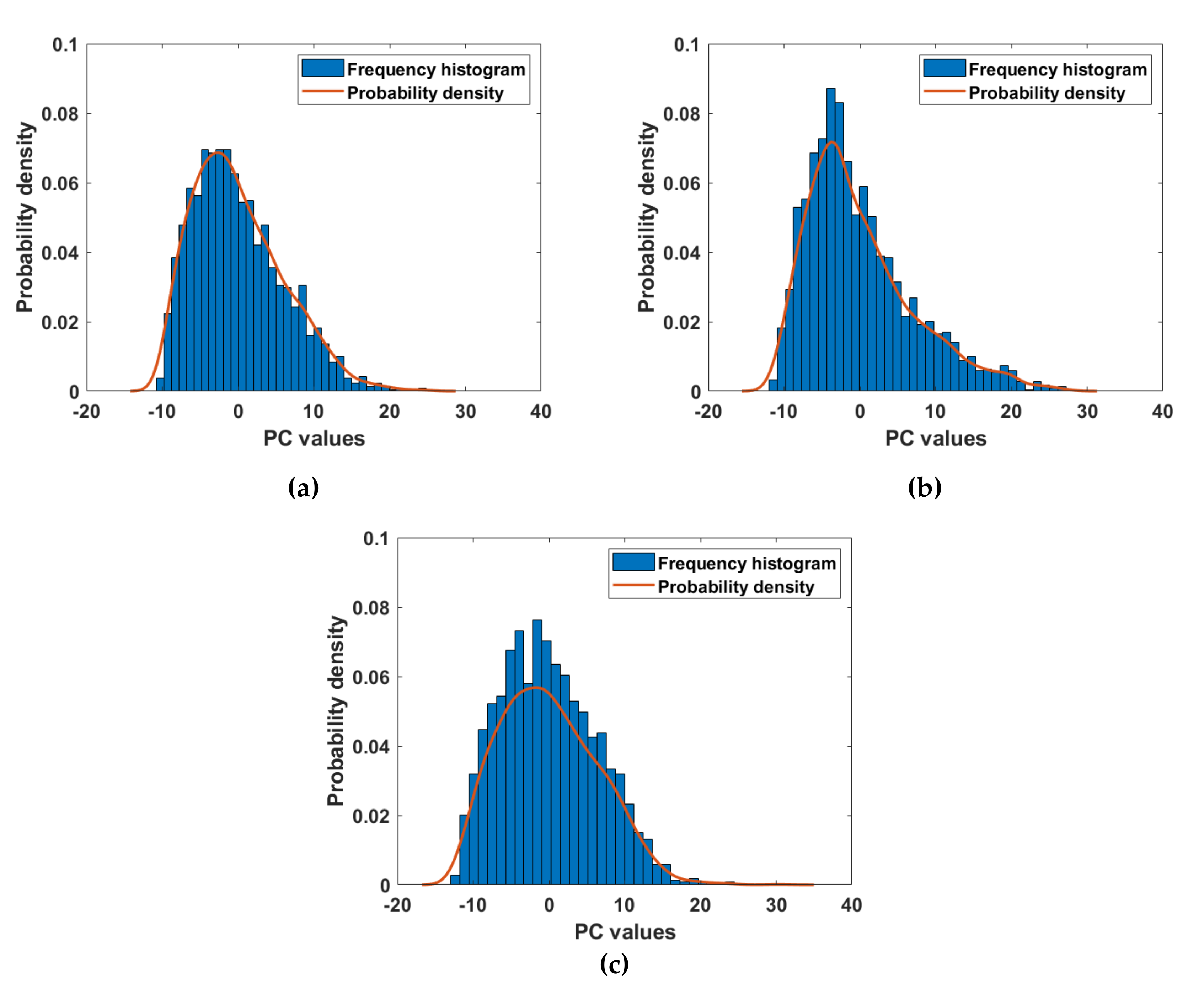
- Calculation of principal components:Each row in is a PC, and the order of PC is the number of the row it is in.
2.2. Vine Copula Theory
2.2.1. Copula Theory
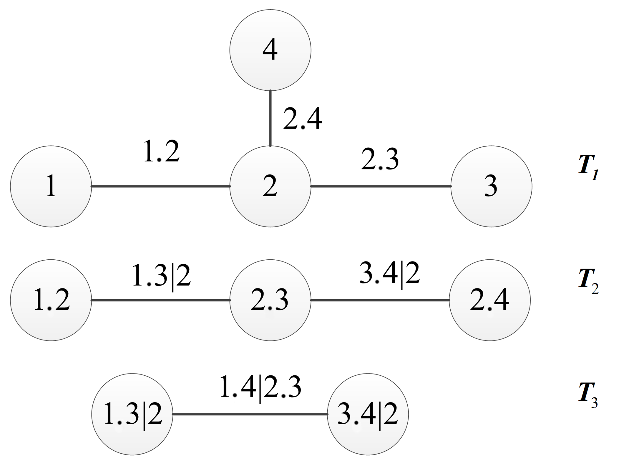
2.2.2. R-Vine Copula
3. Formulation of Wind Speed Scenarios
3.1. Reification of the Structure of the R-Vine Copula Model
3.2. Procedure of Scenario Generation Method
| Algorithm 1 Mixed method to generate wind speed scenarios based on PC and R-vine copula theories. |
| Input: Historical wind speed of wind farms in years. |
| Output: Wind speed scenarios of wind farms. |
| 1: for do |
| 2: Divide the samples of wind farm into 24 sample sets by time . |
| 3: end for |
| 4: for do |
| 5: Apply PC theory to the matrix consisting of sample sets of wind farms at the hour. |
| 6: Transform the values of each PC into CDF values using KDE. |
| 7: end for |
| 8: for do |
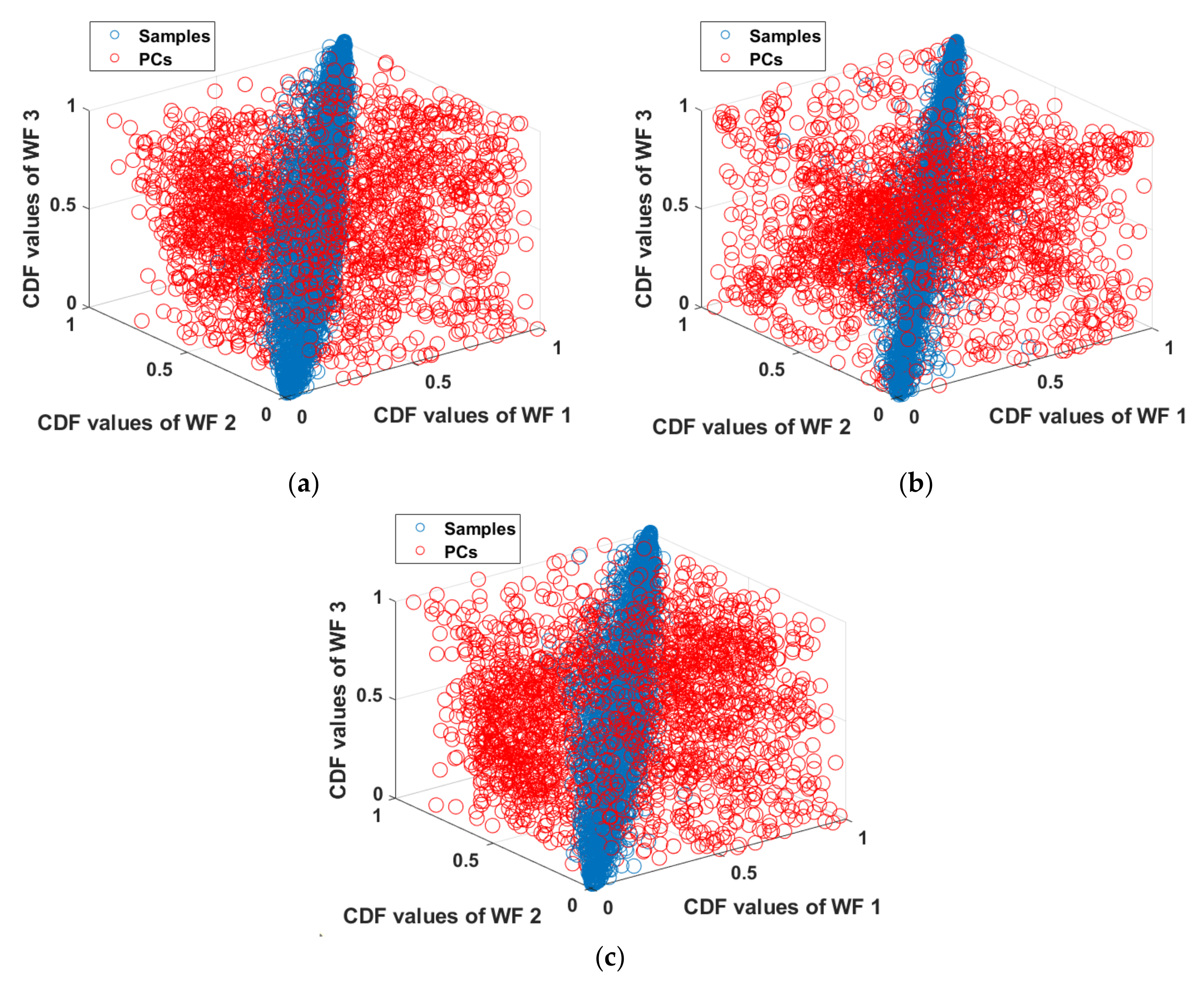
| 9: Apply the R-vine copula model to generate PC scenarios according to the matrix consisting of the PCs of each hour. |
| 10: end for |
| 11: for do |
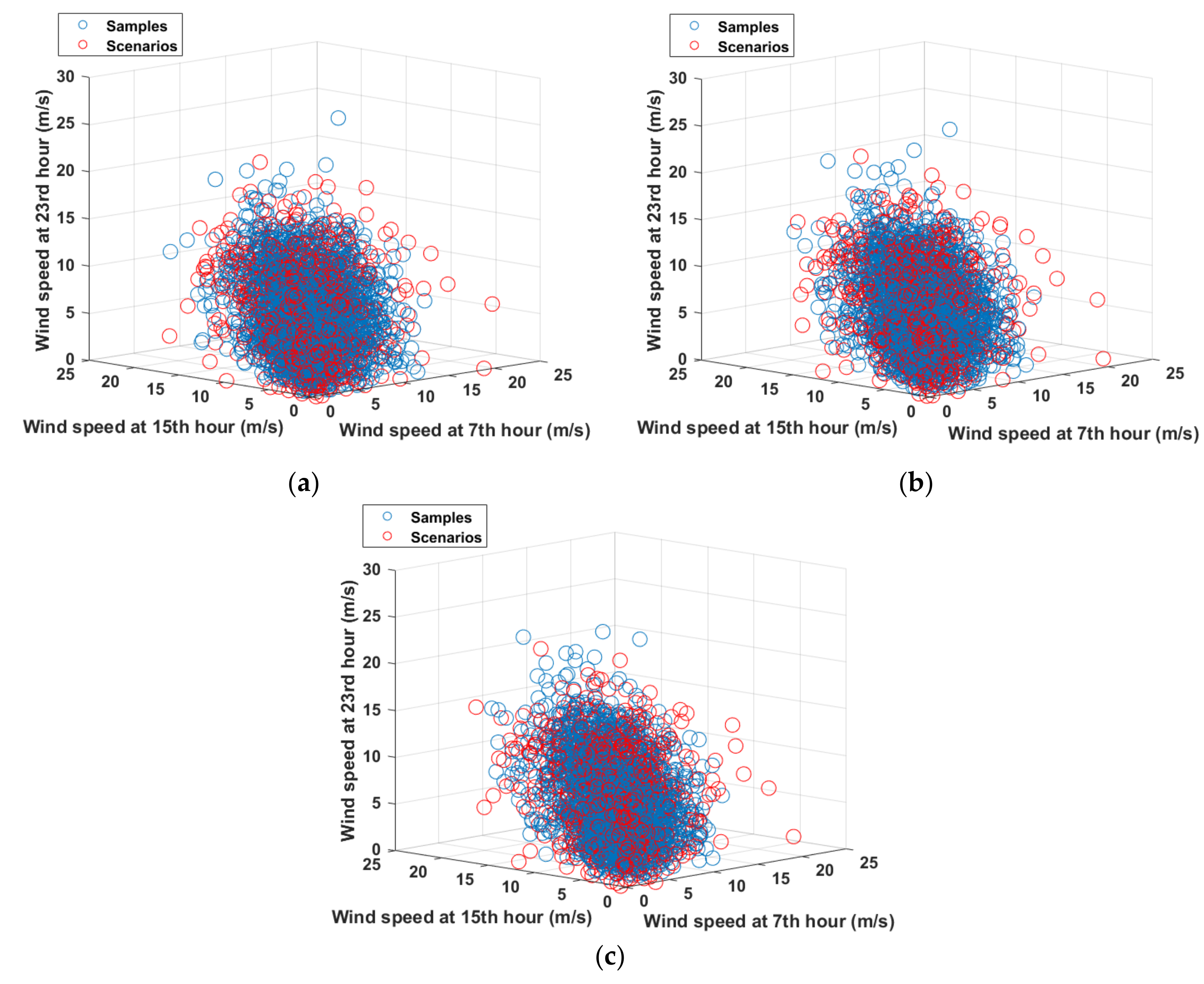
| 12: Restore the generated PCs of the hour to wind speed scenarios by data reconstruction of PC theory and the inverse transformation of the kernel density function. |
| 13: end for |
4. Results and Analysis
4.1. Data Sources
4.2. Evaluation of the Process for Generating Wind Speed Scenarios
4.3. Comparison of Typical Scenario Generation Methods
- 5.
- Output-based evaluation
- 6.
- Distribution-based evaluation
- 7.
- Event-based evaluation
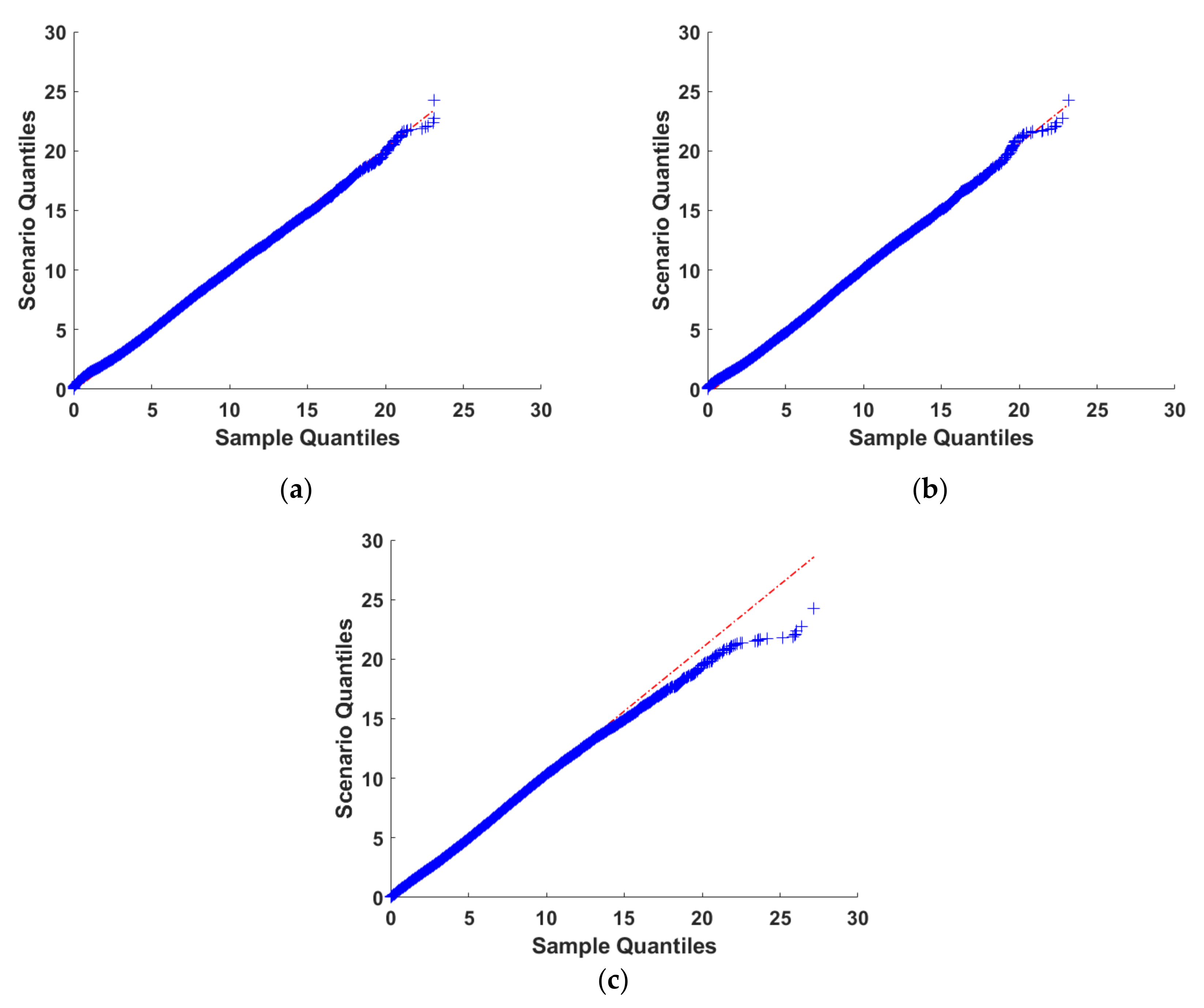
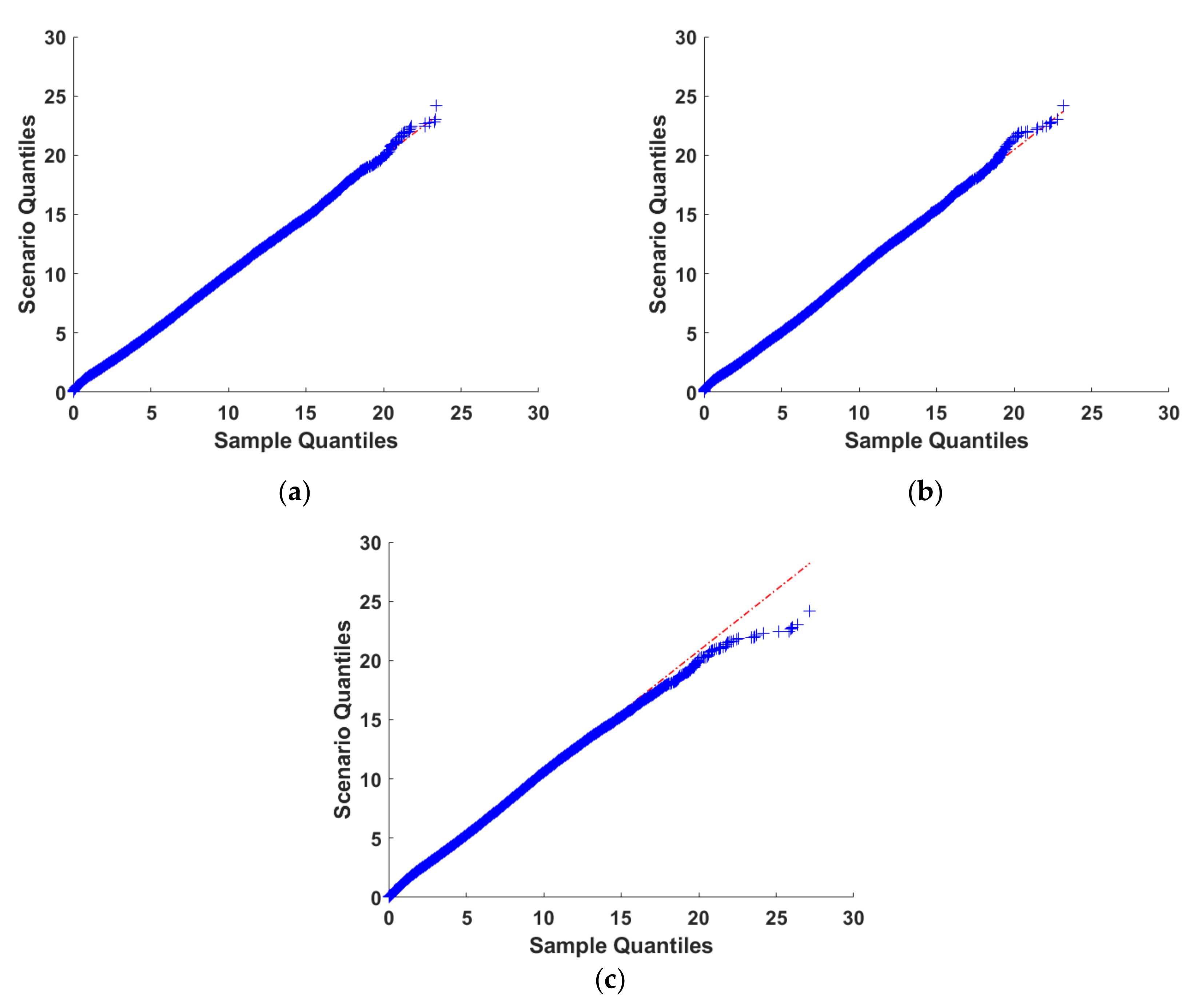
4.4. Comparison of Several Vine Structure Models
5. Conclusions
Author Contributions
Funding
Institutional Review Board Statement
Informed Consent Statement
Data Availability Statement
Conflicts of Interest
References
- Goh, H.H.; He, R.; Zhang, D.; Liu, H.; Dai, W.; Lim, C.S.; Kurniawan, T.A.; Teo, K.T.K.; Goh, K.C. A multimodal approach to chaotic renewable energy prediction using meteorological and historical information. Appl. Soft Comput. 2022, 118, 108487. [Google Scholar] [CrossRef]
- Sahragard, A.; Falaghi, H.; Farhadi, M.; Mosavi, A.; Estebsari, A. Generation Expansion Planning in the Presence of Wind Power Plants Using a Genetic Algorithm Model. Electronics 2020, 9, 1143. [Google Scholar] [CrossRef]
- Band, S.S.; Bateni, S.M.; Almazroui, M.; Sajjadi, S.; Chau, K.-w.; Mosavi, A. Evaluating the potential of offshore wind energy in the Gulf of Oman using the MENA-CORDEX wind speed data simulations. Eng. Appl. Comput. Fluid Mech. 2021, 15, 613–626. [Google Scholar] [CrossRef]
- D’Amico, G.; Petroni, F.; Prattico, F. First and second order semi-Markov chains for wind speed modeling. Phys. A Stat. Mech. Its Appl. 2013, 392, 1194–1201. [Google Scholar] [CrossRef] [Green Version]
- Chen, J.; Rabiti, C. Synthetic wind speed scenarios generation for probabilistic analysis of hybrid energy systems. Energy 2017, 120, 507–517. [Google Scholar] [CrossRef] [Green Version]
- Sim, S.K.; Maass, P.; Lind, P.J.E. Wind Speed Modeling by Nested ARIMA Processes. Energies 2018, 12, 69. [Google Scholar] [CrossRef] [Green Version]
- Sun, W.; Zamani, M.; Zhang, H.T.; Li, Y. Probabilistic Optimal Power Flow With Correlated Wind Power Uncertainty via Markov Chain Quasi-Monte-Carlo Sampling. IEEE Trans. Ind. Inform. 2019, 15, 6058–6069. [Google Scholar] [CrossRef]
- Morales, J.M.; Mínguez, R.; Conejo, A.J. A methodology to generate statistically dependent wind speed scenarios. Appl. Energy 2010, 87, 843–855. [Google Scholar] [CrossRef]
- Abedi, A.; Rahimiyan, M. Day-ahead energy and reserve scheduling under correlated wind power production. Int. J. Electr. Power Energy Syst. 2020, 120, 105931. [Google Scholar] [CrossRef]
- Le, D.D.; Gross, G.; Berizzi, A. Probabilistic Modeling of Multisite Wind Farm Production for Scenario-Based Applications. IEEE Trans. Sustain. Energy 2015, 6, 748–758. [Google Scholar] [CrossRef] [Green Version]
- Chen, Y.; Wang, Y.; Kirschen, D.; Zhang, B. Model-Free Renewable Scenario Generation Using Generative Adversarial Networks. IEEE Trans. Power Syst. 2018, 33, 3265–3275. [Google Scholar] [CrossRef] [Green Version]
- Zhang, Y.; Ai, Q.; Xiao, F.; Hao, R.; Lu, T. Typical wind power scenario generation for multiple wind farms using conditional improved Wasserstein generative adversarial network. Int. J. Electr. Power Energy Syst. 2020, 114, 105388. [Google Scholar] [CrossRef]
- Jiang, C.; Mao, Y.; Chai, Y.; Yu, M.; Tao, S. Scenario Generation for Wind Power Using Improved Generative Adversarial Networks. IEEE Access 2018, 6, 62193–62203. [Google Scholar] [CrossRef]
- Qiao, J.; Pu, T.; Wang, X. Renewable scenario generation using controllable generative adversarial networks with transparent latent space. CSEE J. Power Energy Syst. 2021, 7, 66–77. [Google Scholar]
- Liang, J.; Tang, W. Sequence Generative Adversarial Networks for Wind Power Scenario Generation. IEEE J. Sel. Areas Commun. 2020, 38, 110–118. [Google Scholar] [CrossRef]
- Haghi, H.V.; Lotfifard, S. Spatiotemporal Modeling of Wind Generation for Optimal Energy Storage Sizing. IEEE Trans. Sustain. Energy 2015, 6, 113–121. [Google Scholar] [CrossRef]
- Becker, R. Generation of Time-Coupled Wind Power Infeed Scenarios Using Pair-Copula Construction. IEEE Trans. Sustain. Energy 2018, 9, 1298–1306. [Google Scholar] [CrossRef]
- Lin, Z.; Chen, H.; Wu, Q.; Huang, J.; Li, M.; Ji, T. A data-adaptive robust unit commitment model considering high penetration of wind power generation and its enhanced uncertainty set. Int. J. Electr. Power Energy Syst. 2021, 129, 106797. [Google Scholar] [CrossRef]
- Borujeni, M.S.; Foroud, A.A.; Dideban, A. Wind speed scenario generation based on dependency structure analysis. J. Wind Eng. Ind. Aerodyn. 2018, 172, 453–465. [Google Scholar] [CrossRef]
- Eryilmaz, S.; Kan, C. Reliability based modeling and analysis for a wind power system integrated by two wind farms considering wind speed dependence. Reliab. Eng. Syst. Saf. 2020, 203, 107077. [Google Scholar] [CrossRef]
- Li, M.S.; Lin, Z.J.; Ji, T.Y.; Wu, Q.H. Risk constrained stochastic economic dispatch considering dependence of multiple wind farms using pair-copula. Appl. Energy 2018, 226, 967–978. [Google Scholar] [CrossRef]
- Deng, J.; Li, H.; Hu, J.; Liu, Z. A new wind speed scenario generation method based on spatiotemporal dependency structure. Renew. Energy 2021, 163, 1951–1962. [Google Scholar] [CrossRef]
- Qiu, Y.; Li, Q.; Pan, Y.; Yang, H.; Chen, W. A scenario generation method based on the mixture vine copula and its application in the power system with wind/hydrogen production. Int. J. Hydrogen Energy 2019, 44, 5162–5170. [Google Scholar] [CrossRef]
- Xu, J.; Wu, W.; Wang, K.; Li, G. C-Vine pair copula based wind power correlation modelling in probabilistic small signal stability analysis. IEEE CAA J. Autom. Sin. 2020, 7, 1154–1160. [Google Scholar] [CrossRef]
- Henderson, S.B.; Shahirinia, A.H.; Tavakoli Bina, M. Bayesian estimation of copula parameters for wind speed models of dependence. IET Renew. Power Gener. 2021, 15, 3823–3831. [Google Scholar] [CrossRef]
- Wang, C.; Liang, Z.; Liang, J.; Teng, Q.; Dong, X.; Wang, Z. Modeling the temporal correlation of hourly day-ahead short-term wind power forecast error for optimal sizing energy storage system. Int. J. Electr. Power Energy Syst. 2018, 98, 373–381. [Google Scholar] [CrossRef]
- Li, L.; Miao, S.; Tu, Q.; Duan, S.; Li, Y.; Han, J. Dynamic dependence modelling of wind power uncertainty considering heteroscedastic effect. Int. J. Electr. Power Energy Syst. 2020, 116, 105556. [Google Scholar] [CrossRef]
- Philippe, W.P.J.; Zhang, S.; Eftekharnejad, S.; Ghosh, P.K.; Varshney, P.K. Mixed Copula-Based Uncertainty Modeling of Hourly Wind Farm Production for Power System Operational Planning Studies. IEEE Access 2020, 8, 138569–138583. [Google Scholar] [CrossRef]
- Wang, Z.; Wang, W.; Liu, C.; Wang, Z.; Hou, Y. Probabilistic Forecast for Multiple Wind Farms Based on Regular Vine Copulas. IEEE Trans. Power Syst. 2018, 33, 578–589. [Google Scholar] [CrossRef]
- Wang, Z.; Wang, W.; Liu, C.; Wang, B. Forecasted Scenarios of Regional Wind Farms Based on Regular Vine Copulas. J. Mod. Power Syst. Clean Energy 2020, 8, 77–85. [Google Scholar] [CrossRef]
- Xiao, Q.; Zhou, S. Probabilistic power flow computation considering correlated wind speeds. Appl. Energy 2018, 231, 677–685. [Google Scholar] [CrossRef]
- Zhou, S.; Xiao, Q.; Wu, L. Probabilistic power flow analysis with correlated wind speeds. Renew. Energy 2020, 145, 2169–2177. [Google Scholar] [CrossRef]
- Xiao, Q.; Zhou, S.; Xiao, H. Probabilistic optimal power flow analysis incorporating correlated wind sources. Int. Trans. Electr. Energy Syst. 2020, 30, e12441. [Google Scholar] [CrossRef]
- Dißmann, J.; Brechmann, E.C.; Czado, C.; Kurowicka, D. Selecting and estimating regular vine copulae and application to financial returns. Comput. Stat. Data Anal. 2013, 59, 52–69. [Google Scholar] [CrossRef] [Green Version]
- NREL. Wind Speed Dataset. Available online: https://maps.nrel.gov/wind-prospector/ (accessed on 14 January 2022).
- Li, J.; Zhou, J.; Chen, B. Review of wind power scenario generation methods for optimal operation of renewable energy systems. Appl. Energy 2020, 280, 115992. [Google Scholar] [CrossRef]


| PC-R-Vine | PCA-ARMA | HMCM | |
|---|---|---|---|
| 0.0143 | 0.0701 | 0.0175 | |
| 0.0287 | 0.0435 | 0.0224 | |
| 0.0983 | 0.4272 | 0.3807 | |
| 0.0411 | 0.1981 | 0.2009 | |
| 0.0421 | 0.0844 | 0.3945 | |
| 0.0019 | 0.0088 | 0.0033 |
| PC-R-Vine | PCA-ARMA | HMCM | |
|---|---|---|---|
| UPM (%) | 0.22 | 0.46 | 0.49 |
| R-Vine | C-Vine | D-Vine | |
|---|---|---|---|
| 0.0143 | 0.0308 | 0.0315 | |
| 0.0287 | 0.0568 | 0.0559 | |
| 0.0983 | 0.0944 | 0.0905 | |
| 0.0411 | 0.0670 | 0.0521 | |
| 0.0421 | 0.0367 | 0.0371 | |
| 0.0019 | 0.0023 | 0.0021 | |
| UPM (%) | 0.22 | 0.29 | 0.29 |
Publisher’s Note: MDPI stays neutral with regard to jurisdictional claims in published maps and institutional affiliations. |
© 2022 by the authors. Licensee MDPI, Basel, Switzerland. This article is an open access article distributed under the terms and conditions of the Creative Commons Attribution (CC BY) license (https://creativecommons.org/licenses/by/4.0/).
Share and Cite
Goh, H.H.; Peng, G.; Zhang, D.; Dai, W.; Kurniawan, T.A.; Goh, K.C.; Cham, C.L. A New Wind Speed Scenario Generation Method Based on Principal Component and R-Vine Copula Theories. Energies 2022, 15, 2698. https://doi.org/10.3390/en15072698
Goh HH, Peng G, Zhang D, Dai W, Kurniawan TA, Goh KC, Cham CL. A New Wind Speed Scenario Generation Method Based on Principal Component and R-Vine Copula Theories. Energies. 2022; 15(7):2698. https://doi.org/10.3390/en15072698
Chicago/Turabian StyleGoh, Hui Hwang, Gumeng Peng, Dongdong Zhang, Wei Dai, Tonni Agustiono Kurniawan, Kai Chen Goh, and Chin Leei Cham. 2022. "A New Wind Speed Scenario Generation Method Based on Principal Component and R-Vine Copula Theories" Energies 15, no. 7: 2698. https://doi.org/10.3390/en15072698
APA StyleGoh, H. H., Peng, G., Zhang, D., Dai, W., Kurniawan, T. A., Goh, K. C., & Cham, C. L. (2022). A New Wind Speed Scenario Generation Method Based on Principal Component and R-Vine Copula Theories. Energies, 15(7), 2698. https://doi.org/10.3390/en15072698