CO₂ Emission Factors and Carbon Losses for Off-Road Mining Trucks

Abstract

There are myriad questions that remain to be answered in greenhouse gas (GHG) emissions trading. This article addresses carbon dioxide (CO₂) emission factors and carbon losses from heavy equipment that is used to transport ores. Differences occurred between the Intergovernmental Panel for Climate Change (IPCC) emission factor and those that were obtained by considering incomplete combustion and on-site exhaust concentration measurements. Emissions from four off-road vehicles were analyzed. They operated at idle (loading, unloading, and queuing) and in motion (front and rear, loaded and unloaded). The results show that the average CO₂ emission factors can be as low as 64.8% of the IPCC standard value for diesel fuel. On the other hand, carbon losses can be up to 33.5% and energy losses up to 25.5%. To the best of the authors’ knowledge, the method that was developed here is innovative, simple, useful, and easily applicable in determining CO₂ emission factors and fuel losses for heavy machinery.

1. Introduction

The Kyoto Protocol was launched in 1997 and set limits and timetables for greenhouse gas (GHG) emissions when a group of developed countries committed to reduce their emissions by an average of 5.2% over the period 2008–2012, from 1990 levels [1,2]. The Protocol also provided spatial flexibility through the Kyoto mechanisms, which allowed countries to trade their assigned emission rates, resulting in the International Emissions Trading (IET) system. Together with quantified reduction commitments, these mechanisms form an international system of GHG permits.

In addition to these measures, alternative markets have been created (such as the Chicago Climate Exchange, CCX) as well as voluntary targets that are implemented by companies without mandatory targets. There are also other initiatives, such as zero-emission services and the neutralization of certain emissions from industrial facilities.

Several studies have been conducted to analyze this emerging carbon market. It was estimated that the European trading scheme would turn over more than $1 billion annually starting in 2010 [3]. To date, the European emissions trading system still needs improvement to make the carbon market efficient as a mitigation measure [4]. In 2020, the carbon market reached a record and grew by 20%; the value of transactions reached US$272 billion [5].

The rapid economic growth in China must also be considered. It has been argued that the country’s development is threatened by energy shortages and increasing pollution [6]. Polygeneration and clean coal technologies can help clean China’s air, but they will not be sufficient in the short term to limit the country’s growing greenhouse gas emissions. The rapid growth of China’s emissions [7] and the conflicting policies that China is using to meet its 2020 reduction target have been discussed [8]. In 1980, China released 400,000 metric tons of carbon (C) as carbon dioxide (CO2), a level that is equivalent to 31% of the United States. In 2004, China’s emissions increased to 1,300,000 tons of C, which was 81% of the United States’ emissions. Based on the available data, it was estimated in 2008 that China’s emissions now exceed those of the United States [9], which is indeed true. GHG emissions from China’s heavy industry are related to industrial structure, fixed asset investment, and historical emissions [10]; the results also suggest that energy efficiency is a key factor in reducing GHG emissions.

Gerlagh and Lise [11] considered the effect of carbon taxes on technological change and developed an economical partial equilibrium model for energy supply and demand, with capital and labor as production factors. They concluded that only with induced technological change will carbon taxes substantially accelerate the substitution of fossil fuel by carbon-free energy; otherwise, there will be a modest effect on emissions.

Transaction costs diminish the attractiveness of the Kyoto Protocol compared to domestic abatement options [12]; the argument was that project-based mechanisms are likely to incur significant costs for baseline development, verification, and certification. Nagase [13] developed a theory of “carbon-money exchange”, in which carbon and money are exchanged similar to foreign currencies. He claimed that this exchange could automatically curb global warming and deforestation and replace the onerous costs of carbon trading. The International Standardization Organization published ISO 14064 [14] with the goal of supporting greenhouse gas emissions standardization and verification. This standard is divided into the following sections:

a.

ISO 14064-1: This section presents the details of the principles and requirements for designing, developing, managing, and reporting greenhouse gas inventories. It also includes the procedures that are used to determine GHG emission limits, quantify, reduce, and improve GHG emissions management. Guidance on GHG inventory quality, internal auditing, and organizational responsibilities for verification activities are also part of this section.

b.

ISO 14064-2: This section focuses on projects that aim to reduce greenhouse gas emissions and improve their removal. It details the principles that are used to establish project baselines and quantify and report project performance.

c.

ISO 14064-3: This section provides the principles that are used to verify inventories and project performances.

The relationship between economic development and carbon dioxide emissions in a small open economy was studied [15]. The conclusion was that emission projections that were derived from a single country specification—the country in the study was Austria—support the view that significant policy changes are needed in the implementation of the Kyoto Protocol.

Canada’s iron, gold, and potash mining sectors offer scope for the introduction of new technologies that would reduce greenhouse gas emissions [16]. The introduction of 15 technologies would result in a reduction of 21 million metric tons of carbon dioxide equivalents (CO_2eq) by 2050. It was also demonstrated that the marginal cost of reducing GHG emissions is negative, implying that the industry would also realize long-term cost savings if the proposed changes were implemented.

There are innumerous questions that remain to be answered in GHG emissions trading. GHG inventories must be comparable between countries and time series must reflect the actual changes in emissions [17]. Fuels may have different compositions and general combustion characteristics from one place to another, and a standard value for emission factors may not be representative of what happens in the process. Therefore, it is very important to develop methods that accurately determine these emission factors, especially in the transportation sector.

Emissions from diesel vehicles can be reduced by a dual-fuel configuration [18]; oxymethylene dimethyl ethers in dual-fuel mode with diesel have the potential to reduce CO₂ and NO_x emissions. A life-cycle analysis-based study compared emissions from heavy-duty vehicles that were operating on pure diesel and on blends of diesel and liquefied natural gas [19]. The results showed that the blends have the potential to reduce greenhouse gas emissions by 8.0%.

The extensive use of diesel-powered heavy-duty engines has resulted in significant greenhouse gas pollution in the Beijing-Tianjin-Hebei-Shandong regions of China [20], and it has been proposed to replace this fleet with heavy-duty trucks that are powered by hydrogen fuel cells. In 2015, the greenhouse gas emissions from heavy-duty vehicles in the Beijing-Tianjin-Hebei region were 5.12 × 10⁶ ton-CO_2eq [21].

The CO₂ emissions from cars in Europe [22] and China [23] have been studied. The CO₂ emissions from trucks have also been the subject of interest. Truck fleet regulation for a future zero-emissions market in Europe has been discussed [24]. In Germany, 99.7% of heavy trucks run on diesel fuel [25]. Heavy-duty trucks are responsible for 20% of greenhouse gas emissions from the transportation sector in the United States [26]. Therefore, the study of greenhouse gas emissions from vehicles remains an interesting topic.

There may be discrepancies between official and real CO₂ emission rates [27]. This is the focus of this article, which presents a novel method for determining GHG rates that take into account the presence of carbon monoxide (CO), unburned hydrocarbons (C_mH_n) or (UHC), and particulate matter (PM) in exhaust gases. The method is based on the principles of Ostwald, who produced his well-known diagram in the early 20th century [28].

The experimental study by Clairotte et al. [29] from 2009 to 2019 showed that heavy-duty vehicles generate up to 9 g/km CO_2eq from CH₄ emissions and 32 g/km CO_2eq from N2O emissions. Liu and Tan [30] emphasized the importance of real-world measurements to improve the emission factors of heavy-duty vehicles and the suitability of portable emission measurement systems (PEMS) to perform such measurements. In their work, Wang et al. [31] used a PEMS to estimate the emission factors of heavy-duty diesel engines by measuring NOx and CO. The relative errors were within 20%.

While most of the available models are based on a multiple linear regression approach [27,31,32,33,34] or a moving average ratio [31], this article presents an estimation model that uses basic combustion theory to determine emission factors and energy that is lost as particulates. Real emissions were collected and used to develop the model. It is important to note that the PEMS equipment that was used in other works [30,31,35] can be used together with the method that was developed in the present work. Moreover, due to the remarkable decrease in CO₂ emissions associated with the COVID-19 pandemic [36], various strategies and opportunities have been triggered [37]. For example, electric propulsion for ocean shipping [38] and integrated renewable energy sources for smart cities [39], among other strategies.

The study was conducted using heavy-duty, off-road ore hauling trucks that run on diesel fuel and are among the main CO₂ emitters from mining equipment. Off-road trucks are designed to be the most robust mining equipment. They are available in different weight classes and can carry 25 to 400 tons of material. These trucks meet production targets for transporting heavy loads at a low cost of ownership.

2. Procedure

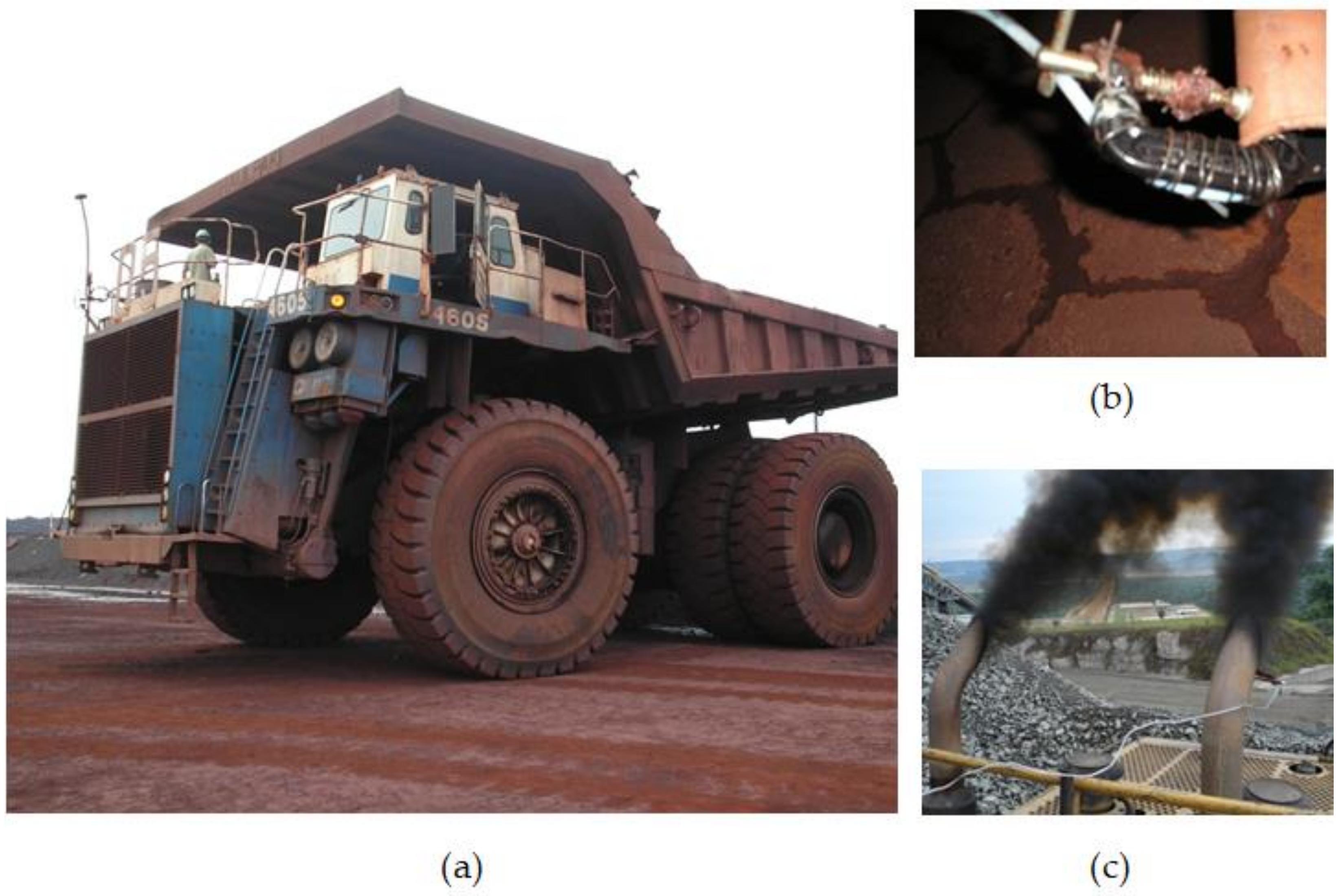
2.1. Emission Measurements

Figure 1a shows a photograph of a heavy-duty truck that is similar to the vehicles that were examined in this study. Its tires are 3.6 m in diameter, and it can carry 220 tons of ore. The employee standing in the truck gives a clear idea of its size.

A total of four trucks were investigated in this study, and they were designated #1 (Komatsu 830, Carajás), #2 (Komatsu 830, Carajás), #3 (Caterpillar 793C, Carajás), and #4 (Caterpillar 793C, Sossego). The Carajás mine is located in the state of Pará and the Sossego mine in the state of Minas Gerais, both in Brazil, and they belong to the Vale mining company.

Concentration measurements of the exhaust components were made by sampling the exhaust pipes of the trucks and determining the gas composition with a portable analyzer. The sampling was performed using a Teflon hose to avoid contamination or charring of the samples. This tubing contained a series of filters to remove large particles (greater than 100 µm) and moisture to prevent overloading of the analyzer’s filter system and to reduce the pressure drop in the instrument. The sampling tip was placed a few centimeters inside the exhaust pipe near the center of the circular section, as shown in Figure 1b. Figure 1c shows a case of particulate emissions from the exhaust pipe of a truck.

The device that was used to measure the gas composition was a portable multifunctional gas analyzer model Greenline 8000 from the company Eurotron, which performs continuous measurements. It determines the concentrations of oxygen (O₂), CO, and nitric oxide (NO) based on electrical signals that are emitted by electrochemical cells. It uses a nondispersive infrared (NDIR) system to analyze CO₂ and UHC. This instrument can also be used to measure the supply temperature and differential pressure, ambient temperature, and relative humidity. Its operating characteristics are summarized in

Table 1. Operational characteristics of the Greenline 8000 gas analyzer.

Parameter	Sensor Type	Limits	Resolution	Maximum Response Time (s)
O2	Electrochemical	0–25.0%	0.1%	20
CO	Electrochemical	0–20,000 ppm	1 ppm	40
CO2	NDIR	0–20.00%	0.01%	15
NO	Electrochemical	0–4000 ppm	1 ppm	40
CxHy	NDIR	0–50,000 ppm	1 ppm	15
Tamb	Pt100	−10–100 °C	0.1 °C
Tcomb gases	Thermocouple	0–1000 °C	0.1 °C
Pressure	Bridge	±150.00 hPa	0.01 hPa

. Concentrations of CO₂, O₂, CO, NO, and UHC were determined on a dry basis. The data were collected at 10-s intervals. Despite the amounts of particulates, the concentrations of CO and UHC were negligible in terms of mass balance. For the four trucks whose emissions were measured in this work,

Table 2. The number of points for which the ratio CO/CO₂ concentrations were below 3%, 2%, and 1%.

	Truck #1	Truck #2	Truck #3	Truck #4	Total	% of Total
# of points	457	347	417	635	1856	100.0%
Below 3%	456	347	412	622	1837	99.0%
Below 2%	452	346	397	618	1813	97.7%
Below 1%	431	329	305	509	1574	84.8%

presents the number of points for which the ratio CO/CO₂ concentrations were below 3%, 2%, and 1%, respectively. The average UHC volume concentration was 210 ppm for truck #1; this average was lower for the other trucks and was neglected in the carbon balance for all of them. The procedure considered the absence of sulfur in the diesel fuel.

The analyzer did not possess the capability of determining gases that were derived from sulfur. Some small amounts of the compound (<0.2%) could be expected. Sulfur could be expected to react completely to SO₂ and be accounted for in the procedure.

The mean volume concentrations of CO and NO were 650 and 280 ppm, respectively, for Truck #1. Although these concentrations are negligible, they were used to correct for the concentrations of CO₂ and O₂, as described in the following section.

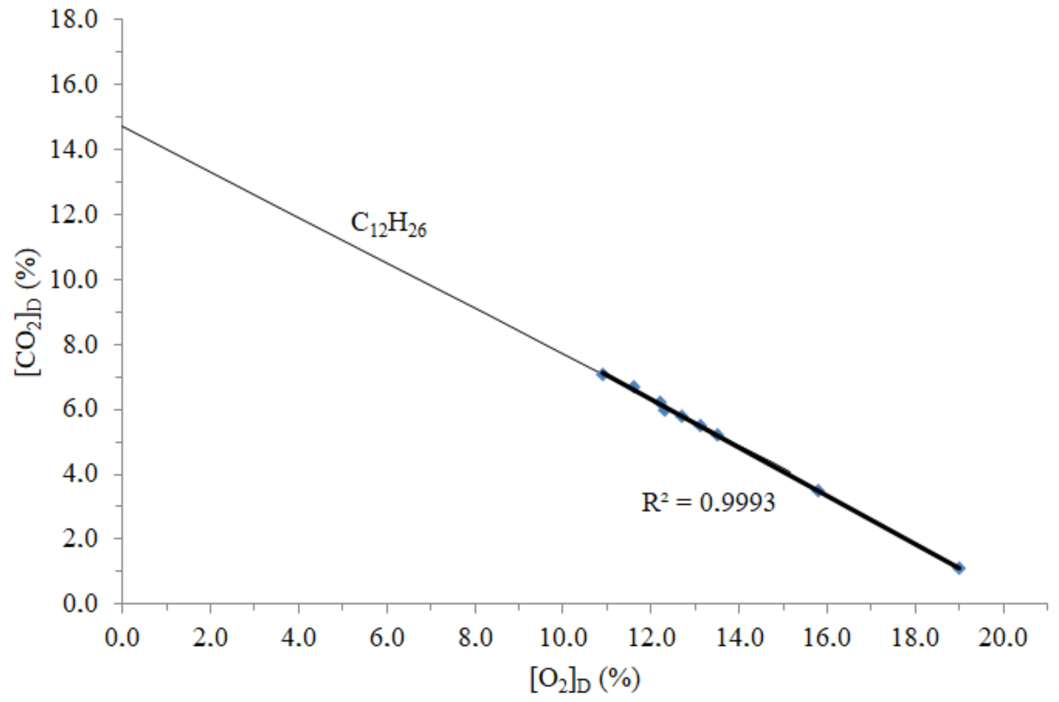
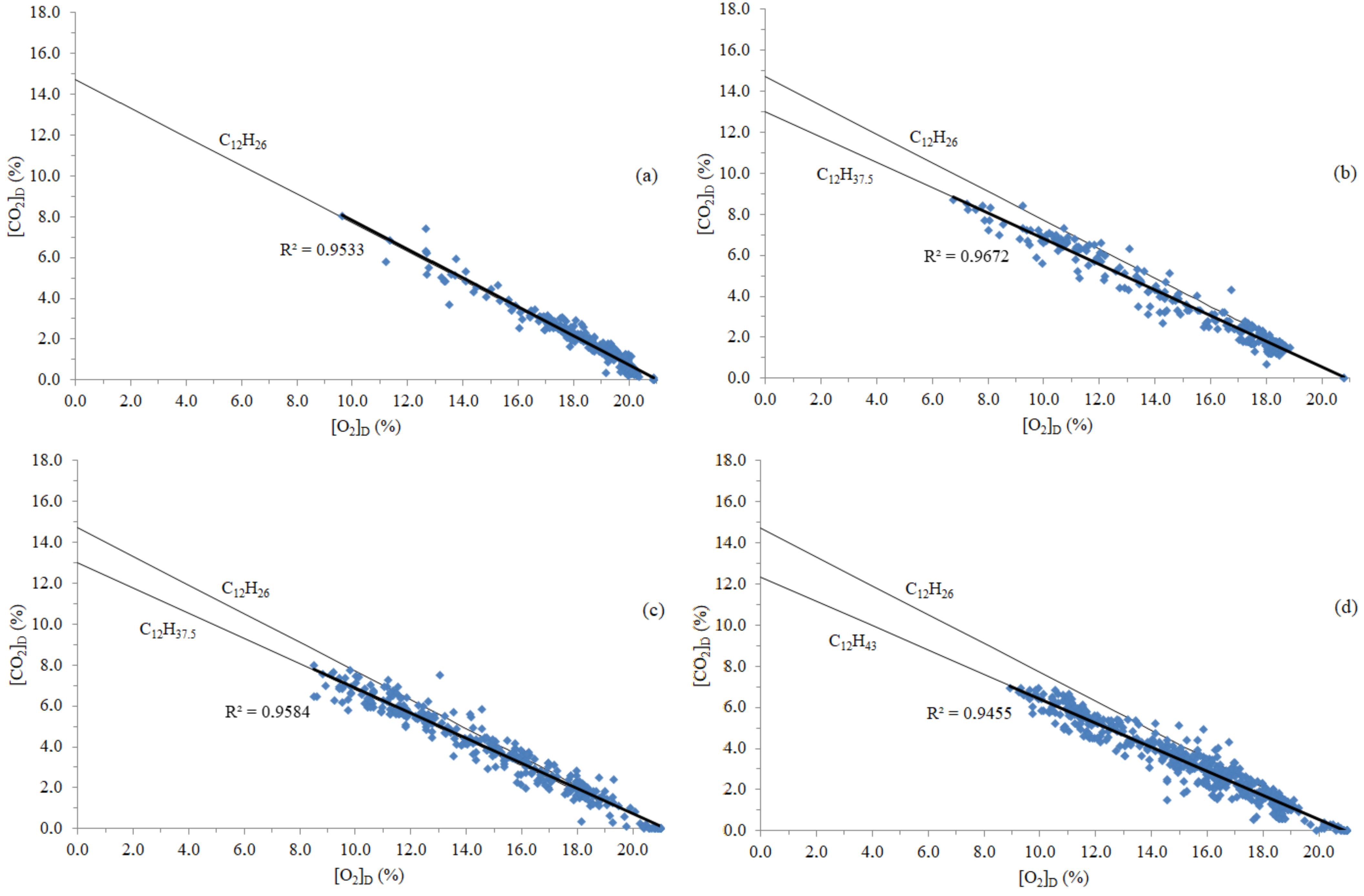
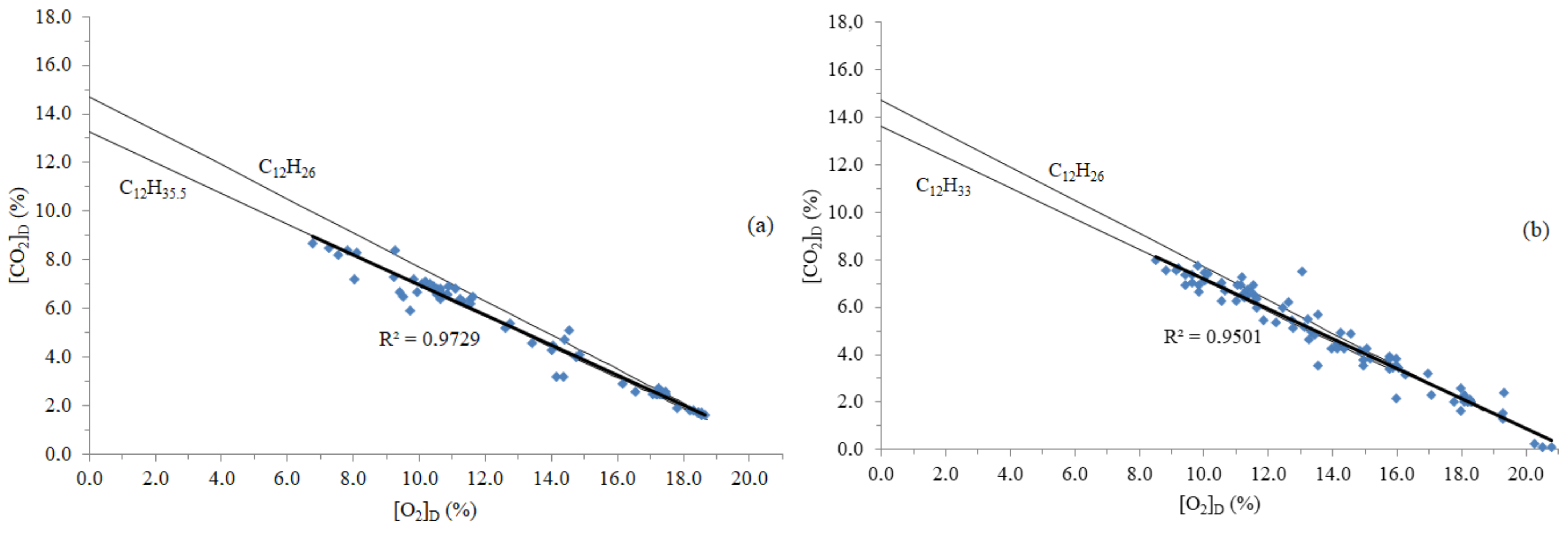
2.2. Diesel Formulation

No data were available on the formulation of the diesel fuel that was used in the heavy-duty engines. In addition, it was not possible to determine the exact composition of the diesel fuel that was used in the field. The concentrations of the exhaust components, determined by the Vale [40] locomotive mechanical workshop in Vitória, in the Brazilian state of Espírito Santo, were used to evaluate the composition of the diesel fuel and, consequently, the carbon content and the CO₂ emission factor. The data are presented in

Table 3. Concentrations of locomotive flue gas components [40].

[CO2] (%)	[O2] (%)	[CO] (%)	[SO2] (ppm)	[NOx] (p.p.m)	[CO2]corr (%)	[O2]corr (%)
7.0	11.0	0.08	15.8	447	7.1	10.9
6.6	11.7	0.05	18.5	487	6.7	11.6
6.1	12.3	0.04	24.8	478	6.2	12.2
6.0	12.4	0.02	27.8	408	6.0	12.3
5.8	12.8	0.03	21.8	443	5.8	12.7
5.5	13.2	0.03	10.8	432	5.5	13.1
5.2	13.5	0.01	22.0	257	5.2	13.5
3.5	15.8	0.01	13.5	133	3.5	15.8
1.1	19.0	0.01	12.5	44	1.1	19.0

. Each data point is the average result of four measurements.

The CO₂ concentration was corrected with CO concentration by taking [CO₂]_corr = [CO₂] + [CO], and the O₂ concentration was corrected with CO and NO_x (assumed to be NO) concentrations by taking [O₂]_corr = [O₂] − [CO]/2 − 2[NO]/10,000. where [CO] and [NO] are in % and ppm, respectively. These corrections imply that complete combustion of CO and NO can be assumed.

Note that NO is present in hundredths of a ppm in the combustion products, while NO₂ is present in a tenths of a ppm [41]. Therefore, assuming that all NO_x is present as NO does not lead to significant differences.

If a generic formula C₁₂H_x is used for the diesel fuel, its stoichiometric combustion reaction takes the form shown in Equation (1).

$${\mathrm{C}}_{12}{\mathrm{H}}_{\mathrm{x}}+{\mathrm{yO}}_2+3.76{\mathrm{yN}}_2\to 12{\mathrm{CO}}_2+\frac{\mathrm{x}}{2}{\mathrm{H}}_2\mathrm{O}+3.76{\mathrm{yN}}_2.$$

(1)

where y is obtained by the oxygen balance, that is, y = 12 + x/4. Thus, the combustion reaction for a normalized generic excess of air, a, can be represented by Equation (2).

$$\begin{gathered} {\mathrm{C}}_{12}{\mathrm{H}}_{\mathrm{x}}+\mathsf{\alpha }\left(12+\frac{\mathrm{x}}{4}\right){\mathrm{O}}_2+3.76\mathsf{\alpha }\left(12+\frac{\mathrm{x}}{4}\right){\mathrm{N}}_2\hspace{1em}\hspace{1em}\hspace{1em}\hspace{1em}\hspace{1em}\hspace{1em}\hspace{1em}\hspace{1em}\hspace{1em}\hspace{1em}\hspace{1em}\hspace{1em}\hspace{1em} \\ \to 12{\mathrm{CO}}_2+\frac{\mathrm{x}}{2}{\mathrm{H}}_2\mathrm{O}+3.76\mathsf{\alpha }\left(12+\frac{\mathrm{x}}{4}\right){\mathrm{N}}_2+\left(\mathsf{\alpha }-1\right)\left(12+\frac{\mathrm{x}}{4}\right){\mathrm{O}}_2 \end{gathered}$$

(2)

Then, the theoretical percent concentrations of CO₂ and O₂, in dry basis, in the absence of CO, are shown in Equations (3) and (4).

It can be easily demonstrated that the [CO₂]_D vs. [O₂]_D line is also a straight line for any C_cH_hN_nS_sO_o type fuel if sulfur is considered to react to SO₂, the above corrections for CO and NO are applied, and combustion air is above stoichiometry.

$${[{\mathrm{CO}}_2]}_{\mathrm{D}}=\frac{12\mathrm{x}}{12+\left(4.76\mathsf{\alpha }-1\right)\left(12+\frac{\mathrm{x}}{4}\right)}100\%$$

(3)

$${[{\mathrm{O}}_2]}_{\mathrm{D}}=\frac{\left(\mathsf{\alpha }-1\right)\left(12+\frac{\mathrm{x}}{4}\right)}{12+\left(4.76\mathsf{\alpha }-1\right)\left(12+\frac{\mathrm{x}}{4}\right)}100\%$$

(4)

Isolating α from Equations (3) and (4), a descending straight-line relating [O₂]_D and [CO₂]_D is obtained:

$${[{\mathrm{O}}_2]}_{\mathrm{D}}=\frac{1200-\left(57.12+0.94\mathrm{x}\right){[{\mathrm{CO}}_2]}_{\mathrm{D}}}{57.12}$$

(5)

The value of x in Equations (3) and (4) was adjusted to fit the data of Table 3. The result is x = 26, as shown in Figure 2. The stoichiometric combustion reaction for a fuel with a molecule C₁₂H₂₆ is given in Equation (6).

$${\mathrm{C}}_{12}{\mathrm{H}}_{26}+18.5{\mathrm{O}}_2+69.56{\mathrm{N}}_2\to 12{\mathrm{CO}}_2+13{\mathrm{H}}_2\mathrm{O}+69.56{\mathrm{N}}_2$$

(6)

and its CO₂ emission factor, for complete combustion, in terms of kg/kg is obtained as shown in Equation (7).

$${\mathrm{EF}}_{\mathrm{diesel}}=\frac{12\times 44}{12\times 12+26}=3.106\frac{{\mathrm{kg} \mathrm{CO}}_2}{\mathrm{kg} \mathrm{diesel}}$$

(7)

The concentrations of gases that are produced by the combustion of a diesel fuel that is obtained from a gas station in the city of Cachoeira Paulista, São Paulo State, Brazil, were measured [42]. Using the same procedure as here, the formula C₁₂H_21.15 was determined. The corresponding emission factor for complete combustion was 2.9% higher, with a value of EFdiesel = 3.197 kg − CO₂/kg-diesel.

In Brazil, the density of diesel fuel ranges from 0.82 kg/L (light diesel) to 0.88 kg/L (heavy diesel) [43]. This gives an average density of 0.85 kg/L, and using the EF that is given in [42], the emission factor in kg/L is 2.717 kgCO₂/L of fuel. This value, with a deviation of 0.48%, compares very favorably with the value of 2.730 kgCO₂/L of fuel that is given by ECC Canada [44].

The combustion of diesel fuel in heavy machinery in mining operations produces a significant amount of particulate matter [see Figure 1b] which must be considered when calculating the actual emission factor for the activity. The particulate matter is not directly quantifiable but can be accounted for by measuring the concentrations of product gases that are generated by the equipment.

2.3. Fuel Losses to Particles

The engine does not operate under the same conditions during the different maneuvers that are required during the tasks that the truck has to perform. In addition, trucks have different ages and maintenance schedules that can affect their performance.

The losses can be estimated if it is assumed that the engine only partially consumes the heavy diesel compounds and forms the dark smoke, which consists of a large amount of carbon. Consider a diesel fuel with the general formula C₁₂Ha, which releases particulates during combustion. If we consider the effective combustion of a lighter diesel fuel (C₁₂H_b) as a result of the emission of particles, the balance of hydrogen atoms leads to:

$${\mathrm{C}}_{12}{\mathrm{H}}_{\mathrm{a}}=\frac{\mathrm{a}}{\mathrm{b}}\left({\mathrm{C}}_{12}{\mathrm{H}}_{\mathrm{b}}+\mathrm{yC}\right)$$

(8)

with b > a, being y the number of moles of carbon per mole of C₁₂H_b. For carbon, the balance leads to:

$$\mathrm{y}=12\left(\frac{\mathrm{b}}{\mathrm{a}}-1\right)$$

(9)

The carbon loss is, then:

$$\mathrm{C}\left(\%\right)=\frac{144\left(1-\frac{\mathrm{a}}{\mathrm{b}}\right)}{144+\mathrm{a}}100\%$$

(10)

It is clear that the carbon loss given by Equation (10) cannot be determined by the ratio a/b alone, i.e., the value of “a” is necessary for the analysis. This value was assumed to be 26, as determined with the data from the laboratory of the locomotives.

Assuming a diesel fuel with a calorific value of 43 MJ/kg [17] and that the calorific value of carbon is 32.76 MJ/kg, the percentage of the fuel’s calorific value that is lost as soot particles is:

$$\mathrm{Energy} \mathrm{loss} \left(\%\right)=0.762\frac{144\left(1-\frac{\mathrm{a}}{\mathrm{b}}\right)}{144+\mathrm{a}}100\%$$

(11)

It should be mentioned that this method does not determine the overall energy efficiency of the device. This depends on many other parameters than only carbon loss as particles. Moreover, it was assumed that the carbon loss occurs only in the form of carbon particles, which is confirmed by the conditions that were observed during the field measurements.

2.4. Fuel Losses to Carbon Monoxide and Unburned Hydrocarbons

Other losses may be considered, e.g., to CO and UHC if they occur in non-negligible concentrations. For UHC, the assumption can be made that it is CH₄, since this is the main compound of the UHC mixture.

The following formula can be established for a general chemical reaction between fuel and air:

Fuel + Air →
x₁ CO + x₂ CO₂ + x₃ SO₂ + x₄ N₂ + x₅ NO + x₆ C_mH_n + x₇ O₂ + x₈ H₂O + Particles.

(12)

Instruments that measure the concentrations of gas constituents usually report the values as a dry basis. Water interferes with most detection systems of analytical instruments. On a dry basis (subscript D) is the molar fraction of each gaseous combustion product:

$${[\mathrm{X}]}_{\mathrm{i},\mathrm{D}}=\frac{{\mathrm{x}}_{\mathrm{i}}}{{\displaystyle \sum _1^7{\mathrm{x}}_{\mathrm{i}}}}$$

(13)

These molar fractions are important when determining the mass flow rate of carbon in each of the combustion products, as shown in the following. Particles do not interfere with concentrations of gas components.

It is necessary to determine the concentrations of CO₂, CO, C_mH_n, and particles in the combustion gases, and the carbon content of such particles.

Applying a mass balance, the mass flow rate of carbon that is emitted as CO₂, ṁ_C,CO2, through the several stacks and as fugitive emissions, is:

$${\dot{\mathrm{m}}}_{\mathrm{C},\mathrm{C}{\mathrm{O}}_2}={\dot{\mathrm{m}}}_{\mathrm{C},\mathrm{fuel}}-{\dot{\mathrm{m}}}_{\mathrm{C},\mathrm{CO}}-{\dot{\mathrm{m}}}_{\mathrm{C},\mathrm{part}}-{\dot{\mathrm{m}}}_{\mathrm{C},{\mathrm{C}}_{\mathrm{m}}{\mathrm{H}}_{\mathrm{n}}},$$

(14)

where ṁ_C,fuel is the mass flow rate of carbon that enters the truck with the diesel fuel, ṁ_C,CO is the mass flow rate of carbon that is emitted as CO, ṁ_C,part is the mass flow rate of carbon that is emitted in the particulate material, and ṁ_C,CmHn is the mass flow rate of carbon that is emitted as unburned gaseous hydrocarbons C_mH_n.

The mass flow rate of carbon in the inlet of the equipment is ṁ_C,fuel = Y_C,fuelṁ_fuel, where Y_C,fuel is the total carbon content in ṁ_fuel.

The mass flow ratios of carbon that are emitted CO₂, to CO and C_mH_n species, are related by the concentrations of such gases, in a dry basis, in the combustion products, as shown in

$${\dot{\mathrm{m}}}_{\mathrm{C},{\mathrm{x}}_{\mathrm{i}}}=\mathrm{m}\frac{{\mathrm{x}}_{\mathrm{i}}}{{\mathrm{x}}_1}{\dot{\mathrm{m}}}_{\mathrm{C},\mathrm{C}{\mathrm{O}}_2}=\mathrm{m}\frac{{[\mathrm{X}]}_{\mathrm{i},\mathrm{D}}}{{[\mathrm{C}{\mathrm{O}}_2]}_{\mathrm{D}}}{\dot{\mathrm{m}}}_{\mathrm{C},\mathrm{C}{\mathrm{O}}_2}$$

(15)

where m = 1 for CO. Thus, the relationship between the mass flow rates of carbon as CO and as CO₂ is [CO]_D/[CO₂]_D. For CH₄, the relationship is [CH₄]_D/[CO₂]_D. These represent the losses to CO and CH₄, respectively, on the assumption that their volume concentrations can be measured.

In the case of the particulate material emission, to obtain ṁ_C,part as function of ṁ_C,CO2, it is necessary to determine the concentration of particulate material that is emitted by the equipment through its several exhaust tubes and the carbon content of each of the respective samples. This requires adequate equipment and careful procedures, as described in the EPA Method number 5, and is impractical with heavy trucks performing different maneuvers. The term ṁ_C,part is obtained from the procedure outlined in the previous subsection.

Therefore, with the previous considerations, Equation (14) leads to the following for the mass flow rate of emitted CO₂:

$${\dot{\mathrm{m}}}_{\mathrm{C}{\mathrm{O}}_2}=\frac{44}{12}\frac{{\mathrm{Y}}_{\mathrm{C},\mathrm{fuel}}{\dot{\mathrm{m}}}_{\mathrm{fuel}}}{1+\frac{{[\mathrm{CO}]}_{\mathrm{D}}}{{[\mathrm{C}{\mathrm{O}}_2]}_{\mathrm{D}}}+\frac{\mathrm{m}{[{\mathrm{C}}_{\mathrm{m}}{\mathrm{H}}_{\mathrm{n}}]}_{\mathrm{D}}}{{[\mathrm{C}{\mathrm{O}}_2]}_{\mathrm{D}}}+\frac{{\dot{\mathrm{m}}}_{\mathrm{part}}}{{\dot{\mathrm{m}}}_{\mathrm{C}{\mathrm{O}}_2}}}$$

(16)

where the factor 44/12 corresponds to the relative mass of carbon dioxide to the mass of carbon in a carbon dioxide molecule.

3. Results and Discussion

3.1. Time Concentrations, Carbon and Energy Losses, and Emission Factors

Figure 3 shows the time variation of the O₂ and CO₂ concentration for all the trucks. It includes operation in idle (during loading, unloading, and waiting in line), and when in movement (with and without load).

As expected, the O₂ and CO₂ concentration data are consistent with each other, that is, a decrease in the O₂ concentration goes together with an increase in the CO₂ concentration, and vice versa. While Trucks #1, #2, and #3 performed operations that did not repeat (with #1 in idle for a long period), Truck #4 performed four similar tasks, as shown if Figure 3d by the peaks. The correlations between the measured instantaneous O₂ and CO₂ concentrations will be examined below.

The CO₂ concentration was plotted as function of the O₂ concentration for each data point. The value of x was allowed to fluctuate and the dependence between the CO₂ and O₂ concentrations, given by Equations (3) and (4), was fit to the experimental values. Figure 4 shows the results of such procedure for all trucks. The values of x that give the best match against the experimental data, whose linear fit was plotted in a bold straight line, are shown in the figure. They were x = 26 for #1, x = 37.5 for #2, x = 37.5 for #3, and x = 43 for #4. The R² coefficient was higher than 0.94 in all cases.

It was observed that Truck #1 produced concentration results that fitted the diesel formulation, while the others presented carbon losses and, consequently, lower average CO₂ emission factors.

Table 4. Average carbon and energy losses.

	Carbon Loss	Energy Loss
Truck #1	0.0%	0.0%
Truck #2	26.0%	19.8%
Truck #3	26.0%	19.8%
Truck #4	33.5%	25.5%

presents the average carbon and energy losses for all the trucks. The results for Trucks #2 to #4 are a consequence of the very sooty emissions, such as that shown in Figure 1c.

Table 5 presents the average emission factors for all the trucks. The reference value is given by ECC Canada [44], and the default value is given by IPCC [17]. It was observed that each of the trucks burnt diesel fuel with different sets of maneuvers, in addition to possible differences between the trucks themselves and, therefore, different emission factors were obtained. The average EF of Truck #4 was 64.8% of the IPCC value, which led to a CO₂ emission 33.5% lower than that which was obtained by computing it with the default EF for the diesel fuel considered here. The emissions factors that were obtained by Li et al. [35] are presented in the same table.

A lower emission factor does not mean that the corresponding unit will emit less CO₂; in fact, it will require larger quantities of diesel fuel to meet its energy requirements. Suppose that a truck is very well maintained and regulated, so that it emits a negligible amount of particles, being m the mass of fuel that is consumed to perform a determined task. Now, suppose a truck in a second situation, working with the characteristics of Truck #4, performing the same task, which can be estimated to require the same amount of energy. Taking the energy loss given in Table 4 for Truck #4 (25.5%), the mass of fuel that is required to perform the same task will be 1/0.745 ·m = 1.342 m, and this is considering that the calorific value of the fuel does not decrease under the second situation.

Applying the factor 1.342 the emission factor of Truck #4 becomes 2.771. Comparing our results with those that were obtained by Li et al. [35], it is noticed that only the Truck#1 presents an emissions factor similar to that by Li et al. [35]. On the other hand, the Trucks #2, #3, and #4 presented lower emission factors. This is related to the fact that during the operation of Trucks #2, #3, and #4, the particulate matter emissions were higher than those for Truck #1. Therefore, the method that is presented in this article allows the identification of significant losses in the form of particulate matter, which manifest when the emission factor is lower than that which is determined by Equation (7).

It can be argued that the average emission factor that was calculated by the procedure developed here does not represent the real CO₂ emission of the unit, since much higher amounts of fuel are burned during movement, especially during acceleration, in comparison with operation in idle. The effect of operation under lower O₂ and higher CO₂ concentrations, characteristics of movement, was examined. The objective of doing this is to analyze the operation intervals for which the O₂ and CO₂ concentrations were lower and higher, respectively. These intervals represent a regime of operation of the engines. Other periods were not selected because they did not comply with this condition.

Table 5. The average emission factors.

Source	Emission Factor (kg CO2/kg Diesel)	% Default Value (IPCC [17])
Laboratory [42]	3.197	100.3%
Laboratory [40]	3.106	97.5%
Truck #1	3.106	97.5%
Truck #2	2.298	72.1%
Truck #3	2.298	72.1%
Truck #4	2.065	64.8%
Li et al. (Truck) [35]	3.157	99.1%
Li et al. (Truck) [35]	3.183	99.9%
ECC Canada [44]	3.212 a	100.8%
IPCC [17]	3.186 b	100.0%

^a For an average density of 0.85 kg/L; ^b 74100 kg CO₂/TJ; Net Calorific Value = 43.0 TJ/Gg.

Table 5. The average emission factors.

Source	Emission Factor (kg CO2/kg Diesel)	% Default Value (IPCC [17])
Laboratory [42]	3.197	100.3%
Laboratory [40]	3.106	97.5%
Truck #1	3.106	97.5%
Truck #2	2.298	72.1%
Truck #3	2.298	72.1%
Truck #4	2.065	64.8%
Li et al. (Truck) [35]	3.157	99.1%
Li et al. (Truck) [35]	3.183	99.9%
ECC Canada [44]	3.212 a	100.8%
IPCC [17]	3.186 b	100.0%

^a For an average density of 0.85 kg/L; ^b 74100 kg CO₂/TJ; Net Calorific Value = 43.0 TJ/Gg.

First, some portions of Figure 3b,c were deliberately cut to observe changes in the emission factor. These cuts, made to take into account operation at lower excess of air, were the following:

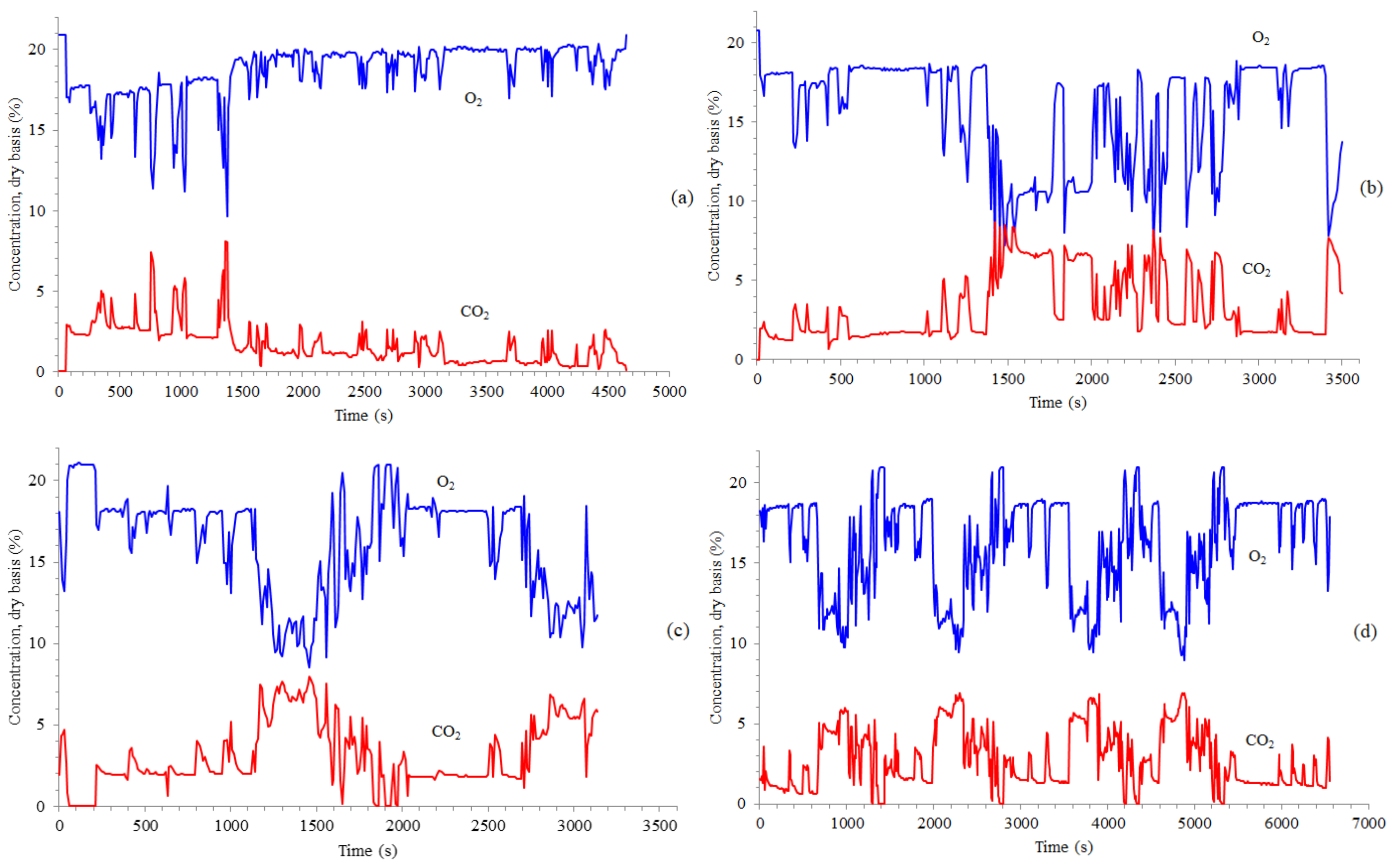
• Truck #2: the original 350 points, corresponding to 0–3490 s, were substituted by 86 points, corresponding to 1260–2110 s;
• Truck #3: the original 460 points, corresponding to 0–4590 s, were substituted by 85 points, corresponding to 990–1830 s.

The results of such cuts are presented in Figure 5. It is noted that the R² coefficient remains practically unchanged.

The main results that were obtained from Figure 5 indicate changes between the overall and selected periods of operation, according to:

• Truck #2: average EF of 2.298 kg CO₂/kg diesel becomes 2.401 kg CO₂/kg diesel (4.5% change, 75.4% of IPCC default value); average carbon loss of 26.0% becomes 22.7% (3.3% difference);
• Truck #3: average EF of 2.298 kg CO₂/kg diesel becomes 2.547 kg CO₂/kg diesel (10.8% change, 79.9% of IPCC default value); average carbon loss of 26.0% becomes 18.0% (8.0% difference).

Next, some portions of Figure 3d were also deliberately cut to observe changes in the emission factor, but the approach was somewhat different:

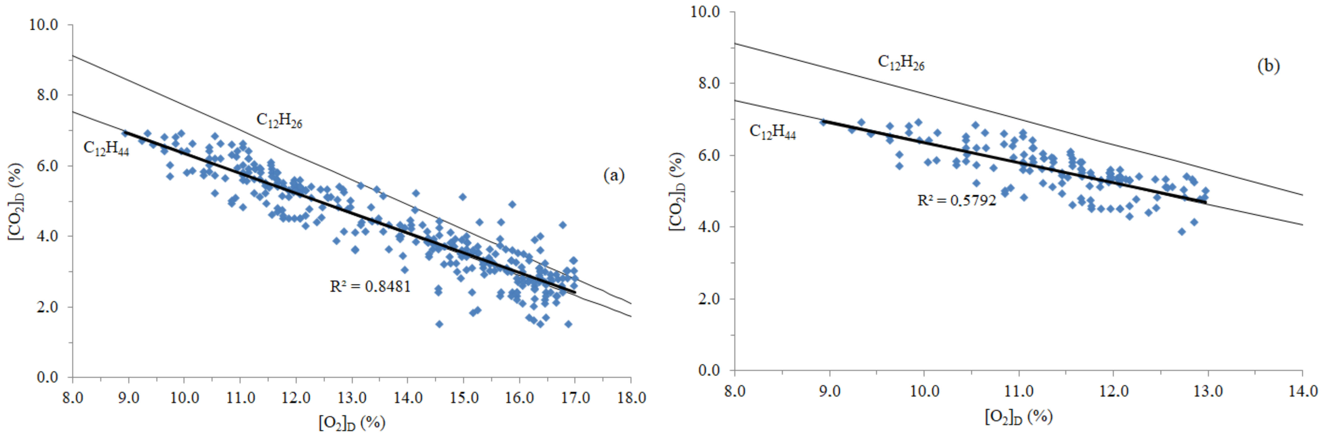
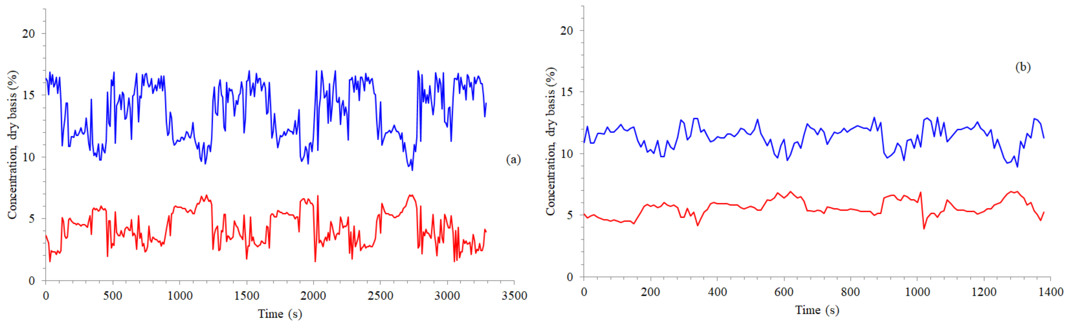
• Truck #4: the original 655 points were substituted by 329 points, corresponding to operation under [O₂]_D < 17%;
• Truck #4: the original 655 points were substituted by 138 points, corresponding to operation under [O₂]_D < 13%.

The time variation of O₂ and CO₂ concentrations with time (in a continuous basis), for the above-described situations, is presented in Figure 6. As the O₂ concentration is limited to a certain value, the graph represents operation at richer conditions and consistent with higher mass flow rates of fuel. Figure 7 presents the CO₂ concentration as function of O₂ concentration, also for the above-described situations. A steep reduction of the R² coefficient is observed; however, the emission factor and the carbon loss remained practically the same as those that were calculated for overall average conditions.

Figure 6 and Figure 7 are examples of how sampling can be divided into specific maneuver periods or conditions so that they can be assessed individually. The difference between the squared correlation coefficients happens because for the low air excess regime, there are fewer data than for high air excess.

3.2. Error Estimates

The resolutions of the O₂ and CO₂ sensors were 0.1% and 0.01%, respectively, as shown in Table 1. The errors were estimated by carrying out the same procedure that was used to obtain Figure 4, but adding and subtracting 0.1% and 0.01% to the measured concentrations of O₂ and CO₂, respectively.

Table 6. The results for the error in relation to the calculated emission factor.

Truck	Action	Fuel Formula	Emission Factor Error a
#1	+ +	C12H24.3	5.9%
	+ −	C12H24.3	5.9%
	− −	C12H26.1	−0.3%
	− +	C12H26.1	−0.3%
#2	+ +	C12H36.4	2.4%
	+ −	C12H36.4	2.4%
	− −	C12H37.8	−0.6%
	− +	C12H37.5	0.0%
#3	+ +	C12H35.9	3.5%
	+ −	C12H36.0	3.3%
	− −	C12H37.6	−0.2%
	− +	C12H37.6	−0.2%
#4	+ +	C12H43.2	−0.4%
	+ −	C12H43.1	−0.2%
	− −	C12H43	0.0%
	− +	C12H43.1	−0.2%

^a In relation to the value that was calculated in the respective graph.

presents the results. In the column named “Action”, + + represents +0.1% and +0.01%, and so on. It is observed that, under the conditions of the unpredictable maneuvers that were performed by the trucks during the data collection of this work, the maximum estimated error was 5.9%, which occurred for Truck #1.

4. Conclusions

A simple and novel method for determining CO₂ emission rates and carbon losses for heavy-duty vehicles was developed.

A series of four off-road heavy-duty trucks used to transport iron ore were analyzed for their CO₂ emission rates and carbon losses. The importance of gas concentration measurements in inferring instantaneous fuel composition, which can vary depending on the maneuver being performed and truck parameters such as age, maintenance records, type, etc., was demonstrated.

It has been shown that each of the four off-road trucks consumes diesel fuel with different efficiency and, therefore, each of them has a different average emission factor. The results for Truck #4 show that the average CO₂ emission factors can be as low as 64.8% of the IPCC default value for diesel fuel. On the other hand, even for Truck #4, losses can reach 33.5% in terms of carbon and 25.5% in terms of energy.

A limitation of the present study was the fact that it used the diesel oil formulation that was obtained in the laboratory for locomotives. The fuel had to be analyzed in the mining area before being used in the trucks, which was not possible. Another limitation was the difficulty in providing a valid error analysis for all situations in an unpredictable set of general truck characteristics and maneuvers. However, these do not invalidate the method that was developed here.

A similar line of thought has been applied in the past by two of the authors to: (a) detect and quantify leakage from coke ovens to combustion chambers in a conventional coke plant, and (b) detect and estimate scale formation in slab reheating furnaces. This work is available in the form of consulting reports. In the first case, carbon particles infiltrated the combustion chamber where coke oven gas (COG) was burned; the effective fuel was replaced by a mixture of COG and carbon particles. In the second case, oxygen was removed from the combustion products of natural gas by scale formation; the effective fuel was replaced by a mixture of natural gas and iron.

In future work, the authors intend to test the method with a portable emissions measurement system in order to develop a tool that be used to estimate the emissions factors in real time, during the normal operation of a heavy-duty vehicle.

The authors believe that the procedure that was outlined in this article, if carried out with proper error analysis, can be useful in problems involving energy losses in industrial combustion processes.

References

1. Barrett, S. Political economy of the kyoto protocol. Clim. Chang. 2017, 14, 465–484. [Google Scholar] [CrossRef]
2. Springer, U. The market for tradable GHG permits under the Kyoto Protocol: A survey of model studies. Energy Econ. 2003, 25, 527–551. [Google Scholar] [CrossRef]
3. Johnson, E.; Heinen, R. Carbon trading: Time for industry involvement. Environ. Int. 2004, 30, 279–288. [Google Scholar] [CrossRef] [PubMed]
4. Karpf, A.; Mandel, A.; Battiston, S. Price and network dynamics in the European carbon market. J. Econ. Behav. Organ. 2018, 153, 103–122. [Google Scholar] [CrossRef] [Green Version]
5. Watson, F. Global Carbon Market Grows 20% to $272 Billion in 2020: Refinitiv; S&P Glob Patts: London, UK, 2021. [Google Scholar]
6. Aldhous, P. China’s Burning Ambition. Nature 2005, 435, 1152–1156. [Google Scholar] [CrossRef] [PubMed]
7. Hopke, P.K. Contemporary threats and air pollution. Atmos. Environ. 2009, 43, 87–93. [Google Scholar] [CrossRef]
8. Wang, R.; Liu, W.; Xiao, L.; Liu, J.; Kao, W. Path towards achieving of China’s 2020 carbon emission reduction target-A discussion of low-carbon energy policies at province level. Energy Policy 2011, 39, 2740–2747. [Google Scholar] [CrossRef]
9. Auffhammer, M.; Carson, R.T. Forecasting the path of China’s CO2 emissions using province-level information. J. Environ. Econ. Manag. 2008, 55, 229–247. [Google Scholar] [CrossRef] [Green Version]
10. Ouyang, X.; Fang, X.; Cao, Y.; Sun, C. Factors behind CO2 emission reduction in Chinese heavy industries: Do environmental regulations matter? Energy Policy 2020, 145, 111765. [Google Scholar] [CrossRef]
11. Gerlagh, R.; Lise, W. Carbon taxes: A drop in the ocean, or a drop that erodes the stone? The effect of carbon taxes on technological change. Ecol. Econ. 2005, 54, 241–260. [Google Scholar] [CrossRef]
12. Michaelowa, A.; Stronzik, M.; Eckermann, F.; Hunt, A. Transaction costs of the kyoto mechanisms. Clim. Policy 2003, 3, 261–278. [Google Scholar] [CrossRef] [Green Version]
13. Nagase, K. “Carbon-Money Exchange” to contain global warming and deforestation. Energy Policy 2005, 33, 1233–1238. [Google Scholar] [CrossRef]
14. ISO 14064-1:2018; Greenhouse Gases—Part 1: Specification with Guidance at the Organization Level for Quantification and Reporting of Greenhouse Gas Emissions and Removals. ISO: Geneva, Switzerland, 2019.
15. Friedl, B.; Getzner, M. Determinants of CO2 emissions in a small open economy. Ecol. Econ. 2003, 45, 133–148. [Google Scholar] [CrossRef]
16. Katta, A.K.; Davis, M.; Kumar, A. Assessment of greenhouse gas mitigation options for the iron, gold, and potash mining sectors. J. Clean. Prod. 2020, 245, 118718. [Google Scholar] [CrossRef]
17. Inventories TF on NGG. 2019 Refinement to the 2006 IPCC Guidelines for National Greenhouse Gas Inventories—General Guidance and Reporting; IPCC, United Nations: Geneva, Switzerland, 2019; Volume 1. [Google Scholar]
18. Benajes, J.; García, A.; Monsalve-Serrano, J.; Martínez-Boggio, S. Potential of using OMEx as substitute of diesel in the dual-fuel combustion mode to reduce the global CO2 emissions. Transp. Eng. 2020, 1, 100001. [Google Scholar] [CrossRef]
19. Song, H.; Ou, X.; Yuan, J.; Yu, M.; Wang, C. Energy consumption and greenhouse gas emissions of diesel/LNG heavy-duty vehicle fleets in China based on a bottom-up model analysis. Energy 2017, 140, 966–978. [Google Scholar] [CrossRef]
20. Lao, J.; Song, H.; Wang, C.; Zhou, Y.; Wang, J. Beijing- Reducing atmospheric pollutant and greenhouse gas emissions of heavy duty trucks by substituting diesel with hydrogen in Tianjin-Hebei-Shandong region, China. Int. J. Hydrogen Energy 2021, 46, 18137–18152. [Google Scholar] [CrossRef]
21. Xing, Y.; Song, H.; Yu, M.; Wang, C.; Zhou, Y.; Liu, G.; Du, L. The Characteristics of Greenhouse Gas Emissions from Heavy-Duty Trucks in the Beijing-Tianjin-Hebei (BTH) Region in China. Atmosphere 2016, 7, 121. [Google Scholar] [CrossRef] [Green Version]
22. González, R.M.; Marrero, G.; Rodriguez-López, J.; Marrero, A.S. Analyzing CO2 emissions from passenger cars in Europe: A dynamic panel data approach. Energy Policy 2019, 129, 1271–1281. [Google Scholar] [CrossRef]
23. Li, X.; Yu, B. Peaking CO2 emissions for China’s urban passenger transport sector. Energy Policy 2019, 133, 110913. [Google Scholar] [CrossRef]
24. Breed, A.; Speth, D.; Plötz, P. CO2 fleet regulation and the future market diffusion of zero-emission trucks in Europe. Energy Policy 2021, 159, 112640. [Google Scholar] [CrossRef]
25. Anderhofstadt, B.; Spinler, S. Preferences for autonomous and alternative fuel-powered heavy-duty trucks in Germany. Transp. Res. Part D Transp. Environ. 2020, 79, 102232. [Google Scholar] [CrossRef]
26. Quiros, D.; Smith, J.; Thiruvengadam, A.; Huai, T.; Hu, S. Greenhouse gas emissions from heavy-duty natural gas, hybrid, and conventional diesel on-road trucks during freight transport. Atmos. Environ. 2017, 168, 36–45. [Google Scholar] [CrossRef]
27. Tietge, U.; Mock, P.; Franco, V.; Zacharof, N. From laboratory to road: Modeling the divergence between official and real-world fuel consumption and CO2 emission values in the German passenger car market for the years 2001–2014. Energy Policy 2017, 103, 212–232. [Google Scholar] [CrossRef]
28. Brizuela, E. A novel presentation of Ostwald´s combustion. Ind. Comb. J. Int. Flame Res. Found. 2015. Available online: https://ifrf.net/research/archive/a-novel-presentation-of-ostwalds-combustion/ (accessed on 15 January 2022).
29. Clairotte, M.; Suarez-Bertoa, R.; Zardini, A.; Giechaskiel, B.; Pavlovic, J.; Valverde, V.; Ciuffo, B.; Astorga, C. Exhaust emissions factors of greenhouse gases (GHGs) from European road vehicles. Environ. Sci. Eur. 2020, 32, 125–145. [Google Scholar] [CrossRef]
30. Wang, H.; Wu, Y.; Zhang, K.; Zhang, S.; Baldauf, R.; Snow, R.; Deshmukh, P.; Zheng, X.; He, L.; Hao, J. Evaluating mobile monitoring of on-road emission factors by comparing concurrent PEMS measurements. Sci. Total Environ. 2020, 736, 139507–139517 . [Google Scholar] [CrossRef]
31. Liu, Y.; Tan, J. Green traffic-oriented heavy-duty vehicle emissions characteristics of China VI based on portable emission measurement systems. IEEE Access 2020, 8, 106639–106647 . [Google Scholar] [CrossRef]
32. He, L.; Zhang, S.; Hu, J.; Li, Z.; Zheng, X.; Cao, Y.; Xu, G.; Yan, M.; Wu, Y. On-road emission measurements of reactive nitrogen compounds from heavy-duty diesel trucks in China. Environ. Pollut. 2020, 262, 114280–114290. [Google Scholar] [CrossRef]
33. Anable, J.; Brand, C.; Tran, M.; Eyre, N. Modelling transport energy demand: A socio-technical approach. Energy Policy 2012, 41, 125–138. [Google Scholar] [CrossRef] [Green Version]
34. Linton, C.; Grant-Muller, S.; Gale, W. Approaches and techniques for modelling CO2 emissions from road transport. Transp. Rev. 2015, 35, 533–553. [Google Scholar] [CrossRef]
35. Li, X.; Ai, Y.; Ge, Y.; Qi, J.; Feng, Q.; Hu, J.; Porter, W.; Miao, Y.; Mao, H.; Jin, T. Integrated effects of SCR, velocity, and air-fuel ratio on gaseous pollutants and CO2 emissions from China V and VI heavy–duty diesel vehicles. Sci. Total Environ. 2022, 811, 152311–152319. [Google Scholar] [CrossRef]
36. Nguyen, X.; Hoang, A.; Olçer, A.; Huynh, T. Record decline in global CO2 emissions prompted by COVID-19 pandemic and its implications on future climate changes policies. Energy Sources Part A 2021. [Google Scholar] [CrossRef]
37. Hoang, T.; Nizetic, S.; Olcer, A.; Ong, H.; Chen, W.; Chong, C.; Thomas, S.; Bandh, S.; Nguyen, X. Impacts of COVID-19 on the global energy system and shift progress to renewable energy: Opportunities, challenges and policy implications. Energy Policy 2021, 154, 112322. [Google Scholar] [CrossRef]
38. Nguyen, H.; Hoang, A.; Nizetic, S.; Nguyen, X.; Le, A.; Luong, C.; Chi, V.; Pham, V. The electric propulsion system as a green solution for management strategy of CO2 emissions in ocean shipping: A comprehensive review. Int. Trans. Electr. Energy Syst. 2021, 31, e12580. [Google Scholar] [CrossRef]
39. Hoang, A.; Pham, V.; Nguyen, X. Integrating renewable sources into energy system for smart city as a sagacious strategy towards clean and sustainable process. J. Clean. Prod. 2021, 305, 127161. [Google Scholar] [CrossRef]
40. Portela, P.; Coelho, F.; Vale Mining Company. Personal Communication, 2007.
41. Borman, G.; Ragland, K. Combustion Engineering; McGraw-Hill: New York, NY, USA, 1998; pp. 125–126. [Google Scholar]
42. Paz, E. Substitution of Diesel Fuel by Ethyl Alcohol in Industrial Burners. Ph.D. Thesis, Universidade Estadual Paulista Julio de Mesquita Filho, Guartinguetá, Brazil, 2007. (In Portuguese). [Google Scholar]
43. Garcia, R. Fuels and Industrial Combustion. Interciência: Rio de Janeiro, Brazil, 2002. (In Portuguese) [Google Scholar]
44. ECC Canada. Environment and Climate Change Canada. Greenhouse Gas Emissions—Canadian Environmental Sustainability Indicators; ECC Canada: Gatineau, QC, Canada, 2020; Volume 4. [Google Scholar]
Figure 1. Photographs of: (a) an off-road truck for transporting iron ore, (b) the gas sampling nozzle, (c) a set of two exhaust pipes. Source: the authors.
Energies 15 02659 g001
Figure 2. The CO2 concentration as a function of O2 concentration, both on a dry basis, for diesel fuel combustion in locomotives. Experimental data source: [40].
Energies 15 02659 g002
Figure 3. The O2 and CO2 concentrations as functions of time for all trucks: #1 (a), #2 (b), #3 (c), and #4 (d).
Energies 15 02659 g003
Figure 4. CO2 concentration as function of O2 concentration, both on a dry basis, for the combustion of diesel fuel in all trucks: #1 (a), #2 (b), #3 (c), and #4 (d).
Energies 15 02659 g004
Figure 5. The CO2 concentration as a function of O2 concentration, both on a dry basis, for the combustion of diesel fuel in Trucks #2 and #3 at selected periods of operation; #2: 1260–2110 s (a); #3: 990–1830 s (b).
Energies 15 02659 g005
Figure 6. The O2 and CO2 concentrations as functions of time for Truck #4: for [O2]D < 17% (a), for [O2]D < 13% (b).
Energies 15 02659 g006
Figure 7. The CO2 concentration as a function of O2 concentration, both on a dry basis, for the combustion of diesel fuel in Truck #4: for [O2]D < 17% (a), for [O2]D < 13% (b).
Energies 15 02659 g007