Firefly Algorithm-Based Optimization of the Additional Energy Yield of Bifacial PV Modules

Abstract

A solar bifacial photovoltaic (PV) module is designed so that it permits the addition of the back electrode to the prevailing silicon PV on the front side. Hence, it has the ability to harvest energy using its front and back faces. This study presents an optimization model for calculating the extra energy yield (EY) that can be harvested from the backside of a bifacial PV module using the Firefly Algorithm (FA). Mathematical modelling of the various parameters that influence the extra EY of the backside of a bifacial module was carried out using SIMULINK. Moreover, the mathematical model of the EY of the module was also carried out and then optimized using FA. The optimization model was confined to two orientation states namely the vertical south–north and vertical east–west at Ogbomosho (8.1227° N, 4.2436° E), Nigeria, with different values of albedo and mounting heights. The simulation result shows that the vertical east–west oriented modules outperform the vertical south–north oriented modules in terms of the EY generated. The result also showed that the maximum value of the EY is harvested at a mounting height of 1 m above the ground with row spacing of 2.5 m and a tilt angle of 25 degrees. Therefore, an optimal selection of the mounting surface (albedo) and mounting elevation values can harvest an extra EY of 5 to 45 per cent and help minimize the cost of energy generated using bifacial PV modules for electricity generation.

1. Introduction

The continuous rise in energy demand witnessed during the last few decades is a result of overpopulation and technological advancements. In addition, the ever-increasing price of fossil fuels, the depletion of the ozone layer which is caused by the burning of fossil fuels and the need to prevent the looming global warming has justified the need for an alternate source of energy generation [1]. With the attention of the world shifting towards renewable energy sources, exciting advancements in solar power specifically, photovoltaic (PV) technologies have emerged. Solar PV systems have become one of the most promising technologies for global energy production. It is estimated that about 650 GWp of PV systems have been installed worldwide as of 2021. The most recent of these technologies is the bifacial PV solar module [2,3].

Bifacial solar modules are designed to collect sunlight from both the front and back sides for energy production. Since their inception, studies have shown that these modules have a higher energy output potential compared to their monoracial PV modules counterparts. This is because of their ability to collect solar irradiation using the front and back sides. In recent times, the interest in bifacial PV modules continues to rise as a result of their ability to lower the price of the energy-generated PV systems [1].

One of the main advantages of a solar bifacial PV module is its ability to generate power using the incidence irradiance from both sides of the module. However, various setbacks exist when accurately predicting and measuring the extra EY of the back side of bifacial PV modules [4]. Therefore, optimization of system design should be treated differently when considering solar bifacial modules as opposed to the implementation of the traditional monofacial PV module. This is because the advantages that bifacial PV modules offer need to be fully realized in system implementation. Otherwise, this could lead to high installation and maintenance costs [5]. Thus, there is the need to carry out studies on available system software and parameter optimization when designing or implementing bifacial PV modules to fully appreciate their potential.

1.1. Motivation

Various researchers have reported on the performance of stand-alone solar bifacial PV modules using numerical and experimental approaches. Their findings showed that factors such as elevation and orientation and environmental conditions such as insolation and surface albedo all play an important role when evaluating the total energy generated using solar bifacial modules. It is therefore important to consider the most appropriate combination of these factors when evaluating the performance of bifacial PV technology [6,7,8]. Regrettably, many of the studies reviewed only considered numerical analysis and fail to provide the required guidance regarding the optimal parameter configuration when considering the extra EY that can be generated using bifacial PV modules.

1.2. Literature Review

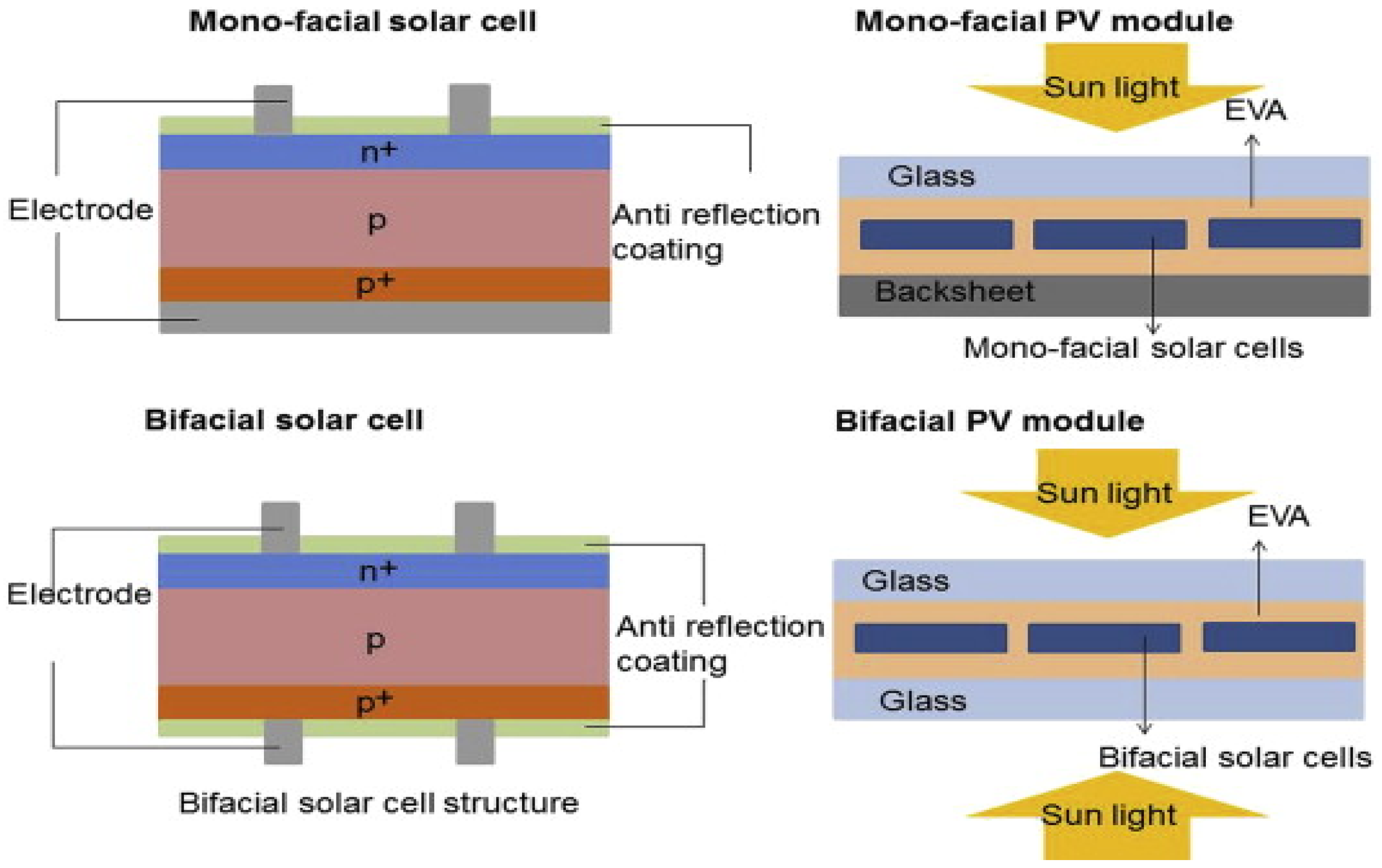
Bifacial solar modules have been studied since the very beginning of PVs. Unlike the conventional PV modules, bifacial PV modules have the ability to capture the energy from the sun using both sides of the module, as they are able to capture the reflected light from the surface under the module and the surroundings using the rear side [9,10]. Similarly, the presence of the screen-printed rear contact on bifacial PV cells permit sunlight to extend to every active region on the module as depicted in Figure 1 [11]. The existence of bifacial PV technology dates back to the early 1980s. In a report by reference [10], a 50% increase in module output was recorded using special light-concentrating systems and solar panels with bifacial solar cells. Moreover, a study conducted by reference [9] also reported an increase of 40% to 70% and 13% and 35% in module output under cloudy and sunny conditions, respectively, depending on mounting elevation [3].

Most of the existing bifacial module technologies are centered on complex solar cell configuration based on n-type silicon substrates or hetero-junction solar cells. This type of cell is active for both sides. In silicon solar cells, the semiconductor substrate could be n-type or p-type thus forming a polycrystalline of two individual solar panels [12]. The front and back side of a bifacial PV module is made of transparent glass–glass material. The presence of the transparent glass material on the back side of the module makes it possible for the reflected sunray to spread across the cells of the module [13]. This process allows for each module to produce more energy output. Inserting the cells in a glass material protects them against any type of environmental and mechanical effects during installation. This protection ensures long service life, high durability and minimal degradation of the module [4].

Figure 1. Schematic of Monofacial and Bifacial PV Module. Source: [14].

Figure 1. Schematic of Monofacial and Bifacial PV Module. Source: [14].

The only commercially available bifacial PV technology is the silicon solar cell, and it accounts for more than 80% of the total PV market worldwide. The function of the screen-printed silver contacts on most silicon solar cell is to conduct the captured sunlight through to the other cells in order to produce the required energy output. It is estimated that between 3% and 10% of the incident light is lost as a result of the shading of these metal contacts and must be accounted for. Scientists have tried to come up with alternative contact designs with a view to minimize the shading loss and subsequently increase the EY of bifacial PV modules. However, the design model is still at the infancy stage and not many studies have been conducted on parameter optimization of bifacial PV modules as the technology is still evolving [15]. In this study, an optimization model (which takes into consideration the shading loss, surface albedo, module elevation or height, tilt angle, the distance separating the modules and mounting orientation) for estimating and increasing the EY of bifacial PV modules is presented in this study.

1.3. Contributions

This study, therefore, focuses on the optimization of the parameters such as mounting height, albedo and mounting angle that influence the extra EY of solar bifacial modules using the Firefly Algorithm (FA). Consequently, the optimal determination of these parameters will improve the overall performance of solar bifacial modules when implementing them for electricity generation in various applications [9]. The algorithm has shown to be very efficient when applied to solve various engineering optimization problems.

1.4. Organization of The Paper

The introductory part of this study is presented in Section 1 detailing a general background of the study, motivation, literature review and the main contributions. The mathematical modeling of the bifacial PV module parameters are reviewed in Section 2. This is followed by a comprehensive description of the optimization algorithm in Section 3. The methodology of the study featuring the developed optimization model is presented in Section 4. Finally, the results and discussions are presented in Section 5.

2. Mathematical Modeling of Bifacial Module Parameters

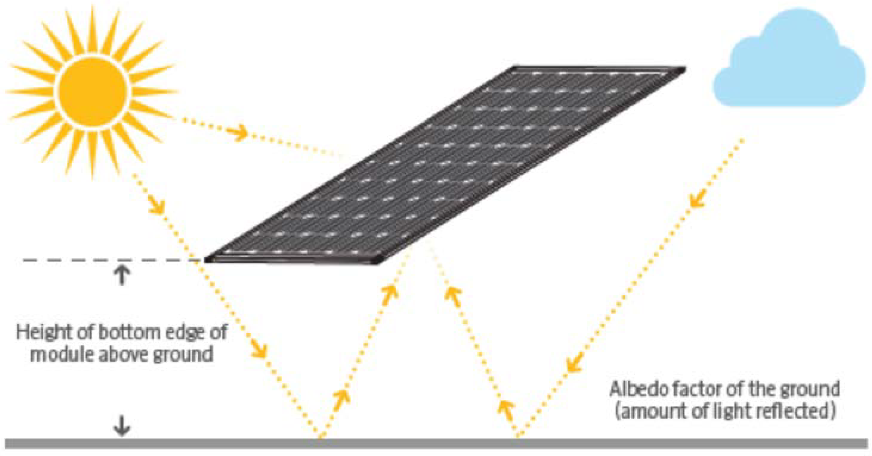
Mathematical modelling is an essential part of any simulation-based design. Figure 2 shows an example of a system using the bifacial solar module. The various parameters used in the modelling of the bifacial PV module in the optimization of the energy yield are presented as follows:

A.

BIFACIALITY (B): Apart from the front side power, a new important parameter was added to the bifacial modules. The transparent and active back sides of bifacial photovoltaic modules enable an additional energy yield, also known as the “energy gain” [8]. The bifaciality, B of the module describes the ratio of the rear side power (P_mpp) to the power generated from the light captured from the front side at Standard Test Conditions (STC) as given in Equation (1) [3].

$$B=\frac{P_{mpp,back}}{P_{mpp,front}}$$

(1)

B.

ALBEDO (λ): The energy output of any PV module depends solely on the amount of sun radiation reaching it: it is thus very important to understand the concept of albedo of the surface where the module is to be installed, as it is primarily responsible for the energy output of the additional side of a bifacial PV module [15]. The albedo, λ describes the reflectivity of a non-luminous surface. It has no dimension and is usually expressed as a percentage. It is evaluated using the ratio of the reflected light (R_L) of the surface to the incident radiation (I_L) as expressed in Equation (2) [16,17].

$$\lambda =\frac{R_L}{I_L}$$

(2)

It should be noted that any increase in the reflectivity of a surface will subsequently lead to a higher albedo value. For instance, a dark material that has the ability to absorb a huge volume of light will subsequently have a low albedo, while a bright surface that is capable of reflecting a large part of the incident sunlight will have a high albedo. The albedo of a surface is one of the important elements that influences the amount of the extra EY [17]. Therefore, the albedo itself is a factor of the type of the material on which the module is mounted [5,17]. The albedo values of some popular materials are presented in

Table 1. Sample Albedo Values of a Few Surfaces. Source: [17].

SURFACE TYPE	ALBEDO CO-EFFICIENT (%)
Ocean ice	(50–70)
New concrete with white portland cement,	(70–80)
New concrete (traditional),	(40–55)
Aged concrete	(20–30)
Desert sand	40
Fresh snow	(80–90)
White acrylic paint	80
galvanized steel	24
Soil (Dark/Wet)	5
Soil (Light/Grey)	40
Green grass	25
Bare soil	17
white paper sheet	(60–70)
polished aluminum	(65–75)
Mirror	(72–85)
Water	(3–100)

.

C.

MODULE HEIGHT (H): The mounting height is the height at which each module is mounted. The mounting height is described in Equation (3) [18,19].

$$H=\frac{H_{ag}}{L_m}$$

(3)

where $H_{ag}$ is the height above ground and $L_m$ is the length of the module.

D.

DISTANCE SEPARATING THE MODULES (A): This parameter also describes the row spacing and it is the distance between each module row. It is expressed in Equation (4) as [5]:

$$A=\frac{D_{br}}{L_m}$$

(4)

where $D_{br}$ is the distance between rows and $L_m$ is the length of the module.

E.

MOUNTING ORIENTATION: This describes the direction the modules are facing. Several approaches have reported a vertical, east-west-facing bifacial modules or south-north-facing modules [17]. In order to maximize the energy yield of this bifacial PV module, it is important to accurately specify the module orientation.

F.

TILT ANGLE: This describes the mounting angle of the module, This parameter varies from site to site, but generally, 3 to 12 degrees more than the monofacial tilt angle have been reported to be quite effective. It should be noted that an increase in the tilting angle will slightly decrease the temperature of the mounting surface [17].

2.1. Modeling the Rear Side Irradiance

Modeling the rear side of a bifacial PV module is a difficult task as several irradiations have to be taken into consideration due to the scattering of the sunray. For the purpose of this study, the rear side is modeled using the view factor method. The equation used in estimating the rear side irradiance was adopted from the work of [20] and is given in Equation (5) as:

$$\begin{gathered} \begin{array}{l}{E}_R=\left(G_b+G_d{A}_i\right)R_{b,f}+G_d\left(1-A_i\right)\left(\frac{1+\cos \left(\beta -180\right)}{2}\right)f\left(\sin \beta -180\right)+\\ \end{array} \\ \hspace{1em}\hspace{1em}\hspace{1em}\hspace{1em} G_d\left(1-A_i\right)\lambda \left(\frac{1-\cos \left(\beta -180\right)}{2}\right)+\left(G_b+G_d{A}_i\right)\lambda \left(\frac{1-\cos \left(\beta -180\right)}{2}-F_{V,R}\right) \end{gathered}$$

(5)

where $\lambda$ is the albedo coefficient, $A_i$ is the anisotropy index, $R_{b,f}$ is the geometric factor, $F_V$ is the view factor, and $f\left(\sin \beta \right)$ is a modulating factor to consider cloudiness and $\beta$ is the tilt angle.

2.2. Energy Yield Estimation of Bifacial PV Module

The extra EY of the bifacial PV module can be described as the percentage of additional energy in the system as a result of the presence of the back side of the module. When the rear side of the module is mounted on a bright material such as shining concrete or white roofing foil, this leads to the reflection of more light back to the module back side; and subsequently leads to an increase in the extra EY. Equation (6) was developed empirically from work performed by [3] and was adopted in this study.

$$E_Y=B\cdot \lambda \left[a\cdot \left(1-\frac{1}{\sqrt{A}}\right)\cdot \left(1-e^{\frac{B-H}{A}}\right)+c\cdot \left(1-\frac{1}{A^4}\right)\right]$$

(6)

where $\lambda$ is the albedo coefficient, $B$ is the bifaciality, $A$ is the row spacing (m), $H$ is mounting height (m), while a and c are constants. Shading factor is neglected for the purpose of this study.

3. Firefly Algorithm

The Firefly Algorithm (FA) is a member of the nature inspired meta-heuristic algorithms. It was inspired based on the flashing behavior of fireflies and the phenomenon of bioluminescent communication. FA has been employed in many optimization problems and has been found to be very effective [15]. Fireflies are capable of producing light that blinks during the night. The light is produced using the abdomen through a process referred to as bioluminescence. This blinking light is specifically used to entice mates and to remind other fireflies about potential predators. The main principle behind the operation of the FA is the global communication among the fireflies. Thus, it has the ability to simultaneously search global and local optimal solutions in any optimization problem [11].

FA generate new solutions using the random movement and attraction among the firefly. Hence, the intensity of the blinking light of each firefly is a function of the objective function of the optimization problem. Once a firefly is attracted to another firefly, this attraction leads to subdivision among the fireflies into smaller groups, with each group swarming around the local models [11,15].

FA employs three ideal rules:

• All fireflies can either be male or female. Hence, regardless of their sex, all fireflies will be attracted to one another.
• The attraction between any two fireflies depends on their blinking intensity, thus a firefly with low blinking light intensity will be attracted to a firefly with high blinking light intensity. It should be noted that the blinking light intensity depends on the distance between the two fireflies. However, if any two blinking fireflies are of the same intensity, this results in random movement.
• Lastly, the light intensity of any firefly is a function of the objective function. For the maximization problem, the light intensity of any firefly is directly related to the value of the objective function.

A group of fireflies moving randomly are initially located in the search space. This initial distribution results in an even distribution of the fireflies. Each firefly moves randomly in the search space and the initial position of each firefly is a possible solution to the optimization problem. Each firefly is made to search in a certain number of dimensions depending on the number of optimization variables [11].

The position of each firefly in the search space is usually represented using a fitness function. This function is used to produce a single numerical output which depends on the quality of the solution to the optimization problem. Once the fitness function of a firefly has been evaluated, a fitness value is assigned to the firefly. The blinking light intensity of each firefly is proportional to the assigned fitness value. Any single firefly with a higher light intensity will attract another firefly with a lesser light intensity [11,15]. The attractiveness of a firefly is a function of the distance separating one firefly to the other. The algorithm then estimates the light intensity of each firefly and updates the position of all the fireflies based on the values obtained. All fireflies are expected to converge to the best possible position on the search space. The firefly with the highest blinking light intensity attracts other fireflies with less blinking light intensity and represents the best possible solution to the optimization problem [15].

In the implementation of the algorithm to various optimization problems, two important issues are usually taken into consideration. The first is the variation of the light intensity of the fireflies, while the second is the formulation of the attraction among the fireflies. This simply means that the attractiveness of any firefly in the search space solely depends on the intensity of the blinking light; which is usually evaluated by the objective function of the problem. Considering the maximization problem, as is the case for this study, the light intensity $I$ of a firefly at a location in the search space ($x$) can be expressed as $I\left(x\right)$ and is relative to the objective function, $f\left(x\right)$.

However, the attractiveness $\phi$ is relative as it varies from one firefly to the other depending on their distance. Hence, it varies with the distance $r_{ij}$ between firefly $i$ and firefly $j$. This means that the farther away a firefly is from another firefly, the lesser the light intensity of the firefly and vice versa. It should be noted that light is also absorbed by the surroundings; therefore, the attractiveness of any firefly is also a function of the degree of light absorption of the medium [11].

Assuming a given search space or medium has a fixed light absorption coefficient ‘γ’, the light intensity, $L$ varies with the distance ‘$r$’ as described by [14] is given in Equation (7).

$$L=L_0{e}^{-\gamma r}$$

(7)

where:

$L_0$ is the initial light intensity.

Since the attraction between any two fireflies is a function of the light intensity, the attractiveness, $\phi$ of a firefly as given by [11] is expressed using Equation (8).

$$\phi ={\phi }_0{e}^{-\gamma r^2}$$

(8)

where:

${\phi }_0$ is the attractiveness at r = 0.

For any two fireflies i and j situated at $x_i$ and $x_j$ respectively, the distance $r_{i,j}$ between them as described by [11] is given as Equation (9):

$$r_{ij=}\left|x_i-x_j\right|=\sqrt{{\displaystyle \sum }_{k=1}^d{\left(x_{i,k}-x_{j,k}\right)}^2}$$

(9)

where $x_{i,k}$ is the kth component of the spatial coordinate $x_i$ and d is the number of distances; assuming d = 2, Equation (10) is further simplified by [11] as:

$$r_{ij}=\sqrt{{\left(x_{i,1}-x_{j,1}\right)}^2+{\left(x_{i,2}-x_{j,2}\right)}^2}$$

(10)

The movement of a firefly i when attracted to another brighter firefly j other than itself as described by [11] is defined using Equation (11).

$$x_i=x_i+{\phi }_0{e}^{-\gamma r_{ij}^2}\left(x_j-x_i\right)+\propto (rand-0.5)$$

(11)

The first term of Equation (11) represents the present location of the firefly, the attraction of the fireflies to light intensity is expressed in the second term and finally, the third term expressed the random movement of any firefly when there are no other fireflies with a higher light intensity. 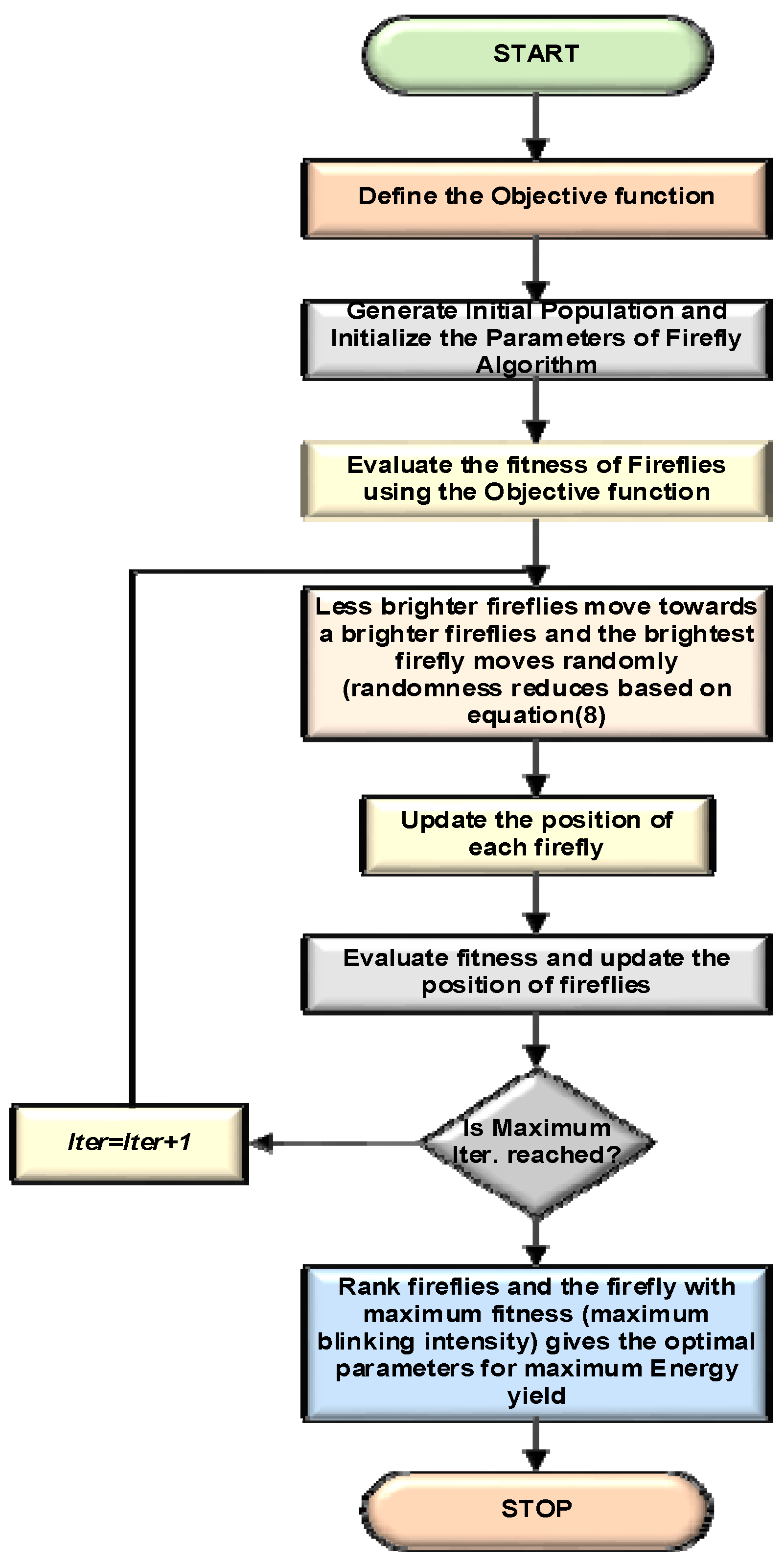The coefficient $\alpha$ is a randomization parameter and rand is a random number generator which is evenly uniformly spread across the search space in the range (0–1), [11,15]. The flow chart of FA is given in Figure 3.

4. Methodology

The extra EY of a bifacial PV module modeling is a very complex task. This is basically due to the need to accurately evaluate the back side irradiance of the module, which is a function of the diffused radiation, the sun altitude, the surface reflective ability, the mounting height and the module tilt angle. These control parameters were adjusted for maximum energy yield estimation. The problem was formulated as a single objective optimization problem. The problem to be maximized is the energy yield of the bifacial PV modules given in Equation (6). It is thus expressed as Equation (12):

$$Max f_x,$$

(12)

where $f_x$ is the objective function to be maximized and is given as Equation (13):

$$f_x=E_Y=B\cdot \lambda \left[a\cdot \left(1-\frac{1}{\sqrt{A}}\right)\cdot \left(1-e^{\frac{B-H}{A}}\right)+c\cdot \left(1-\frac{1}{A^e}\right)\right]$$

(13)

The following boundary conditions are considered in the optimization process.

• Mounting Orientation: This describes the direction of the module during installation and could be either vertical east–west or south–north facing modules.
• Mounting Height: The mounting height is one of the most important parameters to be considered when estimating the extra EY of bifacial PV modules. Studies have shown that the extra EY of bifacial PV modules increases with an increase in the mounting height. Therefore, the mounting height is constrained between its minimum and maximum value as shown in Equation (14).

$$0.5H_{\min }\le H\le H_{\max }$$

(14)

The decision and dependent variables were carefully chosen in order to deal with the various constraints considered in the optimization problem. The decision variables are the bifaciality of the module and the albedo of the surface where the module is to be installed. The albedo was varied in steps of 5% between its lowest and highest values. Dependent variables such as the distance separating the module and the tilt angle were also varied between their maximum and minimum values, respectively. Thus, allowing for the FA to search in the dimension of the search space as given in Equation (15).

$$\{E_Y\to \left\{\lambda ,B,A\right\}$$

(15)

The irradiance of the rear side of the module was estimated using Equation (5), the mounting height was constrained as given in Equation (14), while the mounting orientation was made to alternate between the two directions stated in the constraints for the purpose of this study. Finally, the bifaciality of the module was included in the position of each firefly in the search space as shown in Equation (16).

$$\begin{gathered} X_i=\left[B_{1,i},B_{2,i}\dots \dots \dots B_{N-1,i}\right] \\ \mathrm{for} i=1,\dots \dots \dots N_{pop} \end{gathered}$$

(16)

As a result, the extra EY of the module can be maximized. The possibility of the model violating its limitation was controlled by introducing a penalty factor to penalize the mounting direction and the mounting height as expressed in Equation (17). This is necessary to ensure quality solutions are produced.

$$P_H^{\lim }=\{\begin{array}{l}{P}_{H,\max }; P_H>P_{H,\max }\\ P_{H,\min }; P_H<P_{H,\min }\\ P_H, else,\end{array}$$

(17)

4.1. Fitness Function

The fitness function of all the solutions was determined using the objective function of the problem and a fitness value was assigned to each of the firefly. Consequently, the fitness function (FV) considering the objective function and the sum of penalty terms is expressed in Equation (18).

$$F{V}_i={\displaystyle \sum _{s=1}^{N}f\left(x\right)}+PF$$

(18)

4.2. Implementation of FA for Energy Yield Optimization of Bifacial PV Module

The entire search procedure of the proposed FA model for the optimal EY of the bifacial module is described as follows:

Step 1: Initialize the population of Firefly Algorithm with $N_{pop}$ possible solutions.

Step 2: Estimate the dependent variables for solution i using Equation (6).

Step 3: Determine the penalty term using Equation (17).

Step 4: Evaluate the fitness function $FV$ using Equation (18).

Step 5: Set the solution with the highest fitness as the best solution and denote it as $X_{Gbest}$ and begin the iteration $\left(iter=1\right)$.

Step 6: Generate new solution $X_{ij}^{new}$ for solution $i$.

Step 7: Estimate the fitness function for all new solutions and set the solution with the highest fitness value as $X_{Gbest}^{new}$.

Step 8: If $i=N_{pop}$, proceed to the next step, otherwise set $\left(i=iter+1\right)$ and start again at step 4.

Step 9: Compare the new solutions $X_i^{new}$ to the old solutions $X_i$ and retain the better solutions.

Step 10: Select the best solution among the new solutions and identify them as $G_{best}$. The firefly with the highest light intensity represents the best solution to the optimization problem.

Step 11: Check if iteration count is equal to the maximum iteration $N_{iter}$ and stop the algorithm, otherwise set $iter=iter+1$ and start at step 5.

5. Results and Discussion

The results of the simulations for estimating the specific energy yield are presented in this section. The optimization was confined to two directions: east–west facing modules and south–north facing modules. Figure 4 shows the various energy yield values of the bifacial modules at varying values of albedo, bifaciality of 65%, 25° tilt angle, row spacing of 2.5 m with a vertical south–north orientation. From the results of Figure 4, it was observed that the lowest energy yield was estimated at an albedo coefficient of 5% with an energy yield value of 5.25%. The highest energy yield was estimated at an albedo coefficient of 100% with an energy yield value of 41.50%.

The results of Figure 5 also revealed the various energy yield values of the bifacial modules at varying values of albedo coefficient, bifaciality of 65%, 25° tilt angle and row spacing of 2.5 m with a vertical east–west orientation. It was observed that the lowest energy yield was estimated at an albedo coefficient of 5% with an energy yield value of 10.25%. The highest energy yield was estimated at an albedo coefficient of 100% with an energy yield value of 42.50%. Moreover, the results also showed that for the two orientation states, an increase in the mounting height at the same value of the albedo coefficient, gradually increases the energy yield. However, an inflexion point is reached at a mounting height of 0.5 m, when the extra EY only increases slightly irrespective of the continuous increment in the mounting height. Finally, at a mounting height of 1 m above the ground, the extra EY reaches its saturation point.

From the result shown in Figure 5, it was also observed that the energy yield values obtained from the vertical east–west orientation were better than the additional energy yield values obtained when the optimization was confined to the vertical north–south orientation. Interestingly, simulation results showed that the vertical east–west orientation outperformed the vertical south–north orientation by up to 4.5% within 25° tilt angle, 2.5 m row spacing, 65% bifaciality, 1 m mounting elevation and an albedo coefficient of 100%. This is attributed to the contribution of self-shading of the albedo surface which minimizes the production of extra EY from the back side of the module.

6. Conclusions

The extra EY of the bifacial module is largely dependent on conditions of the environment where the module is to be installed; most especially the mounting height and the albedo of the surface otherwise known as the ground conditions beneath the module. These parameters were optimized to maximize the extra EY of bifacial PV modules. The optimization was confined to two orientation states. The albedo coefficients, as well as the mounting height were varied in steps for maximum energy yield estimation. The Firefly Algorithm was used for the optimization process.

Simulation results revealed that the vertical east–west orientation state offers a higher additional energy yield than the vertical south–north orientation state. It was also observed that self-shading due to the albedo light minimizes the production of the extra EY in the south–north orientation state. However, self-shading is less significant for the vertical east–west orientation and thus produce more extra EY, and should be encouraged when configuring bifacial PV modules for electrical energy production. The minor changes in the extra EY values between the two orientation states reflect the fact that mounting elevation is responsible for the self-shading of bifacial modules. Furthermore, findings also showed that the albedo of the surface plays a significant role in the estimation of the extra EY of bifacial modules.

The developed model will not only assist installers to choose between the two orientation states for maximizing the additional energy yield of bifacial modules for a given location and elevation, it will also help ensure that accurate measures are put in place when considering the configuration parameters of bifacial modules for electrical energy production at the lowest cost of electricity. Future work should be carried out on the optimal configuration of bifacial modules for energy production and be compared with the optimal design configuration of their monofacial counterparts taking into consideration the levelized cost of electricity (LCOE).