Abstract
The main flow could be unsteady in flow fields of film cooling for several reasons such as flow interactions between the rotor and the stator in the turbine. Understanding the characteristics of the film-cooling flow with an unsteady flow is important in the design of gas turbines. The effects of 36-Hz pulsations in the main flow on the streamwise velocity distributions, turbulence statistics, and temperature fluctuations in the film-cooling flow from a cylindrical hole with an orientation angle are investigated by numerical methods. Large-eddy simulation (LES) results match the experimental data with an acceptable accuracy, whereas the Reynolds-averaged Navier–Stokes simulation (RANS) results show large deviations with the experimental data and the LES results. Under 36-Hz pulsations, the URANS results predict a weaker streamwise velocity of the coolant jet that blocks the main flow compared with the LES. With 36-Hz pulsations at the time-averaged blowing ratio of 0.5, urms, the root mean squared fluctuating velocity in the streamwise direction around the coolant core increased due to intensive mixing, and vrms, the root mean squared fluctuating velocity in the wall-normal direction, increased along the trajectory of the injected coolant. Moreover, wrms, the root mean squared fluctuating velocity in the spanwise direction, increased around the wall compared to those at a steady state. The dimensionless temperature fluctuations increased in the region of the core of the coolant compared with those at a steady state. When the orientation angle was 30°, the distribution of the results moved in the z-direction; however, the overall trend was similar to that of a simple angle.
1. Introduction
Gas turbine efficiency can be increased by increasing the turbine inlet temperature [1]. However, the temperature of the turbine blade surface should be kept below an acceptable limit to avoid damage to the blade. Film cooling is a popular cooling method used for turbine blades. The coolant is injected through the holes on the turbine blade surface and protects the surface from the hot main flow. As numerical methods, the Reynolds-averaged Navier–Stokes simulation (RANS) and large-eddy simulation (LES) are widely used. It is known that the LES method predicts the mixing between the main flow and the cooling air more accurately than RANS models; however, the computational cost of an LES simulation is much higher than that of a RANS simulation [2,3].
There have been many numerical studies conducted to understand film cooling when the main flow is steady. Walters and Leylek (2000) used the RANS standard k-ε model to simulate the film cooling on a flat plate and showed that the reattachment of the coolant in a narrow field was not accurately predicted at high blowing ratios [4]. More specifically, the RANS overpredicted the ηc and underpredicted the coolant spreading in the spanwise direction. Tyagi and Acharya (2003) conducted an LES for the film cooling on a flat plate [5]. They demonstrated that not only could the LES produce better predictions of η compared with RANS but also accurately predict coherent structures generated by the film-cooling injection. Rozati and Tafti (2007) investigated the effect of M on η and the heat transfer coefficient with an LES [6] and found that if M was increased, a more turbulent shear layer was generated and η decreased while the heat transfer coefficient increased. Na et al. (2007) investigated the effects of using a ramp through a RANS realizable k-ε model, demonstrating that a ramp located upstream of the film-cooling holes increased η because the ramp caused the interaction between the mainstream and the coolant to occur further away from the wall, rendering the formation of a horseshoe vortex weak [7]. Johnson et al. (2011) studied the effects of the ratio of the hole length (L) to the hole diameter (D) for a cylindrical hole, momentum ratio of the coolant injection, and grid resolution on η using a realizable k-ε model [8] and showed that when the coolant jet had a high momentum and small L/D ratio, η decreased due to the increase in coolant jet lift-off. Bianchini, Andrei, Andreini and Facchini (2013) modified RANS turbulence models and compared the results with conventional two equation RANS models and experimental data [9]. They showed that standard RANS models failed to predict η accurately due to the assumption of isotropic turbulence. Yu and Yavuzkurt (2020) modified the DES model by carrying out the correlation for anisotropic eddy viscosity to obtain better film cooling simulations [10]. They stated that their modified model improved the spreading of the coolant in the spanwise direction compared to the original DES model. Zamiri, You, and Chung (2020) investigated optimum geometry of the hole of the laidback fan-shape in order to improve the cooling performance by using LES [11]. They investigated the effects of three parameters (the metering length, forward expansion angle, and lateral expansion angle) and η from the hole of the optimum geometry was raised by around 50%. According to numerous numerical studies, when an orientation angle was implemented and the coolant was injected in the spanwise direction, η improved. Lee et al. (1997) experimentally investigated the effects of the orientation angle β ranging from 15° to 90° on film-cooling performance [12]. They showed that the counter-rotating vortex pair became asymmetry when the orientation angle was 15° and the vortex pair became a single vortex when the orientation angle was 30°. Jung et al. (1999) also investigated the variations in η with the orientation angle by the experiment [13]. When a compound angle was adopted, η increased from 20% to 80% and it depended on the blowing ratio and the orientation angle.
Another aspect to consider involves the possibility that the main flow could be unsteady in flow fields of the film cooling due to potential flow interactions between the rotor and the stator in the turbine, shock waves, passing wakes, or freestream turbulence [14]. Understanding the variations in η with an unsteady main flow is important in the design of gas turbines. However, there have been few studies showing effects of an unsteady flow on cooling performance. Coulthard, Volino, and Flack (2000) experimentally studied the effects of coolant pulsation on η [15]. They reported that when the jet pulsation frequency is increased, η decreased and the film-cooling performance was maximized when the blowing ratio was 0.5. Nikitopoulos et al. (2009) numerically presented the effects of a coolant jet pulse on film cooling and showed that η could be increased by the pulsation of the coolant jet [16]. Additionally, they found that the frequency and duty cycle of the pulsation, as well as the blowing ratio, are the main parameters affecting η. A simple pulse was used as the instability pattern in the coolant flow; however, the sinusoidal form is more similar to a realistic instability pattern. Seo et al. (1998) experimentally investigated the variations in η with the sinusoidal pulsations of the main flow at the frequencies of 2, 16, and 32 Hz [14]. They showed if the frequencies of the pulsations were raised when the blowing ratio was 0.5, η decreases and the heat transfer coefficients increase. Jung, Ligrani, and Lee (2001) studied the effects of sinusoidal pulsations in the main flow on η experimentally [17]. They presented the flow structures of the coolant, as well as the Reynolds stresses at the frequencies of 0 to 32 Hz for M = 0.5, showing that if the frequencies are increased, the variations in η with the flow structures increase. El-Gabry and Rivir (2012) investigated the effect of coolant jet pulsation on the leading edge model by the experiment and stated that η was reduced compared to that at 0 Hz [18]. Behrendt and Gerendas (2012) studied the effects of flow pressure fluctuations in the main flow on η of double skin liners at M = 1.7 to 5.8 experimentally [19]. They showed that the pressure oscillations decreased η. Moreover, they found that the flow pressure oscillations highly affected η of a material having lower thermal conductivity.
This study investigates the effects of a cylindrical hole system on a flat plate with orientation angles of 0° and 30° under 36-Hz flow pulsations at the time-averaged M of 0.5 on the turbulence statistics of the film-cooling flow. The LES results are compared with the results of the Reynolds-averaged Navier–Stokes (RANS), URANS, as well as available experimental data. More specifically, the time-averaged temperature contours, time-averaged streamwise velocity distribution, and time-averaged turbulence statistics including urms, vrms, wrms, Reynolds stress such as uv, and uw, and temperature fluctuations are investigated. The film-cooling effectiveness and temperature contours under 36-Hz pulsations are demonstrated in a previous study [20].
2. Numerical Method
For the LES and RANS calculations, ANSYS Fluent v.19 [21] was used and Pointwise v.18 [22] was used for mesh generation. Figure 1 shows the procedure of CFD analysis.
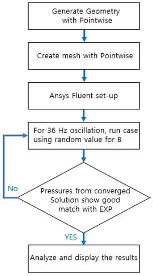
Figure 1.
Procedure of CFD analysis.
For the sub-grid scale model, the Smagorinsky-Lilly model was selected and the realizable k-ε model was selected for the RANS because they matched the experimental data the best [23]. The time step for the LES was set as 5.55 × 10⁻⁶ s and this was the time for the main flow to convect the length of D with 360 time steps [24,25]. The time step for the URANS with 36-Hz pulsations was set as 5.55 × 10⁻⁴ s and this was the time of the 36-Hz pulsation period divided by 50. For each time step, 10 sub-iterations were added to resolve the data well [21]. The CFD simulation was conducted on a 20-core Intel Xeon Gold 6148 processor and the computation times for the LES and RANS calculations were approximately 2 months and 10 h, respectively.
2.1. Computational Domain and CFD Mesh
Figure 2 shows the details of the cylindrical hole configuration for β = 0° and 30°. The orientation angle, β represents the angle between the x direction and the projected injection vector on the wall. The cylindrical hole is located on the wall with a 35° injection angle as illustrated in Figure 2. Figure 3 displays the computational domains of the cylindrical holes. The hole system geometry is based on those presented in [26] and their experimental equipment is characterized by a row having five cooling holes. However, in this study, only a single hole is adopted to save computational costs, and periodic boundary conditions are applied to the main sides (z = ±1.5D). As shown in Figure 3, the computational domain was extended to 24 times of D downstream and upstream from the center (x/D = 0) of the hole. The diameter of the hole (D) is 20 mm, the ratio of L/D is 4 and the ratio of the pitch over D is 3. The geometry was taken from Jung et al. (2001) [26]. Figure 4 shows an overall view of the 3-dimensional mesh of the plane at z/D = 0, the close-up image of the mesh near the hole, and the image of the mesh at the hole exit. The results on the flat plate can be applied to a real turbine blade with minor modifications [27].
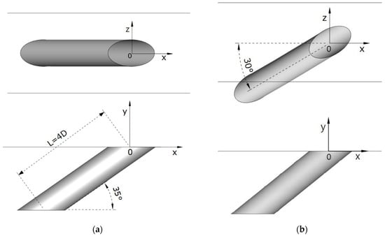
Figure 2.
Details of the cylindrical hole configuration used in the current study with an orientation angle β of 0° and 30°. (a) β = 0°; upper: top view, lower: side view; (b) β = 30°; upper: top view, lower: side view.
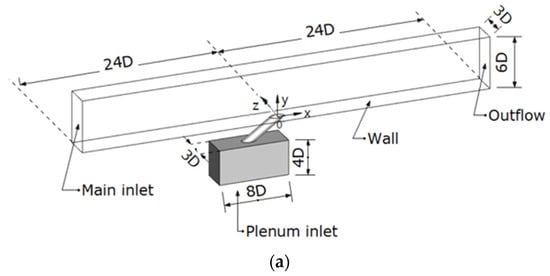
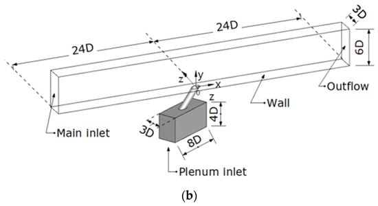
Figure 3.
Computational domain configuration: (a) β = 0°; (b) β = 30°. (a) Orientation angle β = 0°; (b) Orientation angle β = 30°.
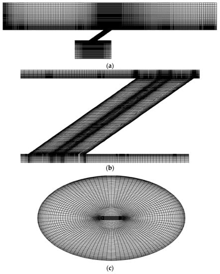
Figure 4.
CFD meshes [20]. (a) View of the mesh at z = 0; (b) Close-up of mesh around the hole; (c) Close-up of mesh at the hole exit.
2.2. Governing Equations and Boundary Conditions
It was assumed that the fluid was incompressible and Newtonian with temperature-dependent variable properties. In this study, the LES, RANS, and unsteady RANS (URANS) were used for the numerical simulations. Generally, the LES requires a much higher computational cost compared with the RANS. However, the RANS approach is limited because all turbulent fluctuations are ensemble-averaged, while the LES method resolves large-scale eddies directly, leading to better predictions of the complex flow [27,28].
2.2.1. Unsteady RANS Approach
The governing equations for the CFD simulations consist of the continuity, momentum, and energy equations. For 36-Hz pulsations, the URANS method is used. The governing equations for the URANS are expressed as [21].
Conservation of mass (continuity equation):
Conservation of momentum:
Conservation of energy:
A closure for the equations could be obtained by the Boussinesq hypothesis as [29]:
where represents the turbulent viscosity and can be expressed as [21]:
2.2.2. LES Approach
The large-eddy simulation (LES) directly resolves large eddies, which are larger than grid spacing. Because mass, energy, and momentum are mostly transported by large eddies, this approach is reasonable [30]. The filtered Navier–Stokes equations for LES are expressed as the following [21]:
The sub-grid scale turbulent stress ( requires modeling and the Boussinesq hypothesis is employed as [21]:
2.2.3. Boundary Conditions
Table 1 shows the boundary conditions of the computational domain. The velocity of the main flow was set as 10 m/s. The time-averaged coolant injection velocity was set as 5 m/s; thus, the time-averaged blowing ratio was 0.5. The velocities were less than Mach 0.3; therefore, the compressibility effect of the fluid was negligible [29,31]. The turbulence intensity of the mainstream at the main inlet was 0.2% and the vortex method was used as the fluctuating velocity algorithm at the main inlet, where the temperatures of the main flow and the coolant were 313 K and 293 K, respectively. The temperature at the main inlet was 293 K and the plenum inlet at the inlet was 313 K, similar to the study in [26], since equally heating the cooling air was easier than equally heating the main flow.

Table 1.
Boundary conditions.
The velocity profile of the main flow at the main inlet was spatially uniform and is expressed as:
Vmain flow = A sin(2πft) + 10 m/s
Table 2.
Value for A in Equation (1).
The velocity profile of the coolant at the plenum inlet was spatially uniform and is expressed as:
where C represents the plenum inlet velocity at steady state (0 Hz). When a sinusoidal pulsation of the main flow was applied to the main inlet, a pulsation with the same frequency was also generated in the coolant at the plenum inlet because the pulsation of the pressure difference between the static pressure near the hole inlet and the static pressure near the hole exit is generated by the pulsation in the main flow. The values of B, the amplitudes of the plenum inlet velocity pulsation in terms of frequency, and the Strouhal number are not reported; however, the plots for the pressure difference variations for 36 Hz are shown in [26]. The values of B were predicted by matching the variation plots by the trial-and-error method as seen in Table 3.
Vplenum inlet = B sin(2πft) + C m/s
Table 3.
B and C values in Equation (2).
2.3. Validation of Numerical Methods
The CFD results were validated by experimental results from [26]. For the mesh sensitivity test, the values for ηc, the centerline (z = 0, y = 0) film cooling effectiveness when the orientation angle β was 0° at steady state with M = 0.5 based on the LES Smagorinsky-Lilly model are illustrated in Figure 5. Five meshes were tested and the specifications for each mesh are indicated in Table 4. The results for the 2.04 million cells are almost the same values of ηc as those for the finer meshes. Therefore, the 2.04 million hexahedron cells were selected for the CFD simulations. The y+ value of the first cell above the wall was less than 2 as illustrated in Figure 6 and there were layers of 25 cells up to y+ = 30.
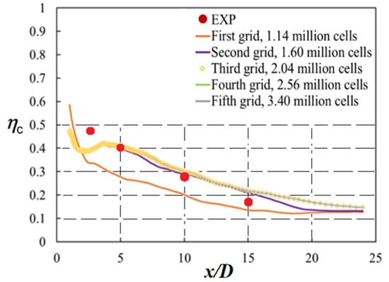
Figure 5.
Comparison of ηc values for the grid sensitivity test based on the LES Smagorinsky-Lilly model [20].
Table 4.
Specifications of mesh arrangements in the crossflow block for the mesh sensitivity test.
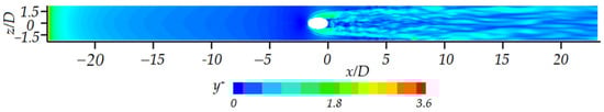
Figure 6.
Contour of y+ on the wall for the mesh of 2.04 million cells.
3. Results and Discussion
3.1. Contours of the Time-Averaged Effectiveness on the Wall
Figure 7 shows the time-averaged η on the wall for β = 0° and 30° at 0 Hz and flow pulsations of 36 Hz at the time-averaged M of 0.5 and 1.0. These contours are compared with the contours obtained through the experimental data in [26], and it can be observed that as x/D increases, η decreases in all cases due to the mixing generated between the main flow and the jet. The film cooling for β = 30° shows better performance than that for β = 0°. When β was 30°, the cooling air was injected at a lateral velocity, increasing η by promoting the spanwise spreading of the cooling air on the wall. The counter rotating vortex pair (CRVP) became asymmetric, and the intensity of the vortex pair was weakened [20]. When the intensity of the CRVP decreased, the entrainment of the hot main flow under the injectant was weakened, resulting in a more uniform coolant coverage.
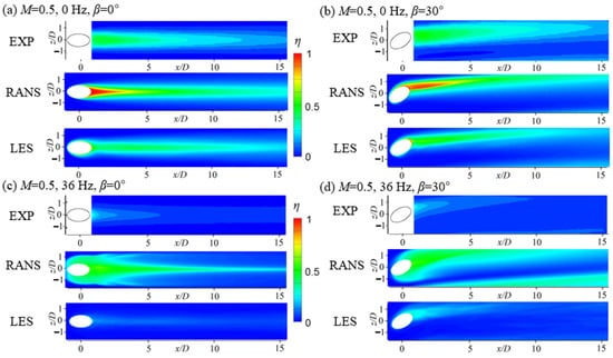
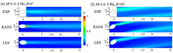
Figure 7.
Time-averaged film-cooling effectiveness contours on the wall compared with the experimental data in [20,26]: (a) M = 0.5, 0 Hz, β = 0°; (b) M = 0.5, 0 Hz, β = 30°; (c) M = 0.5, 36 Hz, β = 0°; (d) M = 0.5, 36 Hz, β = 30°; € M = 1.0, 0 Hz, β = 0°; (f) M = 1.0, 0 Hz, β = 30°.
With an f of +36 Hz, η decreases for all orientation angles. As shown in Figure 7a,b,e,f, at steady state with an M of 0.5 and 1.0, the RANS contours show an over-prediction of η for all orientation angles, particularly near the centerline of the injectant spreading in the narrow region where x/D is less than 5 because of lower mixing between the cooling air and the main flow. The RANS underpredicted the dissipation and lateral spreading of the coolant. The LES contours show that the spread of the injectant in the z-direction on the wall was higher than that of the RANS results. As shown in Figure 7c,d, under the flow pulsation of 36 Hz, the contour of η predicted by URANS also shows a large deviation from the experimental contour. The contours illustrate that the coolant spreading was drastically overpredicted in the narrow region around the hole exit compared with the contours obtained by the experiment. The contours obtained by the LES show a better agreement with the experimental data under the flow pulsation of 36 Hz than at steady state. Thus, it is recommended to conduct an LES rather than a URANS to obtain η under unsteady flow even though LES calculations are much more expensive compared with RANS simulations.
3.2. Time-Averaged Temperature Contours on the Streamwise-Normal Planes
Figure 8 shows the contours for the time-averaged dimensionless temperatures on the streamwise-normal plane at x/D = 2.5 for the orientation angle β of 0° and 30° at 0 Hz and with 36-Hz pulsations at the time-averaged M of 0.5 and 1.0. compared with those from the experimental data in [26] at steady state and at M = 1.0. In the experimental contours, there are no data near the wall since the cold wire could not measure the data near the wall; however, the numerical results can provide some answers. As shown in Figure 8c,d, the shapes of the coolant predicted by the LES show more similar predictions to those in the contours of the experiment compared with the RANS or URANS, especially under 36-Hz pulsations. The shape of the coolant obtained by the URANS under 36-Hz pulsations is quite different from that obtained by the LES or experimental results.
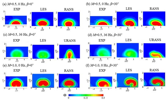
Figure 8.
Time-averaged dimensionless temperature contours on the plane at x/D = 2.5 compared with the experimental data in [20,26]: (a) M = 0.5, 0 Hz, β = 0°; (b) M = 0.5, 0 Hz, β = 30°; (c) M = 0.5, 36 Hz, β = 0°; (d) M = 0.5, 36 Hz, β = 30°; (e) M = 1.0, 0 Hz, β = 0°; (f) M = 1.0, 0 Hz, β = 30°.
At steady state, as shown in Figure 8a,b,e,f, the maximum dimensionless temperatures of the coolant core obtained by the RANS are similar to that predicted by the LES or experimental data, whereas with 36-Hz pulsations, the maximum dimensionless temperatures of the coolant core predicted by the URANS are overpredicted because the URANS underpredicted the mixing intensity between the main flow and the injectant during the flow pulsation. In Figure 8b,d,f, the contours for the orientation angle β of 30° obtained by the experiment in [26], LES, and RANS show that the coolant is inclined and the contact area of the coolant with the wall is increased because the CRVP changes into a single vortex [20], leading to the increase in the film cooling effectiveness on the wall.
3.3. Time-Averaged Streamwise Velocity Contour
Figure 9 shows the normalized streamwise velocity distributions on the streamwise-normal plane at x/D = 2.5. Figure 9a illustrates a comparison of the distribution obtained by the LES, RANS, and the experiment at steady state with M = 1.0 to verify the CFD results. The CFD results provided the velocity distributions for the region below y/D = 0.2, the area for which data could not be measured experimentally. The injectant acts as an obstruction and creates a region of decreased streamwise velocity downstream of the cooling holes. The core of the coolant is indicated in blue with a normalized streamwise velocity of less than 0.7. In the figure, the contour shape of the LES is similar to that of the experimental data in [32], while the RANS simulation results in a coolant jet that blocks the main flow more weakly than in reality.
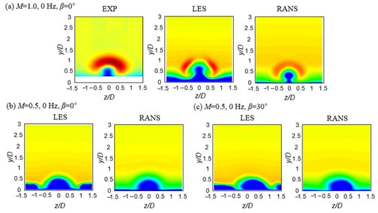
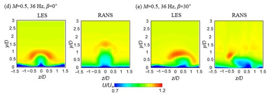
Figure 9.
Time-averaged streamwise velocity contour at x/D = 2.5 for the streamwise film cooling compared with the experimental data in [32] at M = 1.0: (a) M = 1.0, 0 Hz, β = 0°; (b) M = 0.5, 0 Hz, β = 0°; (c) M = 0.5, 0 Hz, β = 30°; (d) M = 0.5, 36 Hz, β = 0°; (e) M = 0.5, 36 Hz, β = 30°.
Moreover, the LES predicted the high streamwise velocity region indicated in red more accurately than the RANS. In the RANS results, the height of the coolant core is smaller than that of the LES and experimental results because the RANS underpredicts the injectant jet lift-off compared with the LES. In the RANS contour, the thickness of the coolant in the region between 0.5 ≤ |z/D| ≤ 1.5 is less than that of the LES results because the RANS predicts a weaker interaction of the coolant with the coolant in the virtual neighboring rows obtained by the periodic boundary conditions on the main sides compared with that of the LES. Moreover, the streamwise velocity gradients in the shear layer predicted by the RANS are smaller than those obtained by the LES, which are similar to those of the experimental data. Figure 9b shows that the injectant jet lift-off at M = 0.5 is not as strong as that at M = 1.0 and the streamwise velocity gradients in the shear layer predicted by the RANS at M = 0.5 are smaller than those obtained by the LES at M = 1.0. In addition, in the RANS results, the thickness of the coolant in the region between 0.5 ≤ |z/D| ≤ 1.5 is less than that in the LES results. When the orientation angle β was 30°, as shown in Figure 9c, the interaction of the coolant with the virtual coolant in the neighboring row became stronger than that for the simple angle in the LES results. However, in the RANS results, the interaction was still weak, similar to that for the simple angle. As shown in Figure 9d,e, under the flow pulsation of 36 Hz, the shape of the normalized streamwise velocity distributions obtained by the LES is quite different from that predicted by the URANS. The URANS result predicted a coolant jet that blocks the main flow more weakly than the LES, similar to the previous cases. Additionally, the streamwise velocity gradients in the shear layer predicted by the LES and URANS are smaller than those at steady state with M = 0.5 because of the intensive mixing between the injectant and the main flow during the pulsation.
For all cases with the orientation angle β of 0°, both the LES and RANS results show that the largest and smallest boundary layer thickness occurred at z/D = 0 and approximately z/D = 0.5, respectively. Therefore, the maximum heat transfer coefficient is expected to occur at approximately z/D = 0.5 and the minimum heat transfer coefficient is expected to occur at z/D = 0 [33].
3.4. Turbulence Statistics
Figure 10 shows the contours of each component of the turbulence intensity at the streamwise-normal plane at x/D = 2.5 obtained by the LES with M = 0.5 and 1.0 at steady state and with 36-Hz pulsations for the orientation angles β of 0° and 30°. The contour from the experiment conducted by Burd et al. [34] at steady state with M = 1.0 for the orientation angle β of 0° validates the LES results. The LES-obtained contours are similar to those in the experiment under the same operating conditions. The RANS k-ε turbulence model severely underpredicts the turbulence intensity, and the maximum values of the normalized urms, vrms, and wrms do not exceed 10% of the values in the LES results, and the contours of the RANS could not be shown within the contour range in LES and they are not included. As shown in the figure, in the experimental data, the turbulence intensity below y/D = 0.2 could not be measured; however, the LES contours show the contours of urms, vrms, and wrms below y/D = 0.2, which are highest around the core area of the coolant.
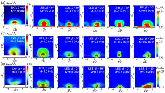
Figure 10.
Normalized turbulence intensities at x/D = 2.5 compared with the experimental data in [27]: (a) urms/U∞; (b) vrms/U∞; (c) wrms/U∞.
As shown in Figure 10a,c, urms and wrms do not converge to zero at the wall but show high values along the wall, whereas vrms converges to zero at the wall. When the orientation angle β was 30°, the CRVP changed into a single vortex and the contours of the normalized urms, vrms, and wrms became asymmetric and the contours of the coolant core moved in the +z-direction. However, the overall trends of the distribution are similar to those of the simple angle β = 0° and the maximum values of the normalized urms, vrms, and wrms are also similar to those of the simple angle. At M = 0.5, the overall distributions of the components of the turbulence intensities are downsized compared with those at M = 1.0. When the pulsation of 36 Hz was applied to the flow, the values of urms around the coolant core increased, and the change in the contour is attributed to the periodic change in the blowing ratio, as shown in Equation (10), resulting in periodic variations in the injection velocity of the coolant. The values of wrms around the wall increase in Figure 10c. However, the contour of vrms does not show any significant differences from that at steady state due to the existence of the wall. When the orientation angle β is 30° and the pulsation of 36 Hz is applied, the overall trends of the contours are similar to those of the simple angle (β = 0°); however, the values of wrms near the wall are higher than those in the case with the simple angle.
Figure 11 shows the contours of the Reynolds stress u’v’ and u’w’ on the streamwise-normal plane at x/D = 2.5. As shown in Figure 11a, at M = 1.0, the Reynolds stress below y/D = 0.2, which could not be measured experimentally, was predicted by the LES, and the distributions of the peaks for u’v’ and u’w’ are similar to those in the experimental data of Kaszeta et al. [32]. However, the peaks shown in the shear layer over the coolant core in the LES results are weaker than those in the experimental data because the turbulence intensity of the freestream is much lower in the LES (0.2%) than that in the experiment (12%). Figure 11b shows that the Reynolds stress in the coolant jet core obtained by the LES for the orientation angle (β) of 0° at M = 0.5 decreases compared with that at M = 1.0; however, the shape of the distribution of the Reynolds stress is almost the same as that at M = 1.0, except for the shear layer over the coolant core. At steady state with M = 0.5, the Reynolds stress over the coolant core is weakened compared with that at M = 1.0. In Figure 11c, if the pulsation of 36 Hz is applied to the flow, the values of the Reynolds stress are increased drastically around the core of the coolant and the peaks of the Reynolds stress in the shear layer over the coolant core appear. When the orientation angle (β) of 30° is adopted, the cooling air is injected at a lateral velocity and the Reynolds stress is generated around the single vortex [33].
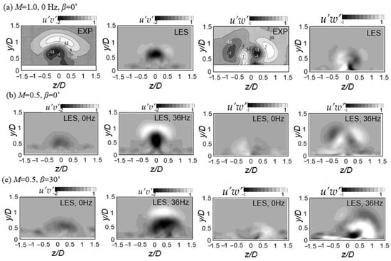
Figure 11.
Contours of Reynolds stress for the plane at x/D = 2.5: (a) EXP [32] and LES at M = 1.0, 0 Hz, β = 30°; (b) LES at M = 0.5, β = 0°; (c) LES at M = 0.5, β = 30°.
Figure 12 shows the contours of the urms and vrms of the turbulence intensity and the Reynolds stress uv for the plane at z = 0 obtained by the LES at steady state and with flow pulsations of 36 Hz at M = 0.5 and 1.0 for the orientation angle β of 0° in comparison with the experimental data from a study by Coletti et al. [35] at M = 1.0. In Figure 12a–c, the LES-obtained results at M = 1.0 are similar to those in the experiment. The LES results illustrate the urms, vrms, and uv below y/D = 0.2, the area of which these values could not be measured experimentally. In Figure 12a, the values of urms obtained by the LES increase around the hole center (x/D = 0) and along the shear layer under the core of the coolant in the region between 1 ≤ x/D ≤ 3 and are not strong in the far field. The LES results match the experimental data with an acceptable accuracy even though the LES results are slightly overpredicted. As shown in Figure 12b, the values of vrms are strong along the injectant and the LES results are slightly overpredicted compared with the experimental results. In the contour of Reynolds stress uv in Figure 12c, the Reynolds stress is strongly generated around the shear layer under the core of the injected coolant downstream of the hole and expands in the streamwise direction with the trajectory of the coolant, while the Reynolds stress generated upstream of the hole does not expand in the streamwise direction.
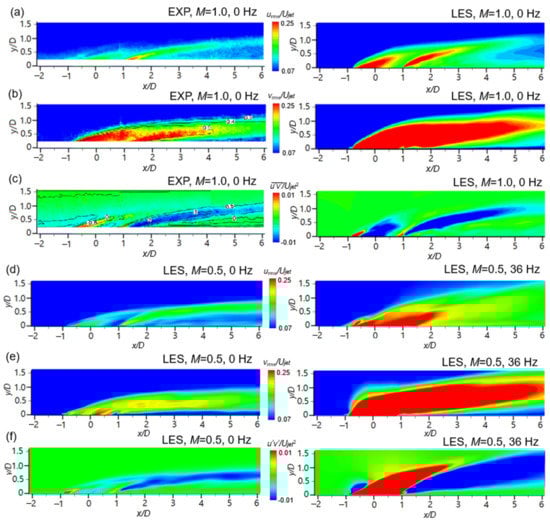
Figure 12.
The dimensionless urms, vrms, and uv at z/D = 0 compared with the experimental data of Coletti et al. [35]: (a) urms/U∞ at M = 1.0; (b) vrms/U∞ at M = 1.0; (c) wrms/U∞ at M = 1.0; (d) urms/U∞ at M = 0.5; (e) vrms/U∞ at M = 0.5; (f) wrms/U∞ at M = 0.5.
As can be observed in Figure 12d–f, at steady state with a blowing ratio of 0.5, the distributions for urms, vrms, and uv appear to be similar to those at M = 1.0, but the values are lower. If the pulsation of 36 Hz is applied to the flow, the area with high values of urms, vrms, and uv obtained by the LES becomes much larger than that at steady state with M = 0.5. The definition of the Strouhal number is Sr = and this value is the ratio of the time needed for the injectant to pass through the hole to the time of a pulsation cycle. Thus, if the Strouhal number is greater than 1, it implies that the coolant is greatly affected by the pulsation while the coolant passes through the hole [14]. Therefore, under the pulsation of 36 Hz, the trajectory of the injectant differs considerably from that at steady state, and the mixing intensity is increased, leading to higher values of urms, vrms, and uv than the values at steady state with M = 1.0. Specifically, urms increases around the center of the hole and the trailing edge of the hole. vrms increases along the trajectory of the injected coolant. Moreover, the height of high value of vrms in the region between −1 ≤ x/D ≤ 0 increases and the shape of high value of vrms becomes blunt. Additionally, the values of vrms are the lowest around the wall at x/D > 2, the values of uv around the injected coolant increase, and the signs of the values at the main flow inlet and the outlet are opposite.
Figure 13 shows the contour of the Reynolds stress uv on the plane at y/D = 0.5 near the wall. As shown in Figure 13a, the LES-obtained distribution of uv at steady state with M = 1.0 is similar to that of the experimental data in [35], except for the streak of Reynolds stress generated around the hole. Two main blue streaks and one red streak are generated by the CRVP; however, the streak of uv generated around the hole in the experimental data is not predicted by the LES. In Figure 13b, the Reynolds stress at steady state with M = 0.5 decreases compared to that with M = 1.0; however, the trend of the distribution is almost the same with two main blue streaks and one red streak generated. The secondary peaks shown for M = 1.0 are not shown for M = 0.5. Figure 13c shows that when the pulsation of 36 Hz is applied to the flow, the secondary peaks become stronger while the main peaks are weakened. For the orientation angle of 30° at steady state with M = 0.5, the primary streaks become asymmetric and the blue streak is weakened, while the red streak becomes stronger. Similarly, when the pulsation of 36 Hz is applied, the secondary peaks also become strong, similar to the results for the simple angle; however, the main blue streak is weakened.
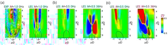
Figure 13.
Reynolds shear stresses along the plane of y/D = 0.5: (a) EXP [35] and LES, M = 1.0, β = 0°, 0 Hz; (b) LES, M = 0.5, β = 0°; (c) LES, M = 0.5, β = 30°.
3.5. Temperature Fluctuations
Figure 14 shows the dimensionless temperature fluctuations θrms for the plane at x/D = 2.5 obtained by the LES. In the RANS results, θrms is too small to be fitted within the same contour range, and only the LES results are shown in Figure 14. As can be observed in Figure 14a,b, at steady state, θrms is high around the region of the shear layer for the mean temperatures in Figure 8, while the components of the turbulence intensities are high in the region of the core area of the coolant, as observed in Figure 10.
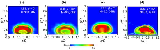
Figure 14.
Temperature fluctuations obtained from the LES at x/D = 2.5 for M = 0.5: (a) β = 0°, 0 Hz; (b) β = 30°, 0 Hz; (c) β = 0°, 36 Hz; and (d) β = 30°, 36 Hz.
When the pulsation of 36 Hz is applied to the flow, θrms in the region of the core of the coolant is also increased compared with that at steady state due to the intensive mixing, which is indicated by the increase in the red area. In the case of the orientation angle β of 30°, the distribution of the temperature fluctuations moves in the z-direction; however, the overall trend is similar to that of the simple angle (β = 0°).
4. Conclusions
The effects of 36-Hz flow pulsations (Sr = 3.62) at the blowing ratio of 0.5 for a cylindrical hole system with the orientation angle of 0° and 30° on the characteristics of the film-cooling flow are studied using the LES and RANS. The following conclusions were derived under 36-Hz pulsations:
- The contours of the time-averaged effectiveness and the dimensionless temperatures of the coolant on the streamwise-normal plane obtained by the LES show a better agreement with the experimental data than with the contours at steady state.
- The streamwise velocity gradients in the shear layer predicted by the LES and URANS are smaller than those at steady state because of the intensive mixing between the coolant and the main flow.
- The URANS results predict a weaker streamwise velocity of the coolant jet that blocks the main flow compared with the LES.
- The values of urms around the coolant core, the center of the hole and the trailing edge of the hole increase as well as the values of wrms around the wall, while the contour of vrms increased along the trajectory of the injected coolant. Additionally, in the contour of uv, the secondary peaks became stronger while the main peaks weakened.
- The dimensionless temperature fluctuations increase in the region of the core of the coolant compared with those at steady state.
- For the orientation angle of 30°, the secondary peaks became stronger, similar to those for the simple angle, although the main blue streak weakened.
- This paper only covered the cylindrical hole, however, the effects of the main flow pulsations on film cooling for the shaped hole such as the forward expansion hole will be covered in future studies. Moreover, the effects for the two sister holes positioned more downstream of the primary hole and the optimized length between the sister hole and the primary hole will be investigated to obtain the best film cooling performance. For the parametric study, the CFD results of this study could be used as the baseline.
Author Contributions
Simulations, S.-I.B.; analysis, S.-I.B. and J.A.; writing, S.-I.B. and J.A.; supervision, J.A. All authors have read and agreed to the published version of the manuscript.
Funding
This work was supported by the Korea Institute of Energy Technology Evaluation and Planning (KETEP) and the Ministry of Trade, Industry and Energy (MOTIE) of the Republic of Korea (No. 1415167167).
Institutional Review Board Statement
Not applicable.
Informed Consent Statement
Not applicable.
Data Availability Statement
Not applicable.
Conflicts of Interest
The authors declare no conflict of interest.
Nomenclature
| D = hole diameter | |
| L = hole length | |
| M = blowing ratio = | |
| P = pitch between holes [mm] | |
| Sr = Strouhal number = | |
| T = temperature [K] | |
| t = time [s] | |
| U = flow velocity [m/s] | |
| u = fluctuating velocity [m/s] | |
| x = streamwise coordinate | |
| y = wall-normal coordinate | |
| z = spanwise coordinate | |
| Greek symbols | |
| β | = orientation angle |
| = angle between the streamwise direction and projected injection vector on the x–z plane | |
| κ = von Karman’s universal constant = 0.41 | |
| = adiabatic film cooling effectiveness | |
| = spanwise-averaged film cooling effectiveness | |
| = density [kg/m3] | |
| τij = sub-grid scale turbulent stress | |
| μt = sub-grid scale turbulent viscosity [kg/(m·s)] | |
| μ = dynamic viscosity | |
| Θ = dimensionless temperature | |
| Subscripts | |
| C = coolant | |
| G = mainstream gas | |
| m = spanwise-averaged | |
| rms = root mean squared | |
References
- Moran, M.; Shapiro, H.; Boettner, D.; Bailey, M. Fundamentals of Engineering Thermodynamics, 8th ed.; Wiley: Hoboken, NJ, USA, 2014; p. 532. [Google Scholar]
- Leedom, D.H.; Acharya, S. Large eddy simulations of film cooling flow fields from cylindrical and shaped holes. In Proceedings of the ASME Turbo Expo 2008, Berlin, Germany, 9–13 June 2008; pp. 865–877. [Google Scholar]
- Baek, S.; Ryu, J.; Ahn, J. Large Eddy Simulation of Film Cooling with Forward Expansion Hole: Comparative Study with LES and RANS Simulations. Energies 2021, 14, 2063. [Google Scholar] [CrossRef]
- Walters, D.K.; Leylek, J.H. Impact of film-cooling jets on turbine aerodynamic losses. ASME J. Turbomach. 2000, 122, 537–545. [Google Scholar] [CrossRef]
- Tyagi, M.; Acharya, S. Large eddy simulation of film cooling flow from an inclined cylindrical jet. ASME J. Turbomach. 2003, 125, 734–742. [Google Scholar] [CrossRef]
- Rozati, A.; Tafti, D. Large eddy simulation of leading edge film cooling: Part II—Heat transfer and effect of blowing ratio. In ASME Turbo Expo 2007; ASME: Montreal, QC, Canada, 2007. [Google Scholar]
- Na, S.; Shih, T. Increasing adiabatic film cooling effectiveness by using an upstream ramp. J. Heat Transfer. 2007, 129, 464–471. [Google Scholar] [CrossRef]
- Johnson, P.; Shyam, V.; Hah, C. Reynolds-Averaged Navier-Stokes Solutions to Flat Plate Film Cooling Scenarios; NASA/TM-2011-217025; NASA: Washington, DC, USA, 1 May 2011. [Google Scholar]
- Bianchini, C.; Andrei, L.; Andreini, A.; Facchini, B. Numerical Benchmark of Nonconventional RANS Turbulence Models for Film and Effusion Cooling. J. Turbomach. 2013, 135, 041026. [Google Scholar] [CrossRef]
- Yu, F.; Yavuzkurt, S. Near-Field Simulations of Film Cooling with a Modified DES Model. Inventions 2020, 5, 13. [Google Scholar] [CrossRef] [Green Version]
- Zamiri, A.; You, S.; Chung, J. Large eddy simulation in the optimization of laidback fan-shaped hole geometry to enhance film-cooling performance. Int. J. Heat Mass Transf. 2020, 158, 120014. [Google Scholar] [CrossRef]
- Lee, S.W.; Kim, Y.B.; Lee, J.S. Flow Characteristics and Aerodynamic Losses of Film-Cooling Jets with Compound Angle Orientations. J. Turbomach. 1997, 119, 310–319. [Google Scholar] [CrossRef]
- Jung, I.S.; Lee, J.S. Effects of Orientation Angles on Film Cooling over a Flat Plate: Boundary Layer Temperature Distributions and Adiabatic Film Cooling Effectiveness. J. Turbomach. 1999, 122, 153–160. [Google Scholar] [CrossRef]
- Seo, H.; Lee, J.; Ligrani, P. The effect of injection hole length on film cooling with bulk flow pulsations. Int. J. Heat Mass Transf. 1998, 41, 3515–3528. [Google Scholar] [CrossRef]
- Coulthard, S.M.; Volino, R.J.; Flack, K.A. Effect of Jet Pulsing on Film Cooling-Part I: Effectiveness and Flow-Field Temperature Results. J. Turbomach. 2006, 129, 232–246. [Google Scholar] [CrossRef]
- Nikitopoulos, D.E.; Acharya, S.; Oertling, J.; Muldoon, F.H. On Active Control of Film-Cooling Flows. In Proceedings of the ASME Turbo Expo, Barcelona, Spain, 8–11 May 2006. GT2006-90051. [Google Scholar]
- Jung, I.S.; Ligrani, P.M.; Lee, J.S. Effects of bulk flow pulsations on phase-averaged and time-averaged film-cooled boundary layer flow structure. J. Fluids Eng. 2001, 123, 559–566. [Google Scholar] [CrossRef]
- El-Gabry, L.A.; Rivir, R.B. Effect of Pulsed Film Cooling on Leading Edge Film Effectiveness. ASME J. Turbomach. 2012, 134, 041005. [Google Scholar] [CrossRef]
- Behrendt, T.; Gerendas, M. Characterization of the influence of moderate pressure fluctuations on the cooling performance of advanced combustor cooling concepts in a reacting flow. In Turbo Expo: Power for Land, Sea, and Air; GT2012-68845; American Society of Mechanical Engineers: New York, NY, USA, 2012. [Google Scholar]
- Baek, S.; Ahn, J. Large Eddy Simulation of Film Cooling Involving Compound Angle Hole with Bulk Flow Pulsation. Energies 2021, 14, 7659. [Google Scholar] [CrossRef]
- ANSYS Fluent Theory Guide Version 19. Available online: https://www.ansys.com/products/fluids/ansys-fluent (accessed on 21 January 2022).
- Pointwise Version 18. Available online: http://www.pointwise.com/ (accessed on 10 October 2021).
- Baek, S.I.; Yavuzkurt, S. Effects of Flow Oscillations in the Mainstream on Film Cooling. Inventions 2018, 3, 73. [Google Scholar] [CrossRef] [Green Version]
- Renze, P.; Schröder, W.; Meinke, M. Large-eddy Simulation of Film Cooling Flows with Variable Density Jets. Flow Turbul. Combust. 2007, 80, 119–132. [Google Scholar] [CrossRef]
- Iourokina, I.; Lele, S. Towards large eddy simulation of film cooling flows on a model turbine blade leading edge. In Proceedings of the 43rd AIAA Aerospace Sciences Meeting and Exhibit, Reno, NV, USA, 10–13 January 2005. No. 2005-0670. [Google Scholar]
- Jung, I.S. Effects of bulk flow pulsations on film cooling with compound angle injection holes. Ph.D. Thesis, Seoul National University, Seoul, Korea, 1998. [Google Scholar]
- Han, J.; Dutta, S.; Ekkad, S. Gas Turbine Heat Transfer and Cooling Technology, 2nd ed.; CRC Press: Boca Raton, FL, USA, 2013. [Google Scholar]
- Farhadi-Azar, R.; Ramezanizadeh, M.; Taeibi-Rahni, M.; Salimi, M. Compound Triple Jets Film Cooling Improvements via Velocity and Density Ratios: Large Eddy Simulation. J. Fluids Eng. 2011, 133, 031202. [Google Scholar] [CrossRef]
- Cengel, Y.; Cimbala, J. Fluid Mechanics, 3rd ed.; McGrawHill: New York, NY, USA, 2014. [Google Scholar]
- Acharya, S.; Leedom, D.H. Large Eddy Simulations of Discrete Hole Film Cooling with Plenum Inflow Orientation Effects. J. Heat Transf. 2012, 135, 011010. [Google Scholar] [CrossRef]
- White, F. Fluid Mechanics, 8th ed.; McGraw-Hill: New York, NY, USA, 2015. [Google Scholar]
- Kaszeta, R.; Simon, T. Measurement of Eddy Diffusivity of Momentum in Film Cooling Flows with Streamwise Injection. J. Turbomach. 2000, 122, 178–183. [Google Scholar] [CrossRef]
- Baek, S.; Ahn, J. Large Eddy Simulation of Film Cooling Involving Compound Angle Holes: Comparative Study of LES and RANS. Processes 2021, 9, 198. [Google Scholar] [CrossRef]
- Burd, S.W.; Kaszeta, R.W.; Simon, T.W. Measurements in Film Cooling Flows: Hole L/D and Turbulence Intensity Effects. J. Turbomach. 1998, 120, 791–798. [Google Scholar] [CrossRef] [Green Version]
- Coletti, F.; Benson, M.; Ling, J.; Elkins, C.; Eaton, J. Turbulent transport in an inclined jet in crossflow. Int. J. Heat Fluid Flow 2013, 43, 149–160. [Google Scholar] [CrossRef]
Publisher’s Note: MDPI stays neutral with regard to jurisdictional claims in published maps and institutional affiliations. |
© 2022 by the authors. Licensee MDPI, Basel, Switzerland. This article is an open access article distributed under the terms and conditions of the Creative Commons Attribution (CC BY) license (https://creativecommons.org/licenses/by/4.0/).