Abstract
Vortex generators are used to overturn the momentum of the flow in the boundary layer, thereby preventing flow separation, and are broadly used in aviation, wind power, heat exchange, and different fields. It has been determined that the capability of an eddy current generator to manipulate the boundary layer is proportional to the intensity of the vortex strength it excites. Although the mathematical notion of vortex strength is very well defined, there are difficulties in figuring out vortex strength in applications. This article proposes a calculation method based on confidence intervals and contour eddy current intensity. Meanwhile, the contemporary overall performance evaluation of vortex generators is frequently obtained in a roundabout way through their consequences on feature factors (e.g., lift coefficients, etc.), and techniques for the direct assessment of a vortex generator’s overall performance are no longer available. To address this situation, the article derives the performance evaluation criterion of the equal height vortex generators, the harmonic intensity factor (), based on the Biot–Savart theorem.
1. Introduction
Because of friction, fluid particles will be slowed down in a small near-wall region, called a boundary layer. Then, the separation will show up after a certain characteristic length. Fluid mechanics will meet an adverse pressure gradient and large energy losses when boundary layer separation occurs, so the control of flow separation remains exceedingly important [1,2]. The principle of the vortex generator taking control of the boundary layer is as follows: through the excitation of the induced vortex, the mainstream fluid’s kinetic energy is accelerated to the boundary layer inside the transfer and enhances the near-wall boundary layer fluid’s energy to achieve the purpose of inhibiting and delaying the separation of the boundary layer. As a passive vortex excitation device, the vortex generator, originally introduced by Taylor [3], is structurally simple and adds little structural complexity, and is broadly used in the aerospace and wind power industries [1,4]. With the trend of large-scale wind turbines and taking into account their strength and structural compatibility requirements, wind turbine blades are widely used in airfoils with a large relative thickness; thus, the boundary layer separation phenomenon on the blade is more obvious, and the need for boundary layer control is more urgently. Meanwhile, the harsh working environment of wind turbines has put a higher demand on the reliability of boundary layer control equipment. The simple structure and reliable performance of vortex generators in the control of wind turbine blades’ boundary layers are increasingly being investigated. Therefore, there is a need for a way to evaluate the advantages and disadvantages of the control performance of vortex generators.
The vortex strength of the induced vortex caused by the vortex generator is an important parameter that has an impact on its flow control performance [5]. The higher the vortex strength of the induced vortex, the faster the fluid kinetic energy transfer rate [5]. The vortex strength in a vortex field is equivalent to the vortex flux through the sectional area, and the vortex strength is defined as:
where J is the vortex strength (vortex flux); is the vorticity; is the unit vector that is normal to the outer micro-element on the surface (A); is the velocity vector of the integral curve (ds); and is the outer boundary curve micro-element of the vortex.
Despite the well-defined mathematical definition of vortex strength, the calculation of the integration curve in the application encountered some difficulties. The current mainstream approach has two calculation methods: one method is to locate the distance between the peak vorticity point and the azimuthal velocity’s maximum point to define the vortex radius to identify the integration curve; the other is to use the vortex distribution to obey the Gaussian distribution [6,7,8,9,10] and determine the vortex radius by calculating the distance from the peak vorticity point to the half-peak vorticity point [11,12] to determine the integration curve. Nevertheless, due to the limitation of sampling accuracy and secondary eddy interference, each of these methods has shortcomings. In this article, the confidence interval method of the probability theory is introduced to integrate the vortex contours to enclose the region for the calculation of vortex size, which excludes the influence of the randomness of sampling and arbitrariness of the region and improves the calculation accuracy.
The control performance of the vortex generator on the boundary layer is proportional to the vortex strength, and a strong correlation between them was found in some research. However, the assessment of vortex generator performance with the aid of vortex strength alone is not sufficient in some situations.
Presently, there is no direct standard for the performance evaluation of vortex generators, and the performance of vortex generators can only be assessed by indirect measures, such as calculating the improvement of the blade lift coefficient or the improvement of the annual power generation of wind turbines [13,14,15]. In flat plate experiments on vortex generators, only the magnitude and dissipation of vortices are mostly explored, and there are no direct arguments to compare the performance of vortex generators. In this paper, we propose a direct evaluation criterion for the performance of an equal height vortex generator based on the Biot–Savart theorem.
2. Mathematical Model
2.1. Calculation Model of Vortex Strength
The shortcoming of the determination of vortex strength via the method of calculating the distance from the peak vorticity point to the maximum point of azimuthal velocity is that the maximum point of azimuthal velocity is induced by both the primary and secondary vortices, causing the method to have the downside of calculating a value that is somewhat higher than the authentic value. The principle of the half-life radius [10,15] calculation method is that the vortex strength is determined by calculating the spacing from the peak vortex point to the half-peak vortex point in view of the fact that the axial vorticity obeys a Gaussian distribution on the detection surface [6,7,8,9], as shown in Figure 1. This approach attempted to eliminate the influence of secondary vortices on the calculation; however, the method considers that the vortices exist within the circle enclosed by the half-life radius (Ruben [16] et al. considered a two-dimensional Gaussian distribution and developed the vortex boundary into an ellipse). However, due to the presence of secondary vortices, the vortex boundary is not a regular graph, so this method is also deficient in terms of calculation accuracy.
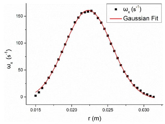
Figure 1.
The sampling points of axial vorticity obey Gaussian distribution.
Under the assumption of Gaussian distribution and based on the theory of the confidence interval in probability theory, the present paper offers a relatively more accurate method to determine the vortex strength.
Let the vorticity sample population X obey Gaussian distribution Let the sampling sample , then the estimates of the moments of , are:
Then, take the random variable T:
The sample obeys t-distribution. From , the interval with a confidence level of 0.9 can be calculated by querying the t-distribution table as []. That is, the vortex radius is no longer the half-life radius, but .
If the vortex strength is calculated according to the half-life radius method, the vortex strength value is obtained by integrating the vorticity in a circle of radius R with the vortex peak point as the center. As a result of the presence of secondary vortices, the main vortex will be squeezed and deformed, so the area is not a positive circle, resulting in errors between the calculated and observed values.
The contour method enables a more accurate determination of the vortex calculation area. From the sample satisfying the Gaussian distribution, the corresponding vortex strength can be calculated by substituting the R into Equation (4), and the range enclosed by the contour of R is the calculated area, which is denoted as A.
Within A, the vortex strength can be computed by Equation (1) as:
2.2. Vortex Generator Performance Evaluation
As mentioned previously, it is flawed to evaluate the vortex generator’s performance in controlling the boundary layer fluid by considering only the vortex strength of the induced vortex. According to the Rankine composite vortex model, the fluid internal to the vortex core has a rigid body rotation, and the fluid outside the vortex core is a potential flow. In other words, the vortex flow velocity outside the vortex core varies and monotonically decreases. By considering the principle of the vortex control of the boundary layer, its effect is mainly to accelerate the kinetic energy exchange of the fluid. This means that the greater the vortex-induced velocity of the fluid close to the blade wall, the greater the vortex’s ability to control the boundary layer. The direction of the induced velocity of the vortex core region on the fluid can be determined according to the right-hand rule, and the magnitude of the induced velocity obeys the Biot–Savart theorem [17]. The velocity induced by the vortex core at point P is , and point P is r from the vortex center. The micro-element segment dl on the vortex beam at a distance R from the point P is shown in Figure 2. The angle between the micro-element segment dl and the line connecting point P to the vortex center is α1. Then, the induced velocity can be determined using Equation (6).
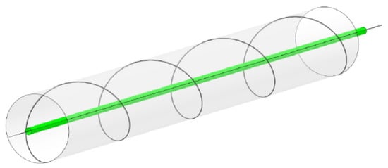
Figure 2.
Diagram of the Biot–Savart’s theorem.
Meanwhile, from the trigonometric relationship, it is obtained that:
Within the angle α1~α3,
If we let the vortex beam have infinite length, the induced velocity can be written as:
The vortex flux within the vortex core is continuous, and the farther the vortex flux’s micro-element segment dl is from the detection surface, the smaller the influence of the micro-element segment on the induced velocity (because the angle α is smaller). Therefore, for the vortex generator with the same height, only the induced velocity of the vortex beam on the detection surface is available to examine the strength of the conditioning capability of the fluid.
From Equations (5) and (9), the calculation of the fluid velocity close to the surface of the blade assumes that the vortex strength is available. However, as mentioned before, different calculation methods calculate different vortex strengths [10,16], which in turn affects the calculation of the induced velocity. To get rid of this issue, considering that the peak vortex ωpeak is convenient to obtain in the experiment or simulation, and the corresponding sampling area is identical, the product of the peak vortex and the sampling area per unit of the grid can be used to replace the detection surface’s vortex strength. Then, based on Equation (9), the induced velocity of the vortex peak on the surface of the object is:
where is the induced velocity of the vortex nucleus on the detection surface at the near-wall surface, Γ′ is the peak vortex on the detection surface, dA is the unit area of the sampling grid on the detection surface, and r′ is the distance between the peak vorticity on the detection surface and the object surface. Since dA/(4π) is a constant, the intensity factor K, which represents the intensity of the equal height vortex generator for fluid reconciliation within the boundary layer, can be defined as
3. Simulation Model and Result Analysis
3.1. Vortex Characteristics on a Flat Plate
In this paper, the same simulation setup as in reference [7] is used. The computational domain is shown in Figure 3, where L = 60 h, W = 64 h, H = 10 h. The inlet’s incoming velocity is U_∞ = 1 m/s, the bottom surface’s (contact surface with the vortex generator) boundary condition is set to no-slip, the outlet surface is set to the static pressure of 0, and the rest of the surface is a free slip wall. According to Equation (12) [7], the boundary layer’s thickness δ is equal to the vortex generator’s height (h). The condition is calculated to obtain the relative position of the vortex generator. The vortex generator’s profile in the literature [18] is used (as shown in Figure 4). The vortex generator is set perpendicularly to the bottom surface and at a certain angle to the incoming flow (mounting angle). The vortex generator’s installation angles that are covered in this paper are 10°, 15°, and 20°.
where is the flow distance, υ is the fluid kinematic viscosity, and is the flow distance x at the Reynolds number.
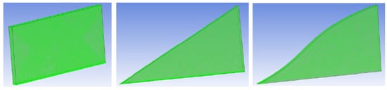
Figure 3.
Schematic diagram of the computational domain (not to scale).
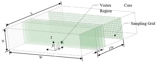
Figure 4.
Rectangular, triangular, and bionic vortex generator shapes and meshes.
The mesh of the computational domain is unstructured, the prismatic mesh is used at the bottom surface, and the height of the first level of the grid is set to 0.0002 to ensure Y+ ≈ 1. Figure 4 shows the mesh of the vortex generator with different shapes, and the grid is encrypted in the flow direction during the grid generation.
After the vortex generator position, a total of 15 detection surfaces are set up at intervals h along the fluid flow direction. The fluid parameters on the detection surface sampling grid are obtained by the post-processing software CFD-POST, as shown in Figure 3.
3.2. The Size of the Vortex
Figure 5 illustrates the radius of the vortex generated by each type of vortex generator for different mounting angles at a 90% confidence level under the flat plate experimental conditions. As the vortex develops along the flow direction, the vortex radius gradually increases, and the larger the mounting angle, the more obvious the increasing trend. The vortex generator’s installation angle has a direct impact on the size of the vortex. When there is a small installation angle (10°), different shapes of the vortex generator and the difference in the size of the vortices are not significant; as the installation angle increases, the vortex size difference increases. The vortex generated by the rectangular vortex generator at different installation angles has the same development characteristics: a fast development region (0,4δ), stable development region (4δ,12δ) and fast dissipation region (12δ,∞).
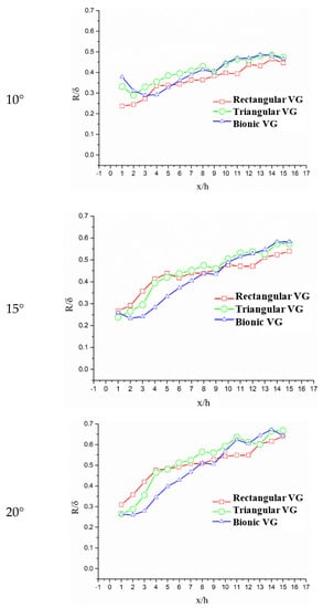
Figure 5.
Vortex radius determined at a 0.9 confidence level.
The process of calculating the vortex intensity by the confidence interval method is as follows: first, the vortex radius is calculated by the confidence interval method, and then the contour of the fitted value of the Gaussian distribution corresponding to the vortex radius is calculated. The vortex strength is then calculated from the region of the contour envelope, and the results are shown in Figure 6. Due to the viscous effect, the vortex intensity has a tendency to decrease gradually. The maximum volume of the ring appears at 2 h after the vortex generator, a phenomenon that can be explained by the fact that the vortex is not fully developed before this position. Although the difference in vortex intensity between the shapes of the vortex generators is not significant, the rectangular vortex generator generates slightly higher vortex intensity than the other shapes as the mounting angle increases. This also validates the conclusion that the vortex intensity is proportional to the vortex generator area in the BAY model.
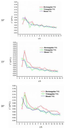
Figure 6.
Vortex strength variation at a 0.9 confidence level.
3.3. The Harmonic Intensity Factor
Figure 7 illustrates the reconciliation strength factor s of the vortex generators with different installation angles. The harmonic intensity coefficients reach the extreme value at 1 h after the vortex generator and decrease gradually along the flow direction; the difference of harmonic intensity coefficients of the different shapes of vortex generators after 6 h is very small, which indicates that the difference of harmonic intensity coefficients caused by shape factors becomes smaller with the gradual dissipation of vortex kinetic energy and the gradual increase in the vortex center. Figure 7 illustrates that the harmonic intensity coefficient of the triangular vortex generator on the 1 h detection surface is significantly higher than the others, which is due to the fact that the vortex core generated by the triangular vortex generator is closer to the wall on the 1 h detection surface.
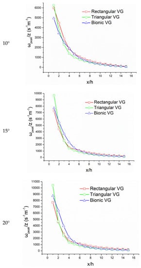
Figure 7.
Variation of the reconciliation strength factor on different testing surfaces.
Based on Figure 7, the reconciliation strength factors of each profile vortex generator are increased with an increasing installation angle, showing the stronger harmonic capability of large installation angle vortex generators for fluids in the boundary layer. This conclusion can also be obtained from Table 1. Table 1 shows the integration of the reconciliation strength factors against the transverse coordinate for different shapes of vortex generators at different mounting angles. It is evident that the rectangular vortex generator is the least sensitive to changes in mounting angle. The integration of the harmonic intensity coefficient of the triangular vortex generator undergoes a process of increasing and then decreasing with an increasing installation angle. The integration of the reconciliation strength factor of the bionic shape vortex generator increases with the increase in the installation angle. Whether the triangular and bionic vortex generators produce extreme values during the increase in the mounting angle needs further investigation. The installation angle is greater than 15°, and the bionic vortex generator is significantly better than the others in terms of the harmonic strength of the fluid in the boundary layer.

Table 1.
Table of the integration values of the harmonic intensity coefficients on the coordinate axes.
3.4. Formatting of Mathematical Components
Godard [9] experimentally compared the performance of rectangular vortex generators and triangular vortex generators for boundary layer control. This paper focuses attention on the performance differences between the bionic vortex generator and the triangular vortex generator, both of which have an installation angle of 15°. The arrangement of the vortex generator is given by Velte [13].
The simulation validation model is adopted from the triangular vortex generator model introduced in the literature [19]. The blade cross-section is a DU97-W-300 wind power airfoil with a span of 0.14 m, a chord length of 0.6 m, a vortex generator height-to-length ratio of 0.294, and an installation angle of 16.4° that is arranged at 0.2c from the leading edge of the blade. The Reynolds number is . ICEM software was adopted for structural meshing, and blocks were created in the first 5 h, last 10 h, and upper 5 h of the vortex generators for an encryption operation. The vortex generators’ spreading direction is divided by the Y-grid, and the grid near the vortex generators is shown in Figure 8. Simulations are performed using ANSYS CFX. As for the boundary conditions, the velocity inlet boundary condition and pressure outlet boundary condition are adopted. Slip-free wall boundary conditions are adopted for the blade section and the vortex generators. The SST two-equation turbulence model is used for the simulation. Since the SST model will overestimate the effect of lift when the angle of attack is large, high lift modification needs to be set to weaken this effect. The comparison of the simulation results of the blade lift coefficient with the experimental results is shown in Figure 9, and the blade section’s pole curve is shown in Figure 10.
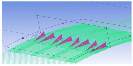
Figure 8.
Schematic diagram of the grid near the vortex generators.
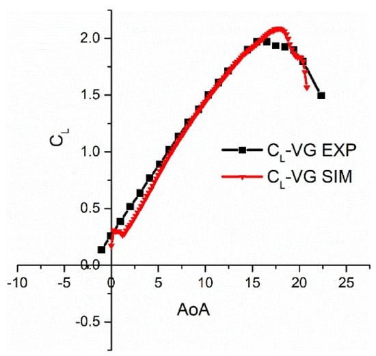
Figure 9.
Comparison between the simulation results and experimental results of the lift coefficient.
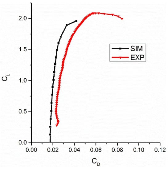
Figure 10.
Comparison between the simulation results and experimental results of the polar curve.
From Figure 9 and pole Figure 10, the simulation results for the lift coefficient basically match the experimental values; however, the simulation results for the drag coefficient are relatively large, causing the pole curve to be shifted to the positive side.
Under the arrangement given in document [13], the vortex generator is mounted at an angle of 15°, with a height of h = 4.5 mm and a center spacing of 5 h, at a distance of 0.2c from the leading edge. The lift coefficients and pole curves of the blade segments for the bionic vortex generators and triangular vortex generators given in this paper are illustrated in Figure 11 and Figure 12. The maximum lift coefficient of the bionic vortex generators is increased by 4.4% compared to the triangular vortex generators. The polar curves of the blade with the two vortex generator profiles are not significantly different when the angle of attack is less than 12°. After the angle of attack is greater than 12°, the blade equipped with the bionic vortex generators shows excellent drag lift performance. This demonstrates that the bionic vortex generator not only enhances the lift coefficient of the blade; this also shows that the drag punishment caused by the installation of the vortex generators is comparatively small. Figure 12 illustrates that the larger the angle of attack, the more pronounced the aerodynamic performance improvement of the blade by the vortex generators. This is because, in a small angle of attack, the boundary layer on the blade does not separate or separation is not significant, and the influence of the vortex generators on the control of the boundary layer is not noticeable. When the angle of attack increases, the boundary layer on the blade is significant, and the vortex generator on the boundary layer control effect will be noticeable.
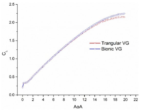
Figure 11.
Blade lift coefficient of vortex generators with different shapes.
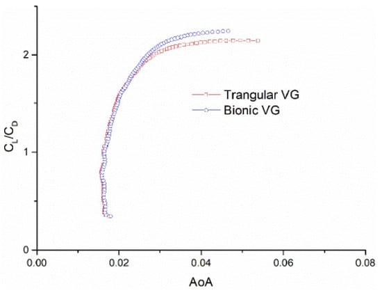
Figure 12.
Blade pole curves of vortex generators with different shapes.
Since the fluid flow status on the blade segment is not the same as that on the plane, the effect of the vortex generators on the lift coefficient’s enhancement does not strictly obey the ratio in Table 1. However, since the control effect of the vortex generators on the boundary layer’s separation is still achieved by mixing the fluid energy within the boundary layer, the order of the strong and weak performance of the vortex generators on the boundary layer’s control of the blade section obeys the order in Table 1, i.e., the bionic shape vortex generators are stronger than the triangular vortex generators. The proposed harmonic intensity factor provides an idea for the evaluation of the vortex generator’s performance through flat plate experiments. With this method, it is possible to avoid the difficulty of meshing and the huge computational effort associated with the way of evaluation accompanied by the lift coefficient of blades.
4. Conclusions
As a passive boundary layer control device that requires no external energy and has no impact on the structure, the vortex generators have a wide range of applications for aerospace and wind turbine efficiency increases. This article improves the calculation method of the vortex radius by introducing the theory of the confidence interval and proposing a performance evaluation criterion of an equal height vortex generator based on Biot–Savart’s theorem. The simulation results demonstrate that the performance of the vortex generator can be effectively evaluated by this evaluation labeling.
The main purpose of this paper was to calculate the vortex strength using the confidence interval and contour method by using the property of the vorticity excited by the vortex generators obeying the Gaussian distribution. The method maximally excludes the randomness of the sample values of the simulation results and the arbitrariness of determining the vortex radius. The vortex size and vortex dissipation process are closer to the real values. The boundary layer problem of flat plate flow around the boundary layer is one of the more intensively understood fluid mechanics problems at present. Since the boundary layer of the flat plate is not affected by noise vortices, the effect of vortex generators on the boundary layer’s control is more easily traced. However, the current research on the vortex generators installed on flat plates is mostly focused on the strength of the vorticity excitation, trajectory, and other aspects, which do not fully capture the control performance of the vortex generators on the boundary layer. Based on this, this paper derives the performance evaluation criterion of the vortex generators on flat plates based on the Biot–Savart theorem, i.e., the harmonic intensity factor . The simulation results show the positive correlation between this coefficient and the evaluation results with the assistance of the lift coefficient. Harmonic strength factor is proposed to facilitate the direct evaluation of the performance of vortex generators by scholars, which can avoid the increased difficulty and time-consuming evaluation of the methods of the accompanying intermediate variables.
Author Contributions
Conceptualization, Z.Z. and W.L.; The remainder of the work was completed by W.L. All authors have read and agreed to the published version of the manuscript.
Funding
This research was supported by the Fundamental Research Funds for the Central Universities, grant number 2019QN021.
Conflicts of Interest
The authors declare no conflict of interest.
References
- Lin, J.C. Review of research on low-profile vortex generators to control boundary-layer separation. Prog. Aerosp. Sci. 2002, 38, 389–420. [Google Scholar] [CrossRef]
- Gad-el-Hak, M.; Bushnell, D.M. Separation control: Review. J. Fluids Eng. 1991, 113, 5–30. [Google Scholar] [CrossRef]
- Taylor, H.D. The Elimination of Diffuser Separation by Vortex Generators; United Aircraft Corp: Chicago, IL, USA, 1947. [Google Scholar]
- Titchener, N.; Babinsky, H. A review of the use of vortex generators for mitigating shock-induced separation. Shock Waves 2015, 25, 473–494. [Google Scholar] [CrossRef] [Green Version]
- Dai, L.P.; Jiao, J.D.; Li, X.K.; Kang, S.; Zhao, P. Numerical Investigation on Effect of Installation Position of Vortex Generator on Aerodynamic Characterisitics of Wind Turbine Airfoil. Acta Energ. Sol. Sin. 2016, 37, 276–281. [Google Scholar]
- Squire, H.B. The Growth of a Vortex in Turbulent Flow. Aeronaut. Q. 1965, 16, 302–306. [Google Scholar] [CrossRef]
- Urkiola, A.; Fernandez-Gamiz, U.; Errasti, I.; Zulueta, E. Computational characterization of the vortex generated by a Vortex Generator on a flat plate for different vane angles. Aerosp. Sci. Technol. 2017, 65, 18–25. [Google Scholar] [CrossRef]
- Fernandez, U.; Réthoré, P.E.; Sørensen, N.N.; Velte, C.M.; Zahle, F.; Egusquiza, E. Comparison of Four Different Models of Vortex Generators; European Wind Energy Conference & Exhibition European Wind Energy Association: Copenhagen, Denmark, 2012; pp. 1–13. [Google Scholar]
- Godard, G.; Stanislas, M. Control of a Decelerating BoundaryLayer, Part 1: Optimization of Passive Vortex Generators. Aerosp. Sci. Technol. 2006, 10, 181–191. [Google Scholar] [CrossRef]
- Martínez-filgueira, P.; Fernandez-gamiz, U.; Zulueta, E.; Errasti, I.; Fernandez-Gauna, B. Parametric study of low-profile vortex generators. Int. J. Hydrogen Energy 2017, 42, 17700–17712. [Google Scholar] [CrossRef]
- Velte, C.M. Vortex generator flow model based on self-similarity. AIAA J. 2013, 51, 526–529. [Google Scholar] [CrossRef] [Green Version]
- Gao, L.Y.; Zhang, H.; Liu, Y.Q.; Han, S. Effects of vortex generators on a blunt trailing-edge airfoil for wind turbines. Renew. Energy 2015, 76, 303–311. [Google Scholar] [CrossRef]
- Velte, C.M.; Hansen, M.O.L.; Meyer, K.E.; Fuglsang, P. Evaluation of the Performance of Vortex Generators on the DU 91-W2-250 Profile Using Stereoscopic PIV. In Proceedings of the 12th World Multi-Conference on Systemics, Cybernetics and Informatics, Orlando, FL, USA, 1 January 2008; pp. 263–267. [Google Scholar]
- Skrzypinski, W.; Gaunaa, M.; Bak, C.; Junker, B.; Brønnum, N.B.; Kruse, E.K. Increase in the annual energy production due to a retrofit of vortex generators on blades. Wind Energy 2020, 2020, 617–626. [Google Scholar] [CrossRef]
- Bray, T.P. A Parametric Study of Vane and Air-Jet Vortex Generators; College of Aeronautics: Metro Manila, Philippines, 1997. [Google Scholar]
- Ruben, G.A.; Unai, F.G.; Iñigo, E.; Zulueta, E. Computational Modelling of Three Different Sub-Boundary Layer Vortex Generators on a Flat Plate. Energies 2018, 11, 3107. [Google Scholar] [CrossRef] [Green Version]
- Lin, J.Z.; Ruan, X.D.; Chen, B.G.; Wang, J.P.; Zhou, J.; Ren, A.L. Fluid Mechanics, 2nd ed.; Tsinghua University Press: Beijing, China, 2013; pp. 190–194. [Google Scholar]
- Zhang, Z.H.; Li, W.W.; Jia, X.N. CFD Investigation of a Mobula Birostris-Based Bionic Vortex Generator on Mitigating the Influence of Surface Roughness Sensitivity of a Wind Turbine Airfoil. IEEE Access 2020, 8, 1. [Google Scholar] [CrossRef]
- Timmer, W.A.; Van Rooij, R.P.J.O.M. Summary of the Delft University Wind Turbine Dedicated Airfoils. J. Sol. Energy Eng. 2003, 125, 488–496. [Google Scholar] [CrossRef]
Publisher’s Note: MDPI stays neutral with regard to jurisdictional claims in published maps and institutional affiliations. |
© 2022 by the authors. Licensee MDPI, Basel, Switzerland. This article is an open access article distributed under the terms and conditions of the Creative Commons Attribution (CC BY) license (https://creativecommons.org/licenses/by/4.0/).