Energy Efficiency Increase Achieved by Dedicated Rule-Based Control of Chillers Operating in the Data Center

Abstract

Commercial solutions in the area of data center cooling available on the market are universal solutions that use dedicated control methods and are to able function properly in a wide range of working conditions. The functional limitations resulting in their application were our motivation for developing our own system architecture and a dedicated control algorithm. Historical data from an operating cooling system were analyzed. On that basis, a rule-based controller was developed, the purpose of which is to correctly switch between operating modes. The time constants of the automation actuators and the dynamics of the changes that occur in the cooling process were identified. The control strategy was experimentally validated throughout 2017. The efficacy of the second solution and the effectiveness of the control algorithm throughout the calendar year were demonstrated. Our solution allows individual control of each element of the cooling system. This enabled the extension of the operation time in the free-cooling mode by 2064 h throughout the year, a 69% increase in the COP coefficient of the cooling system and a reduction in electricity consumption by 206.9 MWh due to longer operation in the freecooling mode.

1. Introduction

On the basis of research and analysis of a cooling system’s operation in the POLCOM data center in 2015 [1], its advantages and disadvantages, along with possibilities for optimization, modernization and development were identified. Based on the analyses carried out, it was decided to modernize the system. The work began in 2016 and ended in 2017. The modernized cooling system reached full capacity in 2017. The modernization of the cooling system was aimed at improving its operating parameters and energy efficiency. As the cooling system is the most energy-consuming part of a technical data center [2,3,4], improving its efficiency would significantly reduce the operating costs of the data center [5,6]. Based on the results of the analysis of the system in 2015, the objectives of the modernization were to extend the operating time and cooling capacity in freecooling mode (FC), which is more effective than compressor mode (CP) [7,8,9,10]. It was also important to be able to achieve full control over the switching moment of the system between CP and FC modes [11]. A dedicated control system for chillers allows for significant savings in electricity consumption, not only in data center buildings but also in office buildings and plants [12,13,14]. The modernization in question consisted of two parts: hardware and software. The equipment part concerned the installation of modern, highly efficient chillers with centrifugal compressors based on magnetic levitation technology and high performance drycoolers. The software part was based on the design and implementation of an original, dedicated system for controlling the process of cooling energy production.

Note that active magnetic bearings [15,16,17] are regarded as the best solution for compressors [18,19,20] because of their advantages: no mechanical contact, control of rotor dynamics, complete state monitoring, variable speed and control of dynamical properties. Friction is reduced because they operate without the use of oil for lubrication. Thus, the evaporator or condenser operates in a clean environment, and therefore, heat transfer efficiency increases [21]. Variable speed control is used to guarantee appropriate performance [22], and the magnetic bearing controllers guarantee robustness over a wide range of rotational speeds [20]. It is well known that variable-speed magnetic bearing chillers operate most efficiently well below their full load. Therefore, it is a necessity to optimize the cooling system they are in [21]. Chillers are composed of multiple compressors with magnetic bearing technology, which guarantees redundancy and functional diversity. They can attain optimum efficiency while operating under partial loads [23]. Typically, compressors work in a conservative way to guarantee stability and preserve surge effects. When applied, surge control can be realized in the case of a compressor with a levitating rotor. The axial AMB can be applied to adjust the tip clearance between impeller tip and the static shroud of a compressor to achieve surge control [24]. It could be realized with high bandwidth and precision [19]. Therefore, we expected that a chiller with magnetic levitation technology would improve the performance of the cooling system.

This paper is organized in the following way: Section 2 describes briefly the configuration of cooling systems and operating modes. In Section 3, the custom control strategy for switching between two modes is given and illustrated with histograms. Discussion on BREF and Turbocor systems is initiated. The detailed analysis of a few cases under the proposed control strategy is presented in Section 4. The COP coefficient is analyzed in Section 5. Section 6 shows two critical situations and the behavior of the cooling system under control. Throughout this publication we present material that responds to the following questions: What changes in the energy efficiency ratio does the cooling system modernization produce? What does the operating profile of the cooling system look like under different temperature conditions? What benefits are achieved by using a control algorithm superior to direct control by the chiller controllers? What were the differences in the operation and capacity of the cooling system before and after the modernization? How does the cooling system respond when the supply voltage drops?

2. Configuration of the Cooling System

2.1. Components of the Cooling System

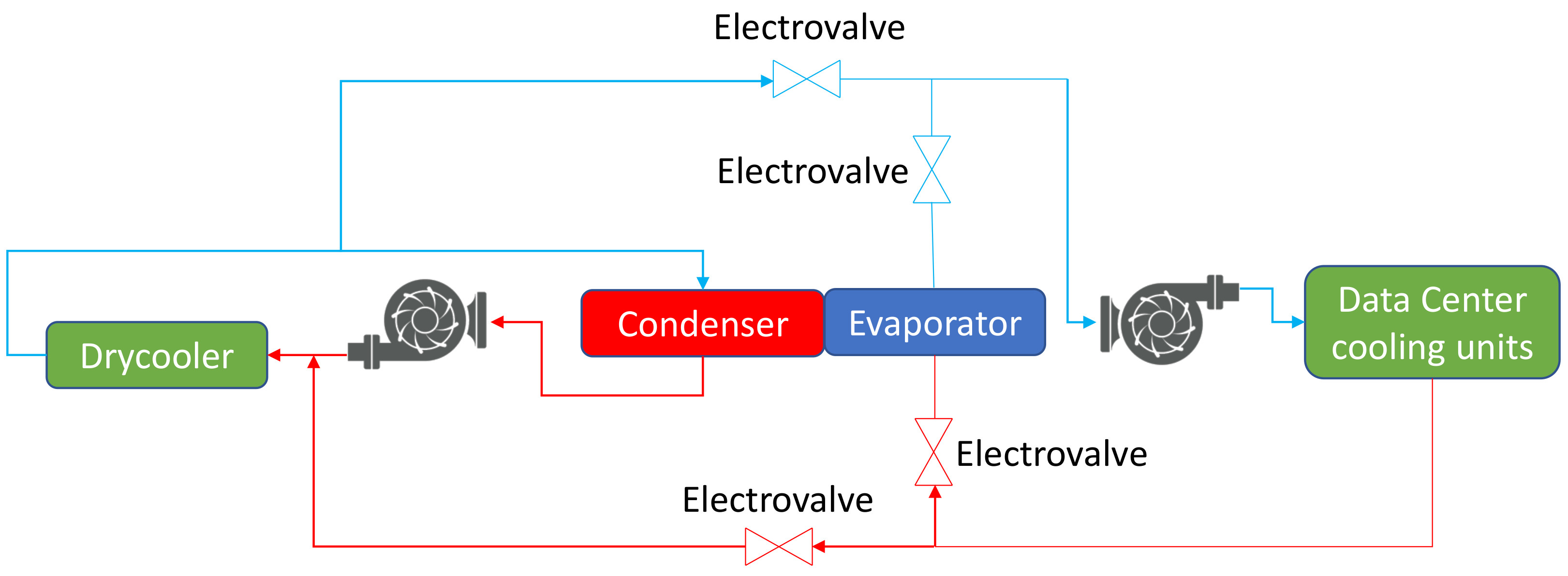
The modernization of cooling systems has changed our approach to units that produce coldness. Originally, the cooling system in question used monolithic external chillers equipped with screw compressors (in the POLCOM company nomenclature marked as BREF units). These units consisted of the following components: compressors, refrigerant system exchangers, circulation pumps, chilled water coolers and an automatic system that switches the modes of operation of the chiller. The disadvantage of such a system was the inability of the user to control individual components of the chiller.

We proposed to separate the components of the chiller into autonomous units. For this purpose, an internal unit with Danfoss Turbocor oil-free centrifugal compressors [22] was used without air exchangers, with circulation pumps and with automatic switching between operating modes. As a liquid–air exchanger, a 12-fan drycooler with “V” system coolers was used. The circulation pumps controlled by inverters were selected, and the piping was equipped with controlled electrovalves. A proprietary algorithm was developed and implemented to manage the work (cooperation) of individual components of the cooling system, in particular, the switching between modes of operation.

After the modernization, two existing external chillers with screw compressors and two internal Turbocor units with centrifugal compressors operated in parallel (see Figure 1).

The technical parameters of the chiller in nominal operating conditions are shown in

Table 1. Technical parameters of the chiller.

Chiller	Cooling Capacity	Absporbed Power	COP
BREF	477 kW	149 kW	3.12
Turbocor	630 kW	134 kW	4.71

. The nominal operating conditions for BREF chillers are: evaporator in/out temperature 12 ${}^{°}$C/7 ${}^{°}$C and condenser in/out temperature 30 ${}^{°}$C/35 ${}^{°}$C. The nominal operating conditions for Turbocor chillers are: evaporator in/out temperature 12 ${}^{°}$C/7 ${}^{°}$C and external temperature 35 ${}^{°}$C.

The modernization of the cooling system concerned only the cold sources (chillers, drycooler and pumps). The elements of the cooling system in the server room (precision air-conditioning cabinets) did not change. For this reason, the data presented in this publication concern only modernized cooling sources. The power consumption of the cooling system does not include the power consumed by the precision air conditioning cabinets. Thus, the COP is determined only for the cooling sources.

2.2. Specificity of the Operation of Turbocor Internal Chillers

Turbocor units with centrifugal compressors are internal water–water units. They are equipped only with refrigerant circuit elements (compressors, evaporator, condenser), together with the controller, sensors and instrumentation. They do not participate in the FC operation of the cooling system (they are switched off). They operate only in compressor mode; they cool the water flowing through the evaporator and transfer heat to the water flowing through the condenser. The water is then transported by piping to the drycooler, where it is returned to the environment.

2.3. Specificity of the Operation of the Drycooler

The drycooler is an external water–air heat exchanger, which transfers heat from the water flowing through it to the surrounding air, whose movement is forced by fans, and it works in both FC and CP modes. In freecooling mode, it cools the hot water returning from air conditioning cabinets, and in compressor mode, it cools the hot water from the condenser of the Turbocor unit.

2.4. Process Data Acquisition System

The cooling system was equipped with sensors and measuring devices, the use of which allowed for continuous data recording throughout 2017.

A HOTCOLD HCRH-Modbus sensor was used to measure the outside temperature. The cooling capacity of chillers was measured using ENKO MPP6 electromagnetic flow meters and HOTCOLD HC511 temperature sensors. SOCOMEC E44 energy meters were used to measure the electric power. The PLC controller was collecting signals from the sensors. The data were then sent to a database for archiving. The data collected throughout the year is a recording of unique operating conditions system.

For all analyses, with the exception of Section 6, the data recorded at 5-min intervals were used. The analysis of the system’s response to the supply voltage drop, due to the high dynamics of change, required the use of 10-s resolution data.

The developed dedicated control strategy, described at the beginning of Section 3, was tested in a commercially operating server room throughout 2017. The rest of Section 3 focuses on the analysis of the cooling system operating time in individual operating modes. Section 3 also describes the behavior of the refrigeration system in an emergency. Section 4 provides a detailed annual analysis of the cooling system in terms of the cooling capacity produced and electrical power consumed. Section 5 contains the COP analysis, and Section 6 of the part presents and analyzes interesting situations that took place during the operation of the refrigeration system with a dedicated control strategy during operation in 2017.

3. Control System and Strategy

The inability to select and control the switching point of the BREF system between operating modes was one of the major operational concerns. When designing a new system based on Turbocor units, it was assumed that it should be possible to directly select the switching point by means of the control algorithm.

Therefore, a unique system for controlling the elements of the cooling system was proposed, which would improve its efficiency.

The triggering condition for the switching procedure was to exceed specific thresholds (values) of the outside temperature. These values were determined experimentally on the basis of previous observations of the capacity of the cooling system [1] and modified throughout the year as required. The switching procedure is based on the relay with hysteresis in line with the following formula:

$$u\left(t\right)=\left\{\begin{array}{c}0,T_{ext}\left(t\right)\ge T_s\hfill \\ u_s,T_s-T_h<T_{ext}\left(t\right)<T_s\hfill \\ 1,T_{ext}\left(t\right)\le T_s-T_h\hfill \end{array}\right.$$

(1)

where: $T_{ext}$—outside temperature; $T_s$ = 12 ${}^{°}$C—threshold temperature for switching between operating modes; $T_h$ = 1.5 ${}^{°}$C—switching hysteresis between operating modes; $u_s$ is either 0 or 1 depending on the current state of the FSM.

The controller gives two state outputs $\left\{0\right\},\left\{1\right\}$ that correspond to CP and FC modes, respectively. When the control system is in the CP mode (state $Q4$) and the external temperature is decreasing towards $T_s-T_h$, then $u_s$ stays in CP mode. If the control system is in the FC mode (state $Q8$) and external temperature is increasing towards $T_s$, the $u_s$ keeps the FC mode.

During this procedure, the master automation system controls such elements of the system as: a chiller, a drycooler, circulation pump inverters and valve actuators.

In the control system the following binary inputs are defined:

• $x_1\in \{0,1\}$—status of circulation pumps: 1—in operation, 0—stopped;
• $x_2\in \{0,1\}$—status of freecooling valves: 1—open, 0—closed;
• $x_3\in \{0,1\}$—status of evaporator valves: 1—open, 0—closed;
• $x_4\in \{0,1\}$—status of fluid flow through evaporator and condenser: 1—flow present, 0—no flow;
• $x_5\in \{0,1\}$—status of turbocor operating mode: 1—operating, 0—stopped.

The output signals that control particular devices are set in a form of binary outputs.

• $y_1\in \{0,1\}$—signal to circulation pumps inverters: 1—start, 0—stop;
• $y_2\in \{0,1\}$—control of freecooling valves: 1—open, 0—close;
• $y_3\in \{0,1\}$—control of evaporator valves: 1—open, 0—close;
• $y_4\in \{0,1\}$—selection of drycooler setpoint for appropriate mode: 1—compressor, 0—freecoling;
• $y_5\in \{0,1\}$—control of turbocor unit: 1—start, 0—stop.

Initally, the system is in a state $Q0$ and starts with an initialization procedure.

While operating, the system remains in two stable states $Q4$ and $Q8$, which guarantee CP and FC operation modes, respectively. Outputs are modified in a dedicated sequence to ensure that the cooling system works effectively.

This control strategy is based on the main rule that the subsequent stage must be acknowledged by the correct realization of the preceding step. Corresponding inputs are analyzed and the transition between states can be executed. Therefore, a few states form $Q1$ to $Q3$ and from $Q5$ to $Q7$ can be defined in the control sequence between stable operating modes. The graphical representation of the finite state machine is presented in Figure 2. Here is a complete list of states with outputs being set at the state entry:

• Q1—initialization after system start-up that configures outputs: $y_1=1$, $y_2=0$, $y_3=1$, $y_4=1$, $y_5=1$, starting the transition towards compressor mode: $Q_1$, $Q_2$, $Q_3$, $Q_4$;
• Q1: set $y_1=0$;
• Q2: set $y_2=0$, $y_3=1$;
• Q3: set $y_1=1$;
• Q4—stable state realizing control in compressor mode;
• Q5: set $y_5=0$;
• Q6: set $y_1=0$;
• Q7: set $y_2=1$, $y_3=0$;
• Q8—stable state realizing control in freecooling mode.

The defined sub-states are necessary to achieve robustness of the control system. Even when the same failure occurs, it is very easy to diagnose the system state due to the well-defined procedure. The permanent monitoring of the data center by the qualified staff allows for a quick response to any malfunction. The rules describing the switching control from CP to FC state can be formulated as follows:

• Being at $Q4$, start procedure to switch towards FC mode: if $T_{ext}$ < $T_s-T_h$, then go to $Q5$;
• Being at $Q5$, wait until Turbocor chiller stops: if $x_5$ is 0, then go to $Q6$;
• Being at $Q6$, wait until pumps stop: if $x_1$ is 0, then, go to $Q7$;
• Being at $Q7$, wait until freecooling valves open and evaporator valves close: if ($x_2$ is 1) AND ($x_3$ is 0), then go to $Q8$;
• Being at $Q8$, start procedure to switch towards CP mode: if $T_{ext}$ ≥ $T_s$, then go to $Q1$;
• Being at $Q1$, wait until circulation pumps stop: if $x_1$ is 0, then go to $Q2$;
• Being at $Q2$, wait until freecooling valves close and evaporator valves open: if ($x_2$ is 0) AND ($x_3$ is 1), then go to $Q3$;
• Being at $Q3$, wait until fluid flow is present: if $x_4$ is 1, then, go to $Q4$.

The every state transition and realization is monitored by the supervisory watchdog algorithm where the maximal execution time is specified. In the case of any delay, the supervisory operator maintaining the system 24 h per day is alarmed.

The implementation of the proposed algorithm at the simulation stage allowed a set of complex tests to be performed (see Figure 3). The input/output signals were used to emulate the real actuators. The outdoor temperature profiles were chosen from the experimental data set for particular climate conditions. This approach allowed switching modes to be tested. Detailed time diagrams present the simulation of control strategy. Moreover, the implementation of the control scenario in the form of a state flow diagram and the ability to slow down the execution of the simulation made it possible to track transitions between set and active states during execution.

3.1. Operation Modes in Cooling System

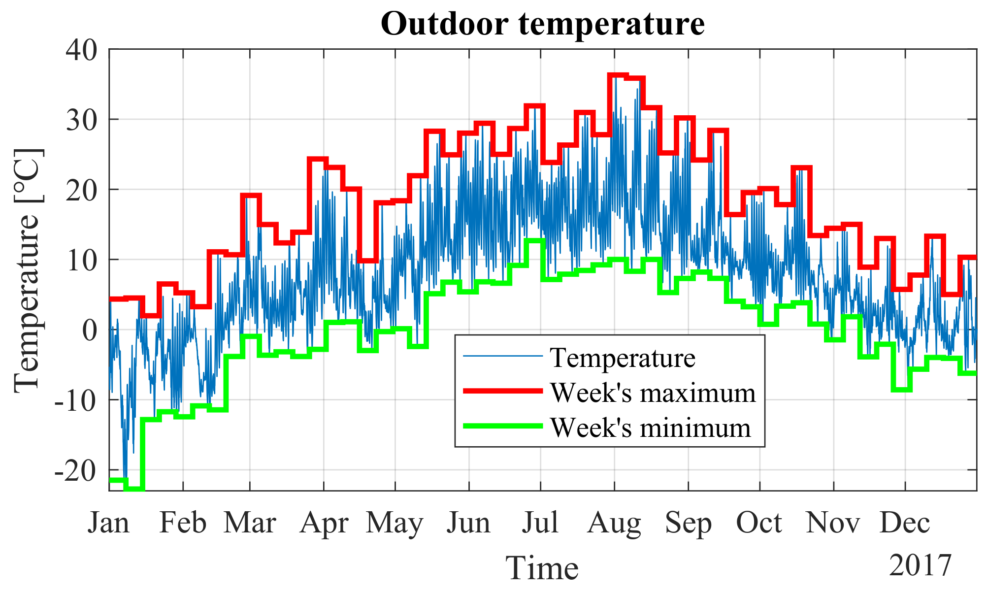
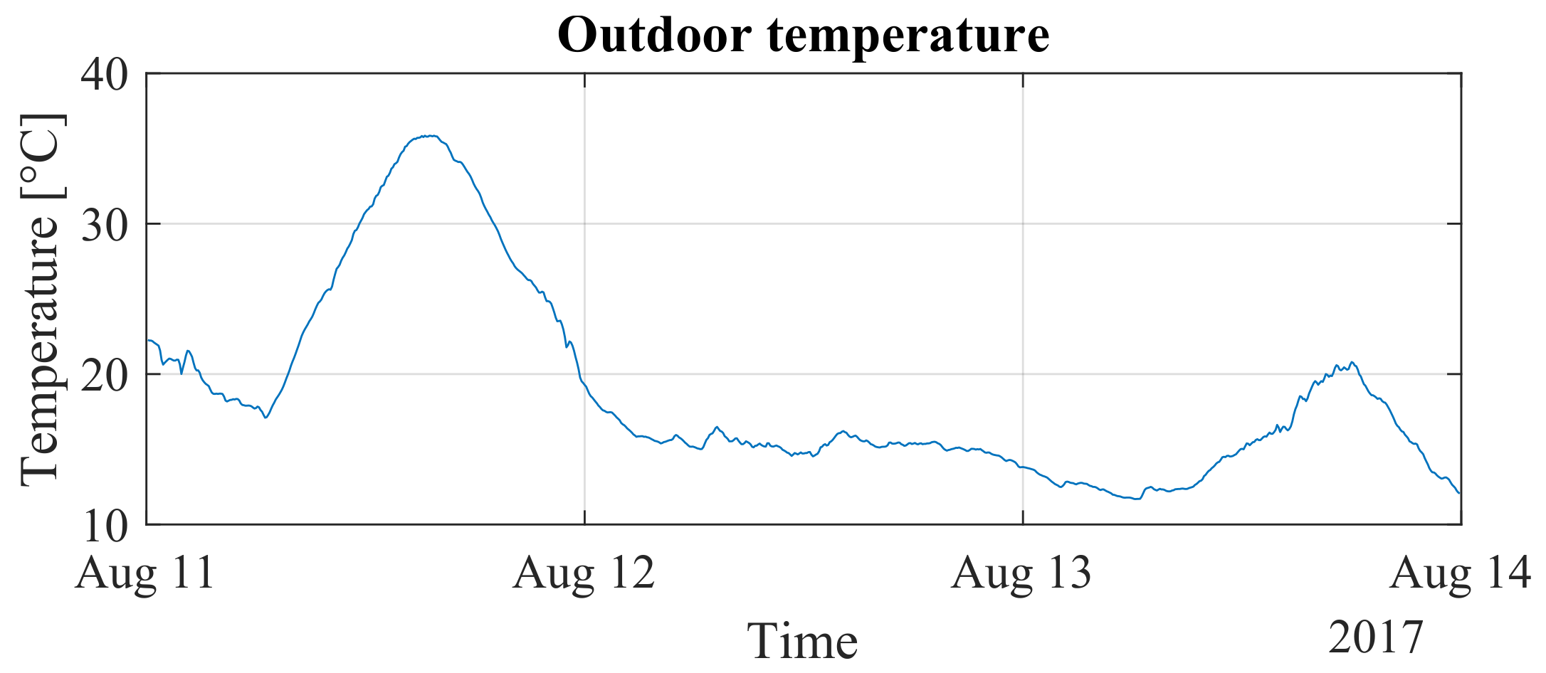
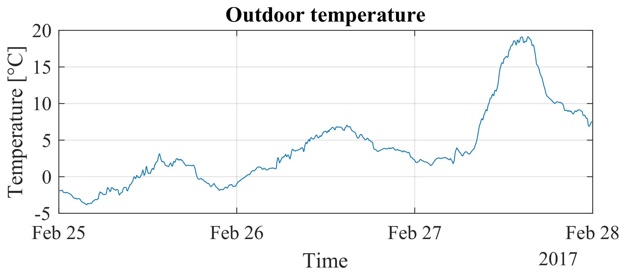
The main objective of the modernization of the data center cooling system was to increase the operating time of the cooling system in FC mode. Based on the analysis of 2015 [1], it was observed that the internal control systems of the chillers determined the operation mode independently of the external control system, under different outdoor conditions, thereby limiting the potential for FC operation. In order to verify that the assumptions were met throughout 2017, the necessary parameters of the cooling system operation were recorded (including the current mode of operation). Thanks to the fact that the cooling system based on BREF outdoor chillers and the new cooling system based on Turbocor indoor chillers operated in parallel throughout the year, it was possible to compare the performances of both systems in the same time frame and under the same climate conditions. Data on the course of the annual temperature are presented in Figure 4.

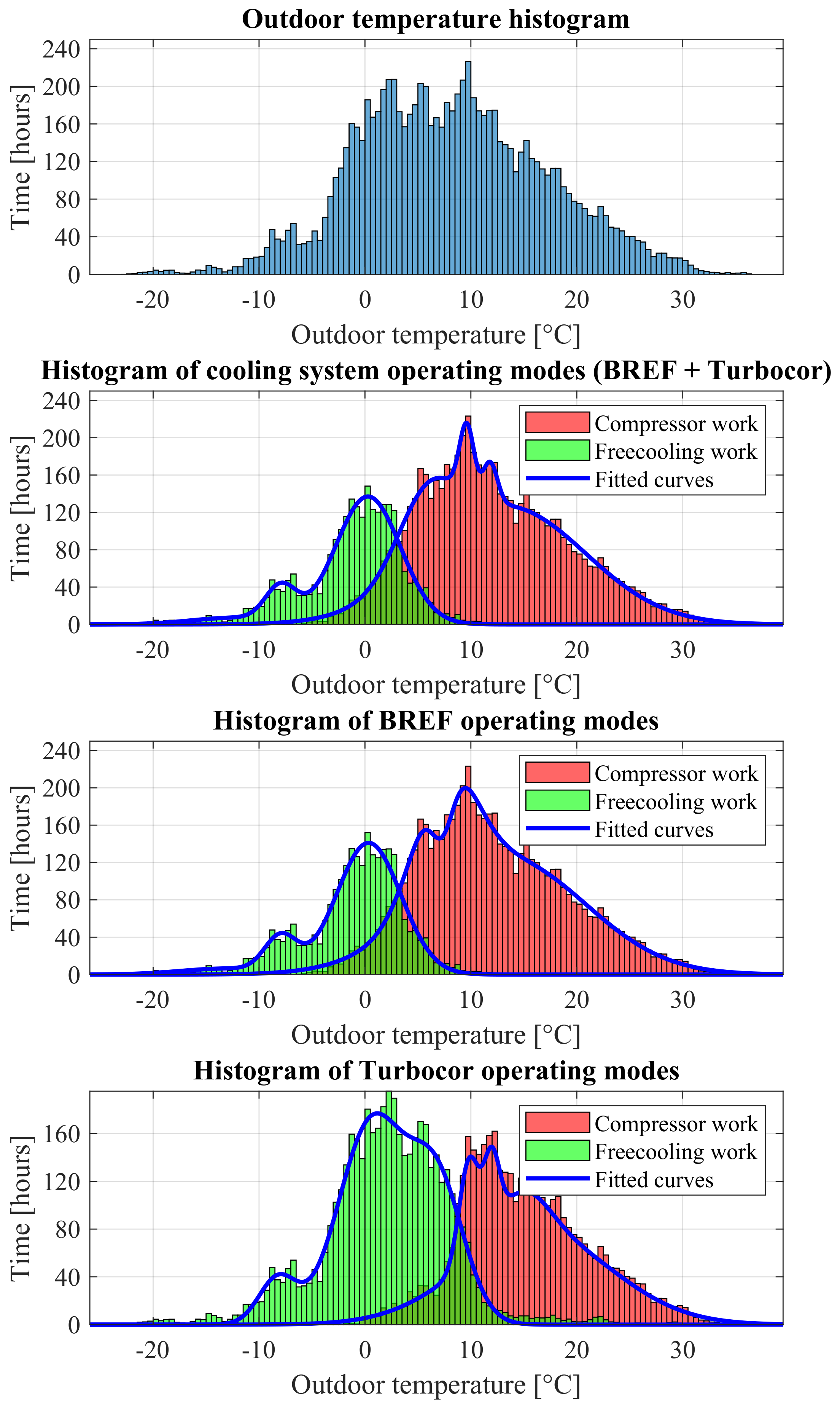
Figure 5 shows the time spent by the cooling systems in both operating modes in relation to the outside temperature. A separate chart is visible for the whole system, for external chillers and for Turbocor chillers.

Two schedules are visible, corresponding to CP mode and FC mode. The FC mode schedule is 0 ${}^{°}$C for the BREF system, 4 ${}^{°}$C for the Turbocor system and 1 ${}^{°}$C for the whole system. The compressor distribution axis is 11 ${}^{°}$C for the BREF system, 13 ${}^{°}$C for the Turbocor system and 12 ${}^{°}$C for the whole system. One can see that the fitted curves correspond to multi-modal distributions. The general form (3) based on Gaussian distribution (2) was optimized for the operating modes (FC and CP) separately.

$$f_{\mu ,\sigma }\left(x\right)=\frac{1}{\sigma \sqrt{2\pi }}exp\left(\frac{-{(x-\mu )}^2}{2{\sigma }^2}\right)$$

(2)

$$f_n\left(x\right)=\sum _{i=1}^n{w}_i{f}_{{\mu }_i,{\sigma }_i}\left(x\right)$$

(3)

The values of coefficients for individual distributions were determined and can be used in further prediction for control purposes.

The $MSE$ of the fitted curves were as follows: for the BREF + Turbocor system in FC mode $MSE$ = 0.9771, for the BREF + Turbocor system in CP mode $MSE$ = 0.9889, for BREF system in FC mode $MSE$ = 0.9770, for theBREF system in compressor mode $MSE$ = 0.9864, for the Turbocor system in FC mode $MSE$ = 0.9824 and for the Turbocor system in CP mode $MSE$ = 0.9895.

The Turbocor system had longer freecooling operation time than the BREF system. The difference in the freecooling operation time for these systems was 2064 h. The operating time of the Turbocor system in FC mode in relation to the operating time of the BREF system in FC mode was therefore increased by 78%. The modernization of the cooling system had a measurable impact on the improvement of the freecooling operation time. Details of working time are shown in

Table 2. Annual operating time of cooling systems, broken down by modes of operation.

System	Freecooling Mode	Compressor Mode
BREF + Turbocor	2587 h (29.5%)	6173 h (70.5%)
BREF	2637 h (30.0%)	6123 h (70.0%)
Turbocor	4701 h (53.7%)	4059 h (46.3%)

.

The Turbocor system operated in FC mode for 4701 h in the year, consuming an average of 22 kW of electricity per hour. This totals 103.4 MWh of electricity consumed. At the same time, the BREF system consumed on average 66 kW of electricity per hour, consuming 310.3 MWh of electricity overall. The modernization of the cooling system together with the control system therefore enabled the generation of annual savings in electricity consumption of 206.9 MWh only by extending the freecooling operation time. Taking into account that the Turbocor system, working in FC mode, generated an average of 456 kW of cooling capacity and the BREF system an average of 386 kW, the specific electricity required to produce 1 MWh of cooling energy for the Turbocor system was 0.05 MWh, but for the BREF system 0.17 MWh. This means an increase in the efficiency of the new cooling system by 340% for outdoor temperatures corresponding to freecooling operation.

3.2. Effects of Location and Ambient Temperature on Operating Modes

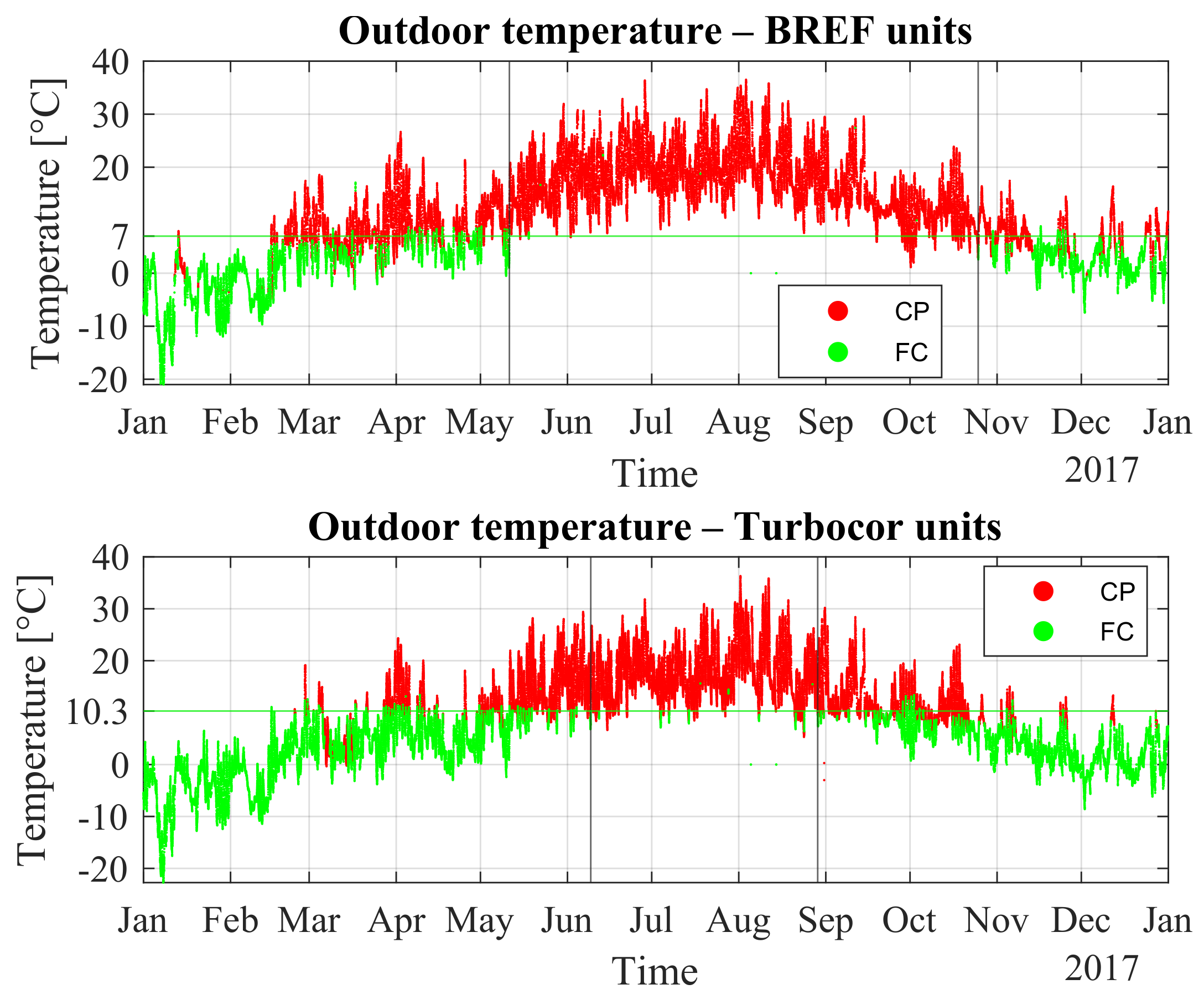
Both the BREF and Turbocor systems worked within one data center building. However, the locations of these systems differed. BREF units were installed on the eastern side of the building and the Turbocor system drycooler on the western side. In addition, the drycooler was shielded from sunlight from the south. The outside temperature was measured in two places. For BREF units, the measuring point was a temperature sensor installed by the BREF units, and for the Turbocor units, a sensor installed near the drycooler. Due to different reading locations, there were differences in the outside temperature values for both Turbocor and BREF systems. The average annual outdoor temperatures were 10.1 and 8.1 ${}^{°}$C for for BREF units and Turbocor units, respectively. The difference in average values resulted from the fact that the BREF units were installed in a place less sheltered from sunlight, compared to the more heavily shielded drycoolers of the Turbocor system.

Figure 6 shows the annual outdoor temperatures for both BREF and Turbocor systems. Separate colors are used for compressor and freecooling modes.

Figure 6 also shows the average annual limit temperature of the system in FC mode (horizontal straight line). For the BREF system it was 7.0 ${}^{°}$C, and for the Turbocor system it was 10.3 ${}^{°}$C. The time interval in which FC mode (over one hour per day) was used is also marked. For the BREF system, the freecooling operation took place until 11 May and from 25 October. For the Turbocor system, the freecooling operation took place from 9 June to 29 August.

In the first half of January, minimum annual temperatures of −22.7 ${}^{°}$C were recorded. At the turn of July and August, temperatures of up to 36.5 ${}^{°}$C were recorded. The annual temperature amplitude was, therefore, 59.2 ${}^{°}$C in 2017. Despite such a high outdoor temperature amplitude, the cooling system was stable.

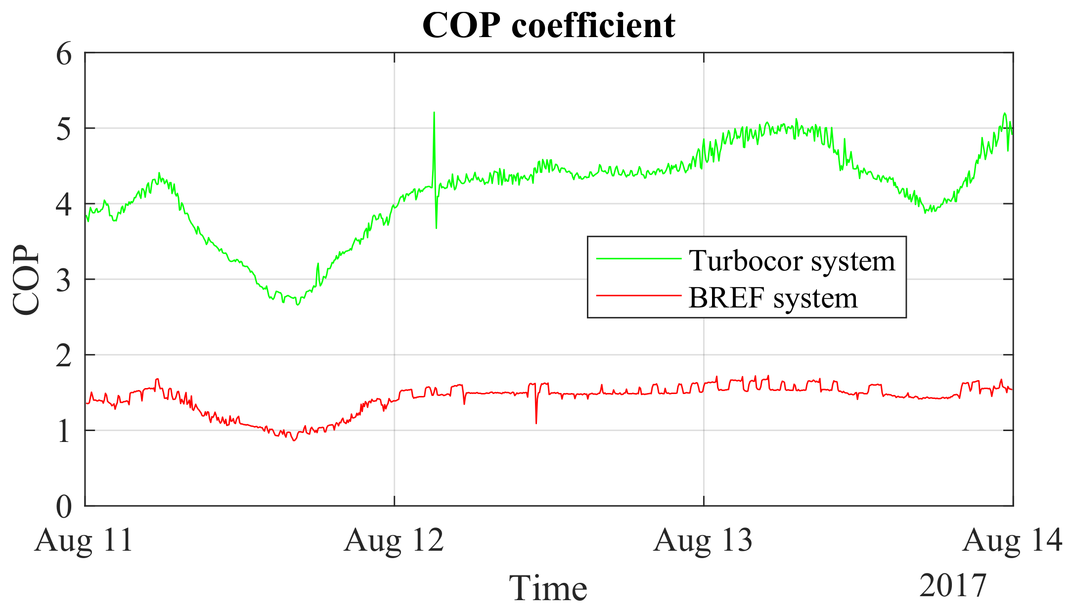
3.3. Robustness of the System to a Momentary Supply Voltage Drop

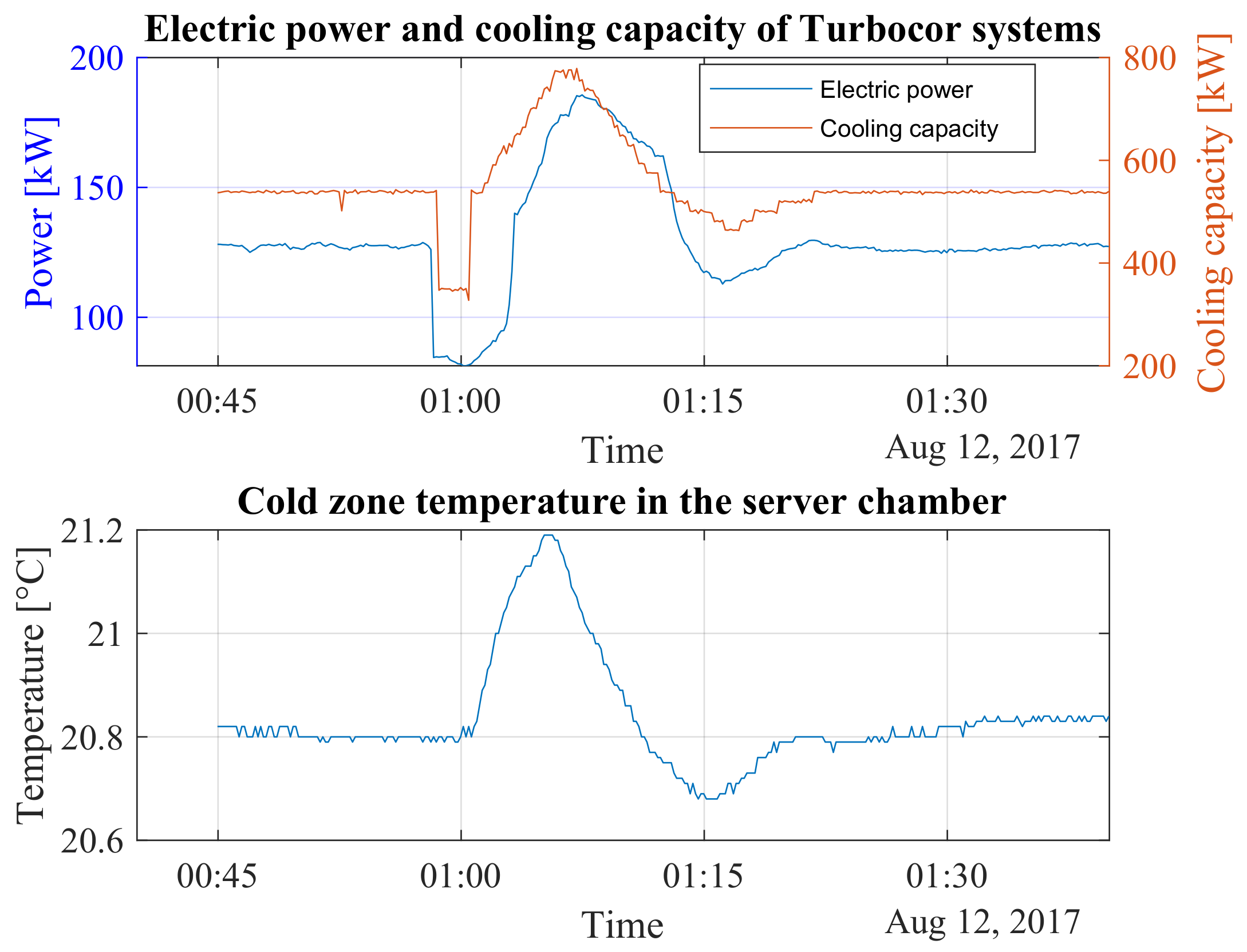
The Turbocor system consists of two compressors. Each of them is powered from a different feeder track. On 12 August 2017, there was a temporary drop in the supply voltage on one of the two lines supplying the facility (the interphase voltage dropped from 393 to 387 V). This drop caused one of the compressors to generate a “Power Failure” alarm and stop. The compressor controller is very sensitive to supply voltage anomalies. The cause of that is the magnetic bearing-based levitation system of the compressor, which in the event of power failure does not perform its function. The compressor must therefore be stopped quickly, enough in the event of a power failure so that the rotor does not become delevitated. For this reason, the controller does not wait for large supply voltage anomalies, but immediately stops the compressor with a 1% anomaly. From the user’s point of view, this is not desirable because it causes interruptions in the supply of cooling power. From the point of view of compressor durability, this is essential for long and trouble-free operation. The compressor is equipped with high capacity capacitors, which, in the event of a sudden and complete power outage, are the source of electrical energy that keep the magnetic bearings running until the compressor rotor stops. The 12 August event became the inspiration for further analyses and work on a fault tolerant control system, the functionality of which will be implemented in the future to control the master cooling system.

The recorded electricity consumption patterns and the cooling capacity generated by the Turbocor system are shown in Figure 7. At 00:58, a power supply voltage drop occurred. As a result of the drop and shutdown of one of the compressors, electric power consumption decreased from 126 to 85 kW. This resulted in a reduction in the value of heat energy given off by the Turbocor unit to the drycooler. As a result, the less loaded drycooler reduced the speed of the fans and thus its own power consumption. This decrease is visible in the chart from 00:59 to 01:00 (from 85 kW to 81 kW). We can then observe a continuous increase in power consumption up to 186 kW. The reason for this increase is the fact that the unit restarted the compressor and tried to stabilize the increased temperature of water output from the chiller, which was raised as a result of a temporary decrease in the level of generated cooling capacity. When the maximum electrical power consumption was reached, the chilled water temperature began to stabilize, to which the chiller controller reacted by reducing the compressor capacity. This resulted in a decrease in power consumption to 113 kW. At 1:16, the first over-regulation of the chiller capacity due to an excessively low chilled water temperature was visible. The chiller did not reduce compressor capacity quickly enough, which resulted in the water cooling and the need to temporarily reduce cooling capacity so that the chilled water temperature rose to the target value. From 1:22, we observed stabilization of electric power consumption and cooling capacity of the chiller at 126 and 540 kW, respectively.

For a more complete analysis of this case, data on the temperature of the chilled water from the Turbocor unit would be helpful. However, such data were not logged in 2017. It was possible to use the data concerning air temperature in the cold zone of the server chamber. The course of this temperature is shown in Figure 7.

The effect of switching off one of the compressors (at 00:58) was an increase in air temperature in the server chamber. The temperature rise in the chamber started at 1:00, 2 min after the compressor was switched off. The reason for this time inertia was the time for chilled water of higher temperature to reach the precision air-conditioning cabinets located in the server chamber and the time during which the precision air-conditioning cabinets were able to compensate for higher chilled water temperatures by opening their control valves, trying to keep their cooling capacity constant. When the control valves of precision air-conditioning cabinets were fully open, it was no longer possible to compensate for the rising chilled water temperature, which in turn led to a temperature rise in the server compartment, from 20.8 to 21.2 ${}^{°}$C. Then from 1:05, we observed a decrease in the temperature in the chamber caused by the supply of chilled water of lower temperature to the cabinets. The temperature drop reached the minimum of 20.7 ${}^{°}$C. This was followed by gradual temperature stabilization. Turning off the compressor caused the temperature in the chamber to rise by 0.4 ${}^{°}$C (from 20.8 to 21.2 ${}^{°}$C). The total amplitude of temperature fluctuations was 0.5 ${}^{°}$C. These values were safe for IT equipment and had no impact on its operation.

The collapse and resulting stoppage of the compressor resulted in an immediate rapid reduction in cooling capacity. The data center has no other elements that could provide immediate compensation for the limited cooling capacity. The solution that is used was to install a UPS (uninterruptible power supply) on the power supply of the cooling unit. Such a power supply unit filters out collapses and temporary power outages so that there are no interruptions in the operation of the compressors. However, it is a costly solution, and as Figure 7 shows, a momentary interruption of the compressor is not a threat to the temperature stability of the server chamber.

The solution used in the POLCOM data center is an oversized diameter of the cooling pipe, which allows it to hold more ice water and thus create a natural cooling energy buffer. As we showed in the above analysis, it allows one to maintain a constant temperature in the server chamber for 2 min even during problems with the cooling capacity of the chillers. The permissible safe air temperature in the cold zone of the server compartment is 28 ${}^{°}$C.

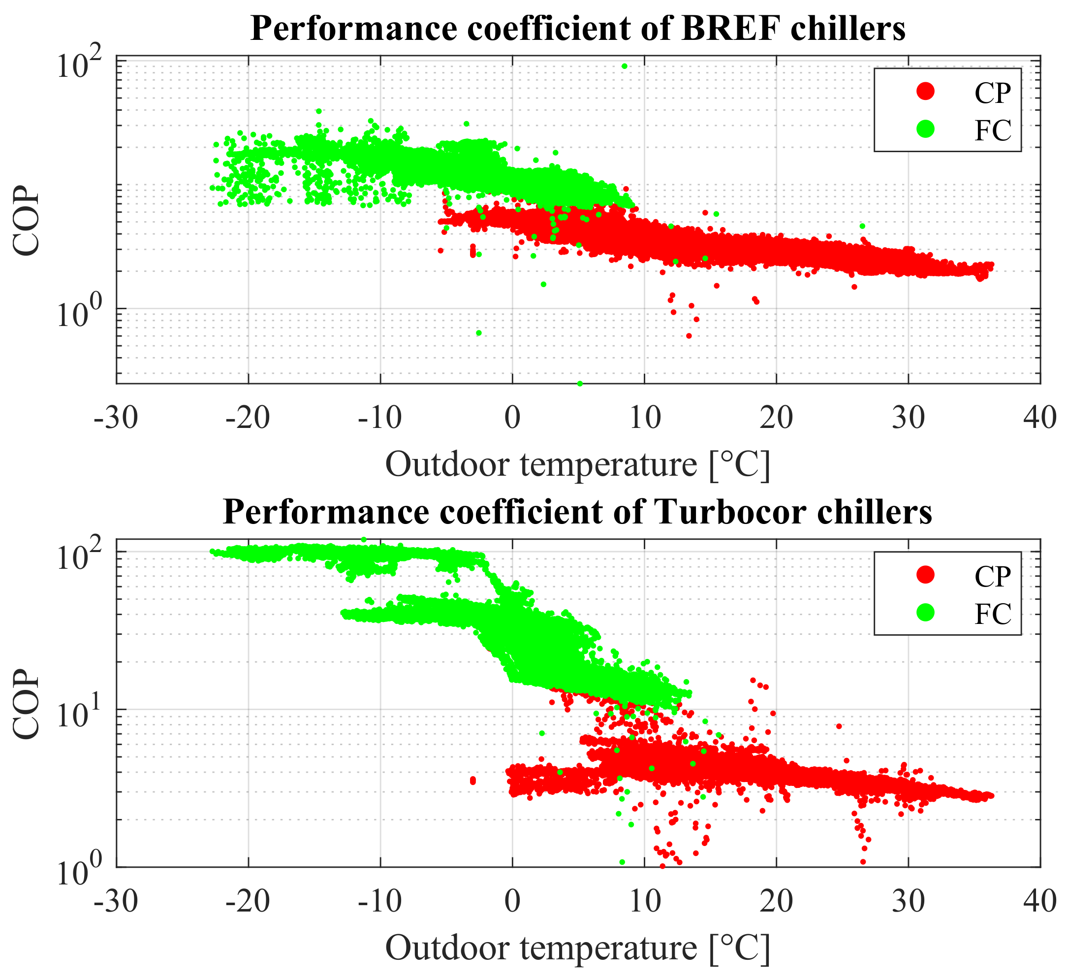
4. Detailed Analysis of a Few Cases under the Proposed Control Strategy

4.1. Change in Cooling Power Demand

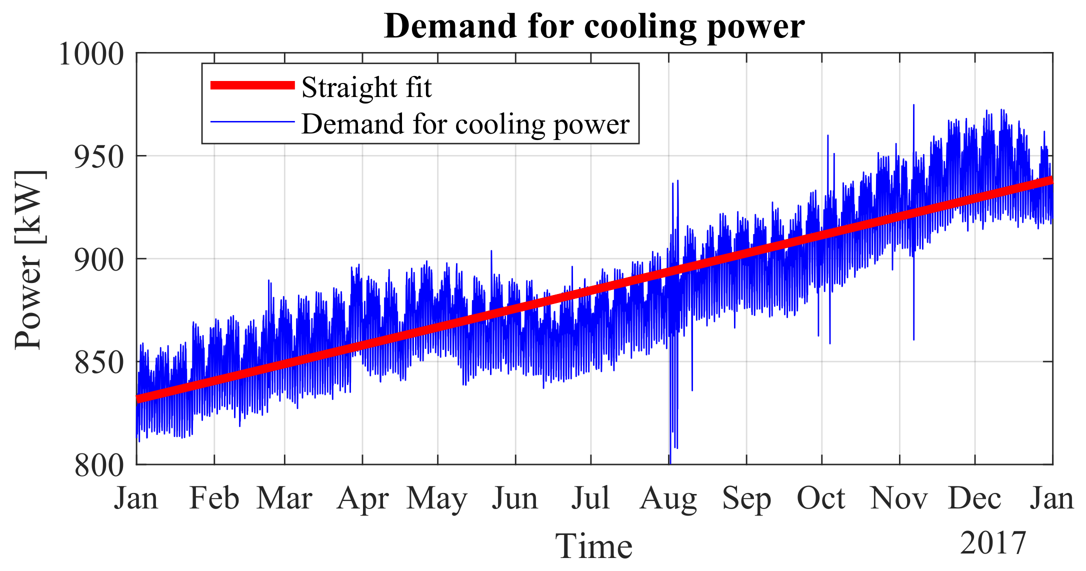
When analyzing the data on the cooling capacity needs of the data center (see Figure 8) in 2017, it was found that, with the exception of May–June, the demand grew over time. At the beginning of the year, it averaged 832 kW, and at the end of the year it increased to an average of 939 kW. This means an increase in 106 kW (13%) over the year. The increase in demand for cooling capacity resulted from the increase in the amount of IT equipment installed in the server room. The average annual cooling capacity requirement was 855 kW. The demand for cooling capacity was approximated by a straight line with a slope coefficient of 0.001 and a shift of 832. The straight fit ratio was 0.89.

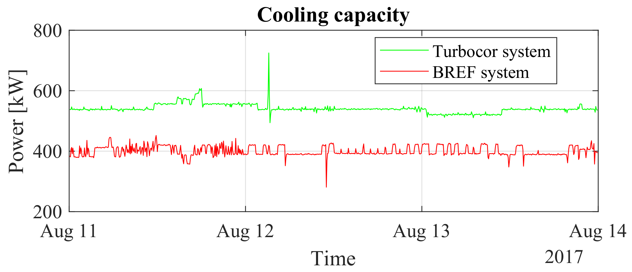
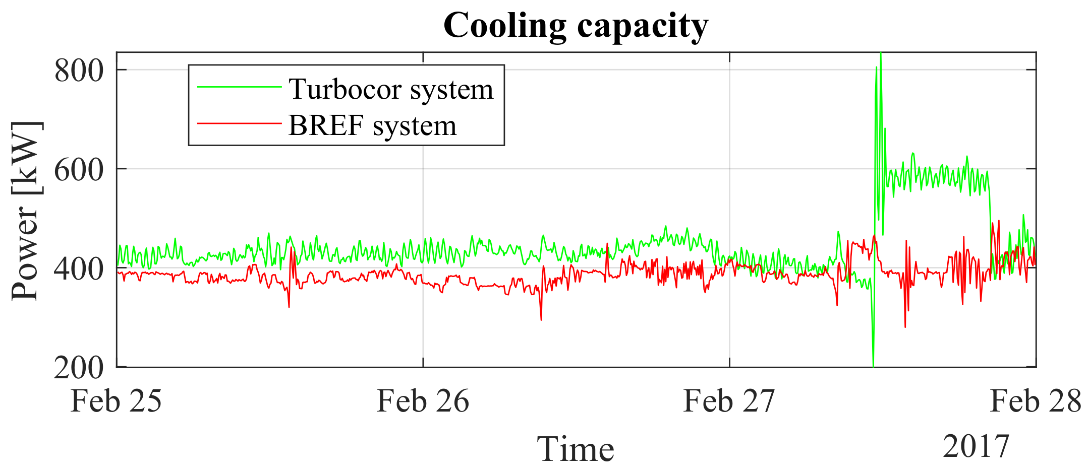
4.2. Comparison of Chillers’ Capacities by Operating Modes

Figure 9 shows the capacity of the entire cooling system and the capacities of the BREF and Turbocor systems. On average, the annual efficiencies of the BREF and Turbocor systems were 396 and 496 kW, respectively.

The operation of the BREF system in FC mode was possible until mid-May and from mid-October. The Turbocor system operated in FC mode every month of the year, except that between June and August the freecooling time was negligible. The cooling capacity of the BREF system in both CP and FC modes did not differ by more than 50 kW. In the second half of the year, the cooling capacity of the Turbocor system, operating in FC mode, was lower by as much as 150 kW than in CP mode.

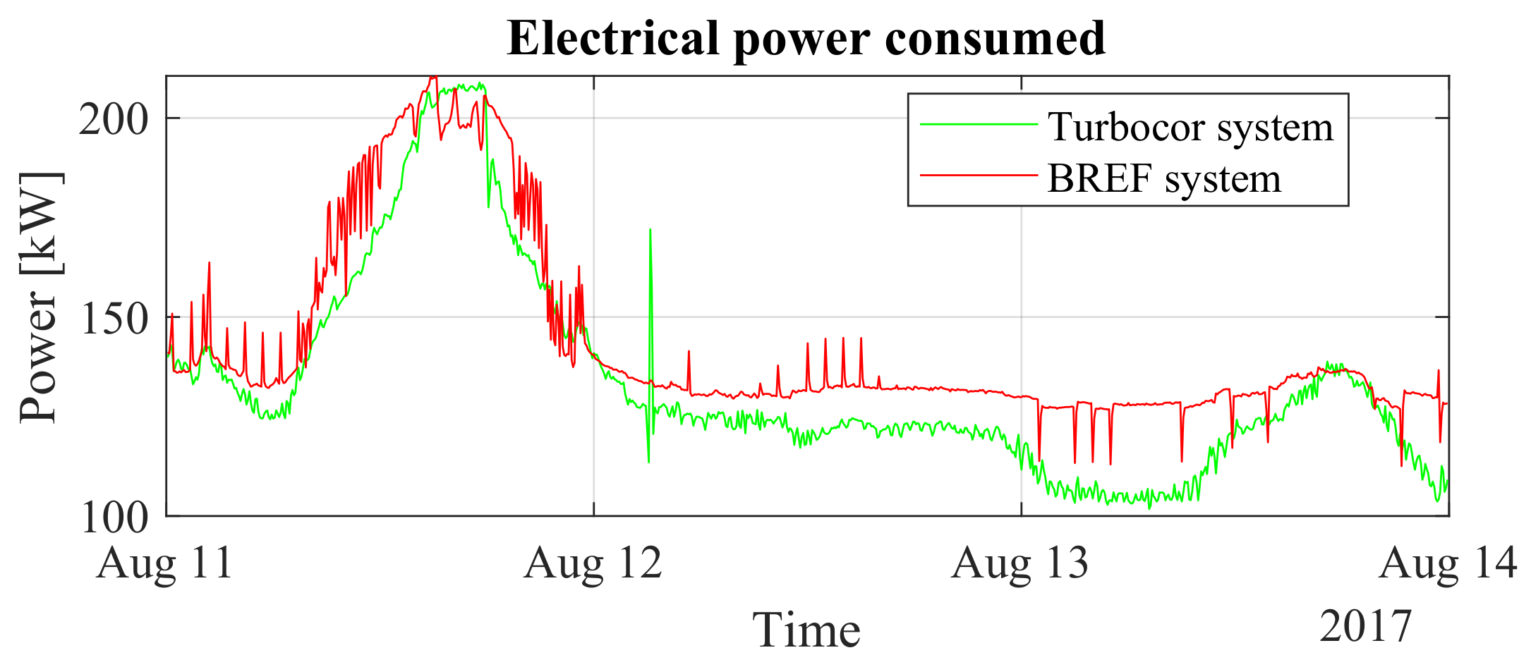
4.3. Comparison of Electric Power Consumption of Chillers by Operating Modes

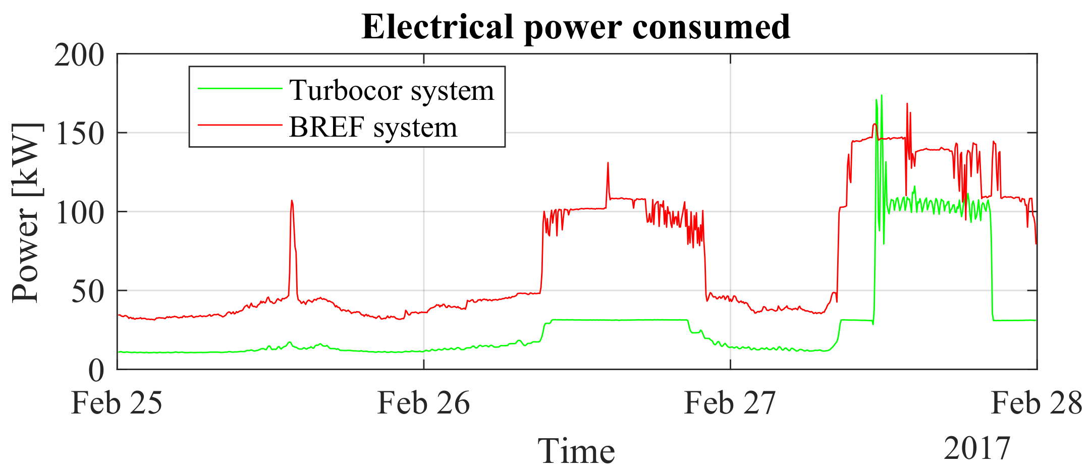
Figure 10 shows the power consumption of BREF units and Turbocor units.

In order to characterise the power consumption profiles of chillers, taking into account the operating mode, the following characteristic values were determined for each operating mode: minimum value, average value, maximum value and amplitude.

Table 3. Power consumption parameters of cooling systems by operating modes.

Operating Mode	Minimum	Mean	Maximum	Amplitude
BREF system
FC	19.70 kW	35.60 kW	58.60 kW	38.90 kW
CP	52.30 kW	116.80 kW	210.60 kW	158.30 kW
FC & CP	19.70 kW	92.37 kW	210.60 kW	190.90 kW
Turbocor system
FC	3.99 kW	21.74 kW	32.90 kW	28.91 kW
CP	73.91 kW	122.73 kW	224.45 kW	150.54 kW
FC & CP	3.99 kW	68.53 kW	224.45 kW	220.46 kW

presents these parameters.

When analyzing the power consumption of both types of chillers operating in CP mode, it was determined that the average power consumption levels of the chillers were similar (116.8 kW for BREF and 122.73 kW for Turbocor). However, taking into account that the cooling capacity of the Turbocor chillers in this mode was higher, their energy efficiency was also 22% higher than that of BREF the chillers (see

Table 4. Momentary COP profile parameters of cooling systems by operating modes.

Operating Mode	Minimum	Maximum	Amplitude
BREF system
FC	7.2	27.1	19.9
CP	1.9	6.2	4.3
FC & CP	1.9	27.1	25.2
Turbocor system
FC	10.7	109.1	98.4
CP	2.6	5.4	2.8
FC & CP	2.6	109.1	106.5

).

The advantage of the Turbocor units, in turn, is more evident in the FC mode. The average power consumption in this mode is 39% lower than the average power consumption of BREF units (35.6 kW for BREF units and 21.74 kW for Turbocor units). Worth noting is the very low power consumption of the Turbocor system operating in FC mode in the first half of January (from 6 January 2017 to 11 January 2017). Due to extremely low outside temperatures, the average power consumption during these days was 4.2 kW (81% less than the average FC consumption of 21.7 kW). At that time, there were no drift fans, because the convection of heat from the drift to the air itself was sufficient, there being no need to force the air flow with the fans. In addition, the capacity of the circulation pump was reduced, which reduced the power consumption. For the BREF system, the reduction in power consumption during this period of time was not so noticeable. The average power consumption for the BREF system over that period of time was 22.9 kW (36% less when compared to the average freecooling consumption of 35.6 kW). The reason was a smaller capacity reserve, which made it impossible to stop the fans, and the design of the unit, which requires the operation of two circulation pumps in FC mode.

There is no difference between the maximum power consumption in FC mode and the minimum power consumption in CP for a BREF system. The power profile is strictly monophonic between compressor and freecooling operation. This is made possible by the design of the unit, which has separate air exchangers dedicated to FC and CP modes, so they can operate simultaneously. In this case, we have a situation where the BREF system, working in CP mode, is also supported by freecooling coolers. We could call this an intermediate (mixed) mode. Due to the lack of sufficient historical data, this mode is not listed separately in the graphs but is classified as compressor mode because a refrigerant compressor was already operating in this mode.

The difference between the maximum power consumption in FC mode and the minimum power consumption in CP mode is very large for the Turbocor system, at 41 kW. The reason is the two-state process of switching between modes of operation. The Turbocor system can only function in two operating modes: compressor or freecooling. There is no mixed mode. The reason for this is a single air exchanger (drycooler). In an instant, it is therefore possible to dissipate heat in CP and FC mode.

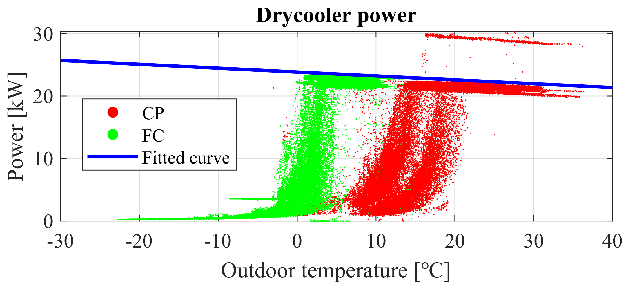
4.4. Power Consumption of the Turbocor System Drycooler

Figure 11 shows the electric power consumption of the drycooler (drycooler fans) as a function of the outside temperature. At outdoor temperatures below −20 ${}^{°}$C, the power consumption of the drycooler reached a minimum of 250 W. This is the idle power consumption of the electronics themselves in the fans and the drift controller. The fans did not rotate at such low outside temperatures.

The power consumption of the drycooler increases with the outdoor temperature up to 23.48 kW at 4.1 ${}^{°}$C. Then, as the outside temperature increases, the maximum power consumption decreases (see the straight limit line). The reason for the maximum power consumption of the drycooler decreasing as the temperature increases is the decrease in air density as its temperature increases, and thus the decrease in the resistance of the fan rotor operation at a given speed. Thanks to a simple approximation, it can be assumed that at the temperature of −30 ${}^{°}$C, the power consumption of a drycooler would be 25.7 kW, and at the temperature of +40 ${}^{°}$C it would be 21.4 kW. The power consumption was approximated by a straight line with a slope coefficient of −0.0622 and a shift of 23.84. The straight fit ratio was 0.78.

Most of the year, the drycooler worked with a limited maximum fan speed of 90% of the nominal speed. Operation with limited maximum revolutions corresponds to all points below the straight line. Due to the high outdoor temperatures at the turn of July/August, the fan operating limit was raised to 100% of the nominal speed. The corresponding points are above the straight line. Limiting the maximum speed of the fans to 90% of the nominal speed allowed us to reduce the instantaneous power consumption by 7.2 kW, compared to fans operating at the nominal speed. This reduced the annual electricity consumption of the drycooler by 10.3 MWh.

5. Analysis of the COP Coefficient

The key to the use of a cooling system is its coefficient of performance. Its improvement was the main objective of modernizing the cooling system. The data presented in Figure 12 show that this objective was achieved. Table 4 presents the statistical parameters of the momentary COP profile.

All coefficients (except for the maximum COP in compressor mode) improved for the Turbocor system compared to the BREF system. The reason why the Turbocor system achieved a lower maximum COP for compressor operation is that the BREF system operated partially in mixed mode (during compressor operation it was additionally supported by freecooling coolers). In addition, it worked in compressor mode at temperatures for which the Turbocor system had already switched to freecooling mode.

The annual average COP for the Turbocor system was 4.30 for the compressor mode, 21.55 for the FC mode and 7.24 for both modes of operation. The annual average COP for the BREF system was 3.42 for the CP mode, 10.83 for the FC mode and 4.28 for both modes of operation. The percentage increase in the average annual energy efficiency index for the Turbocor system for each mode of operation was determined. For FC mode, the increase was 99% (from 10.83 to 21.55), and for CP mode it was 26% (from 3.42 to 4.30). The average annual energy COP coefficient for both modes of operation increased by 69% (from 4.28 to 7.24). The obtained data on the increase in COP coincide with the research carried out so far [25,26].

The Turbocor system reached a COP of 109.1 at extremely low outside temperatures.

COP Coefficient for the Outdoor Temperature

Figure 13 shows the COP coefficient value in relation to the outside temperature. A greater share of FC mode in the operation of Turbocor units is visible, along with much higher COP values in this mode of operation. Unfortunately, the temperature hysteresis of switching between operating modes is also visible all the time. For the BREF system, it is from −6 ${}^{°}$C to 9 ${}^{°}$C, and for the Turbocor system, from 0 ${}^{°}$C to 12 ${}^{°}$C. For the BREF system, this hysteresis did not cause such a big jump in electricity consumption, because the difference in COP between FC and CP modes is relatively small. For the Turbocor system, on the other hand, this hysteresis had a more negative impact on the level of electricity consumption, as the COP for FC mode is much higher than the COP for compressor mode. Hysteresis reduces the freecooling operation time and thus reduces the share of time with high COP.

6. Detailed Analysis of the Control Scenario at Specific Conditions

From the experimental data set, two critical cases were selected—one for maximal outdoor temperatures, and the second for when the switching between cooling modes occurred.

6.1. Case Study of Cooling Systems’ Operation during Maximal Outdoor Temperature

When selecting the time range for analysis, the condition was set that it should be a period in which the momentary outdoor temperature was close to the annual maximum, and at the same time, the amplitude of the temperature course was at least 20 ${}^{°}$C. These conditions were met by the time range analyzed in this section. Thanks to the appropriate range of outdoor temperatures, it is possible to show and compare the specificity of the operation of cooling systems in summer, operating in compressor mode. Graphs are presented showing the outdoor temperature, the electric power consumed, the generated cooling power and the COP coefficient.

6.1.1. Outdoor Temperature

Figure 14 shows the course of outdoor temperature from 11 to 13 August 2017. The 11 August was a high-temperature day; the subsequent days were colder. The maximum temperature during this period was 35.9 ${}^{°}$C, the minimum was 11.7 ${}^{°}$C, the average was 18.8 ${}^{°}$C and the amplitude was 4.2 ${}^{°}$C.

6.1.2. Electrical Power Input

Figure 15 shows the power consumption profiles of the cooling systems in operation from 11 to 13 August 2017. During the whole period, both systems were in compressor mode. The characteristic values of the power curves are presented in

Table 5. Parameters of the power consumption profiles on 11–13 August 2017.

System	Minimum	Mean	Maximum	Amplitude
BREF	112.5 kW	143.2 kW	210.6 kW	98.0 kW
Turbocor	101.8 kW	133.6 kW	208.9 kW	107.1 kW

.

The power consumption levels of the systems on 11 August 2017 were similar. There was a greater oscillation of the power consumption of the BREF system. The reason was the stepping by the step control of the BREF compressor’s capacity in steps 0–25–50–75–100%. The Turbocor system is able to regulate the capacity of the compressors linearly. For this reason, its power consumption profile is less volatile over short periods of time.

On 12 August 2017, the power consumption of the Turbocor system decreased in relation to the power consumed by the BREF system. This was due to a lower outside temperature than on the previous day. This regularity was most evident in the first half of 13 August 2017 (the temperature at that time reached a minimum of 11.7 ${}^{°}$C). The power consumption of the Turbocor system was reduced by 24 kW during this period.

6.1.3. Cooling Capacity

Figure 16 shows the course of the cooling capacity of each cooling system from 11 to 13 August 2017. The cooling capacity of the BREF system can be considered as constant during this period. The reason for the occurring capacity spikes was the unobtrusive value of compressor capacity control. This is due to the design of the BREF compressor units, and it is not possible to adjust the capacity linearly.

The performance of the Turbocor system was set at 540 kW. There were two deviations from this value: the first one at 11.30 on 11 August to 1.50 on 12 August, and the second one from 00.30 on 13 August to 11.00 on 13 August.

The first was the result of the high outside temperature, which made it difficult for the BREF system to keep its cooling capacity at 400 kW, and at the extreme point (16:00) its capacity dropped to 360 kW. The cooling capacity shortfall had to be filled by the Turbocor system, which reached 607 kW at its peak.

The second deviation was due to the low outside temperature and the BREF system, which at low outside temperatures produces excess cooling capacity, THEREBY reducing the load on the Turbocor system.

6.1.4. COP Coefficient

The COP of cooling systems is shown in Figure 17. The COP coefficient of the Turbocor system is higher than the COP of the BREF system FOR the whole interval. This difference is particularly visible for the low outdoor temperatures, to which the Turbocor system reacted positively by significantly increasing its COP, whereas the increase in the COP of the BREF system is less noticeable. Detailed data are presented in

Table 6. COP profile parameters on 11–13 August 2017.

System	Minimum	Mean	Maximum	Amplitude
BREF	1.7	2.9	3.4	1.7
Turbocor	2.7	4.2	5.2	2.5

.

6.2. Comparative Analysis of the Operation of Cooling Systems on 25–27 February 2017

When selecting the time range for analysis, the condition was set that it should be the period in which the momentary outdoor temperature allows for the analysis of the switching moment between the operating modes, and at the same time when the amplitude of the temperature course was at least 20 ${}^{°}$C. These conditions were fulfilled by the time range analyzed in this section. The appropriate range of outdoor temperatures allows one to show and compare the specificity of the operation of cooling systems in spring and autumn, switching between modes of operation. Graphs are presented showing the outdoor temperature, the electric power consumed, the generated cooling power and the COP coefficient.

6.2.1. Outdoor Temperature

Figure 18 shows the course of outdoor temperature on 25–27 February 2017. The day of February 25 was a low-temperature day; the subsequent days were warmer. The maximum temperature during this period was 19.1 ${}^{°}$C, minimum −3.8 °C, average 4.0 ${}^{°}$C and amplitude 22.9 ${}^{°}$C.

6.2.2. Electrical Power Input

Figure 19 shows the power consumption of the cooling systems. Thanks to the appropriately selected time interval, the operation of the systems in both modes of operation: compressor and freecooling can be observed.

The Turbocor system worked exclusively in FC mode from 25 to 26 February. The relationship between an increase in outside temperature and an increase in electrical power consumption is visible. Between 10:00 and 23:00 on 26 February, there was constant power consumption by the Turbocor system at 31 kW. The reason for this situation was the continuous operation of the system at maximum efficiency (drycooler fans operate at maximum speed at all times). The drift controller made the decision to fully control the fans; however, the superior building management control system did not make the decision to switch the system into compressor mode because the outside temperature limit was not exceeded. This temperature limit was exceeded on February 28 at 11:15, which is visible in the graph as a sudden increase in the power consumed to the value of 174 kW. Until 12:15, power consumption above 120 kW was observed. The reason for the high power consumption during this period was the cooling down of the chilled water to the nominal temperature. The chilled water temperature rises above the nominal temperature when switching the Turbocor system between operating modes because the switching interrupts the cooling energy production. After 12:15, power consumption stabilized at an average level of 104 kW until 20:30, where it switched to FC mode. The BREF system operated in compressor mode every day. On 25 February, from 13:20 to 14:10, compressor operation took place; on 26 February, from 9:00 to 22:00, compressor operation took place; and on 27 February, from 11:10 till the end of the day, compressor operation took place. On 26 February, the differences in freecooling operation of the Turbocor and BREF systems were clearly visible. The Turbocor system was operating 24 h a day in FC mode and the BREF system only for 11 h. Detailed parameters of the electrical power consumed are presented in

Table 7. Electric power consumption on 25–27 February 2017.

System	Minimum	Mean	Maximum	Amplitude
BREF	31.3 kW	69.9 kW	168.5 kW	137.2 kW
Turbocor	10.5 kW	29.4 kW	173.8 kW	163.3 kW

.

6.2.3. Cooling Capacity

The cooling capacities of the systems on 25–26 February were similar (see Figure 20). The average cooling capacities during these days were as follows: 431 kW for the Turbocor system and 381 kW for the BREF system. At the beginning of 27 February, the Turbocor system’s performance began to drop until 11:10, when the Turbocor was switched to compressor mode. Compressor operation took place until 20:25, and the average capacity in this mode was 588 kW.

6.2.4. COP Coefficient

The average COP of the Turbocor system was 3.4 times higher than the average COP of the BREF system in the analyzed period. Detailed data are presented in

Table 8. COP profile parameters on 25–27 February 2017.

System	Minimum	Mean	Maximum	Amplitude
BREF	2.4	7.3	12.7	10.4
Turbocor	4.1	24.9	41.6	37.5

. Figure 21 shows the change in the COP value over time. When analyzing the chart, it was found that the low outdoor temperature caused a significant increase in the COP of the Turbocor system. For the BREF system, this increase was less noticeable.

6.2.5. Outdoor Temperature When Switching from Freecooling Mode to Compressor Mode with the Turbocor System

In order to verify the correct operation of the control algorithm, Figure 22 was analyzed, showing the maximum daily outside temperatures prevailing at the time of switching the Turbocor system from FC mode to CP mode.

The points in Figure 22 indicate the outside temperature when the Turbocor system exited FC mode (switching to CP mode). The line indicates average temperatures over a given period of time. The year is divided into three periods in which the average outside temperatures were 12.9, 12.4 and 10.5 ${}^{°}$C, respectively. During the year of 2017, two changes were made to the system switching temperature. At the beginning of the year, the temperature was 13 ${}^{°}$C. On 19 July it was lowered to 12.5 ${}^{°}$C, and on 7 October it was lowered again to 10.5 ${}^{°}$C. The reason for the reductions was a continuous increase in demand for cooling capacity in the server room. The lowering of the switching temperature was done manually on the basis of observation by the facility staff.

The reduction resulted in an increase in power consumption in the temperature range where the cooling system no longer operated in FC mode. From 19 July to 7 October, this temperature range was between 12.4 and 12.9 ${}^{°}$C. Temperatures in this range occurred during this period of time for 49 h. Based on the analysis of historical data, it was assumed that in this temperature range the Turbocor system would consume an average of 32 kW per hour of electric power when operating in FC mode. In fact, while working in compressor mode, it consumed an average of 119 kW of electric power per hour. The difference in average power consumption was 87 kW. For a period of 49 h, this resulted in an increase of 4263 kWh in electricity consumption.

On 7 October, the threshold temperature for switching the system between operating modes was lowered from 12.4 to 10.5 ${}^{°}$C. The outdoor temperature was in this range for 72 h, from 7 October to the end of the year. The Turbocor system, working in this temperature range in FC mode, would consume an average of 31 kW of electrical power. After changing the switching temperature limit, it was already operating in compressor mode, drawing an average of 115 kW of electric power. The difference in average power consumption was 84 kW. For a period of 72 h, this resulted in an increase of 6048 kWh in electricity consumption.

Decreasing the outside temperature at which the system switches between operating modes results in increased electricity consumption. In 2017, the related losses totaled 10.3 MWh. These losses, resulting from an increase in the demand for cooling capacity with a constant maximum capacity of the freecooling cooling system, were the basis for expanding the system to increase its cooling capacity. Usually, such expansion takes place at a time when the costs associated with increased electricity consumption are so high that the return on investment becomes profitable for the company.

6.2.6. Outdoor Temperature When Switching from Freecooling Mode to Compressor Mode with the BREF System

In order to compare the outside temperature limits for freecooling operation of the Turbocor system and the BREF system, the temperatures at which the unit exited FC mode operation and switched to CP mode were also determined for the BREF system. The data are shown in Figure 23.

A much larger scatter of the points in relation to the Turbocor system is visible (see Figure 22). The line, approximating temperature points, has a positive slope coefficient. One could conclude from this that the BREF system was operating in FC mode at higher outside temperatures at the end of the year, despite increased demand for cooling capacity. However, the slope of the straight line is relatively small and its values at the beginning and end of the year differ by only 1 ${}^{°}$C (4.58 ${}^{°}$C—beginning of the year, 5.41 ${}^{°}$C—end of the year). The standard deviation of the data is 14.1. Taking all these observations into account, it was concluded that the variability of the data was so high that it was not possible to determine the trend of temperature changes in the exit from the BREF FC mode. The only reliable evaluation indicator was the average exit temperature of 5.0 ${}^{°}$C.

6.3. Analysis of the Energy Efficiency of the Entire Cooling System

The above work presented data on cooling sources (chillers). A detailed analysis of the entire system was not carried out (thus the electricity consumed by the precision air conditioning cabinets was not included in the work). However, to be able to compare the new cooling system with other systems described in the literature, the current subsection presents data on the electric power consumption and the COP coefficient of each system, taking into account the electric power consumed by precision air-conditioning cabinets (see

Table 9. Electric power consumption and COP parameters of the cooling systems by operating mode in year 2017.

Operating Mode	Mean Power	Mean COP
BREF system
FC	68.60 kW	5.39
CP	149.80 kW	2.67
FC & CP	125.37 kW	3.15
Turbocor system
FC	54.74 kW	8.56
CP	155.73 kW	3.39
FC & CP	101.53 kW	4.89

).

The estimated value of the COP index in terms of the entire system determined as an annual average was 4.89. Referring to the comparative comparison of various cooling system solutions presented in the works [11,27], it can be noted that the estimated value of the COP index is higher than those of the systems tested by Mongia et al. (3.7) and Trutassanawin et al. (3.2); lower than that of Marcinichen et al. (7.0); and within the range described by Choi et al. (3.2–9.0). Modernization of the control system and cooling sources increased the COP of the entire system by 55%.

7. Conclusions

Limitations in the comprehensive solutions for cooling systems commonly available on the market allowed the development of a unique and dedicated solution taking into account the specific climatic conditions of our data center’s configuration. Analysis of the work of a productively working server room allowed for the individual selection of cooling system components and the design of a dedicated control system. The assumed modernization goal, which was to extend the system’s operating time in freecooling mode, was achieved. The designed solution was subjected to long-term annual production tests to obtain data illustrating the operation of the cooling system in various operating conditions.

The developed solution allowed us to reduce the electricity consumption of the cooling system by 206.9 MWh or 67% during 2017, which translated into a reduction in electricity costs by €9869 (based on EUROSTAT; the average price of 1 MWh of electricity was assumed to be €47.7). The electricity consumption needed to produce 1 MWh of cooling energy was reduced from 0.17 MWh to 0.05 MWh (see

Table 10. System’s power and energy statistic for outdoor temperatures corresponding to Turbocor freecooling operation.

BREF System	Turbocor System
Mean of electrical power and energy
66 kW	22 kW
310.3 MWh	103.4 MWh
Annual savings in energy	206.9 MWh (67%)
Mean of cooling power and energy
386 kW	456 kW
1815 MWh	2144 MWh
Specific electrical energy required to produce 1 MWh of cooling energy
0.17 MWh	0.05 MWh
Improve	0.12 MWh (71%)

). Significant increases in the annual average coefficient of performance of 99% in FC mode, 26% in CP mode and 69% in both modes were achieved, and the annual operating time in FC mode increased by 23.6% (see Figure 24).

The rule-based nature and transparency in the sequence of state changes of the control system enabled its precise diagnostics and reliable operation throughout the year. Further research on the control system will aim to develop a controller incorporating a greater number of inputs and state variables in order to obtain a variable switching point between operating modes maximizing the operating time of the cooling plant in freecooling mode.