A Deep Learning Method Based on Bidirectional WaveNet for Voltage Sag State Estimation via Limited Monitors in Power System

Abstract

Voltage sag state estimation on the basis of a limited number of installed monitors is essential to dividing the responsibility for the voltage sag and taking corresponding measurements for improvement in voltage quality. Therefore, a deep learning methodology via bidirectional WaveNet for the voltage sag state estimation is proposed in this paper. The presented method can simultaneously estimate voltage sag state at non-monitored buses via limited monitors. Especially, the proposed deep learning method using the bidirectional WaveNet is designed to explore the long-term and long-range temporal dependencies in both the forward and backward directions. In this way, only by using original measured voltages through monitors, high accuracy for voltage sag state estimation can be achieved without restructured or redesign of the raw monitored data. An excellent advantage of the presented algorithm is that it can be implemented without system parameters or operating conditions or any other prior information. The presented methodology was verified by the IEEE 30-bus benchmark system. The experimental results illustrated that the accuracy of the voltage sag state estimation results was over 99.83%. Furthermore, a comparison among different models, including the bidirectional GRU-based model, one-way WaveNet-based model, and bidirectional WaveNet-based model, was also conducted. The results illustrated that the proposed bidirectional WaveNet-based model achieved the highest accuracy and quickest convergence speed.

1. Introduction

Due to the fact of increasing access to sensitive loads of the power grid, voltage sag is attracting more attention from both industry and academia [1]. Actually, voltage sag is considered one of the most serious power quality problems [2]. Both voltage sag state estimation (VSSE) and voltage sag level assessment (VSLA) are essential for designing a mitigation plan, evaluating the economic cost, verifying the responsible parties, and taking corresponding measurements for improving voltage quality. Especially, the VSLA can be regarded as a statistical measure of VSSE, where VSSE is usually denoted by voltage amplitude or voltage range, and VSLA is normally represented by the System Average Interruption Frequency Index (SARFI). In other words, VSLA can be easily predicted as long as a VSSE result is achieved. Therefore, research on VSSE calculation is of great importance.

In general, the VSSE problem can be mainly divided into the following two categories: model-based estimation and data-based estimation.

In the model-based estimation method, fault type and fault position should be determined first through circuit analysis, followed by VSSE [3,4,5,6,7]. For example, in [3], the VSSE is achieved via Bayesian inference, where some prior information, including fault position and other power system parameters or operating conditions, is necessary. It is observed that the model-based VSSE method can obtain voltage sag magnitude [4]. However, for such approaches, network parameters or operating conditions, such as system topology, line impedance, fault type, fault location, and fault impedance, are strongly required [5,6]. Moreover, as mentioned in [7], the estimation performance is severely dependent on the selection and number of fault positions.

In fact, huge numbers of monitors or measurement equipment have already been distributed in modern power system and, therefore, massive data have been accumulated [8]. Unfortunately, above presented model-based estimation method cannot fully take advantage of the abundant information implied among historical measurement records or data. Hence, recent research has shown a trend of solving the VSSE problem by using measured voltages, which denotes the data-based method for VSSE solution [9,10,11].

Theoretically, for a power system, monitors or measurements could be placed at all nodes, under which case every voltage sag state at each node can be estimated directly. However, it is not feasible for economic causes. It is common that only limited monitors could be installed at specific nodes. Therefore, it would be of great use to realize VSSE at non-monitored buses with these accessible monitored voltages via limited number [12]. This is just the purpose of our work to be solved in this paper, which can obtain the VSSE of the whole power system only by using measured data via limited monitors.

Different from the above model-based method, in the data-based estimation method, the VSSE problem can be processed only by using the available measured voltages from monitors or data acquisition system without requiring any information on network parameters or operating conditions. The data-based method can effectively avoid the difficulty in locating fault positions. Given fault probabilities, for most approaches in recent literatures, probabilistic analysis has been implemented. For instance, in [9], a probabilistic analysis based on the correlation among the System Average RMS Frequency Index (such as SARFI-90 or SARFI-70) was proposed, where the System Average RMS Frequency Index at different buses were estimated. Apparently, probabilistic analysis was more suitable for VSLA, rather than VSSE. The main reason lies in the fact that the dynamics between voltage sag states at different times cannot be fully captured in this way. Actually, the VSSE results constantly varied from time to time. Hence, temporal characteristics should be involved for accurate VSSE, which is also difficult for a model-based method since the underlying physics is unknown. This is just where deep learning finds its role for the VSSE solution. Deep learning can fully learn the sequential feature from measured data without requiring any simplifications or assumptions of the system’s physical model. In [10], a VSSE approach based on deep learning is proposed to estimate voltage ranges for six sag categories regardless of fault location or characteristics. However, it has been verified that the selection of input features into deep neural networks, as well as the construction or format of the input data, greatly impacts estimation results. In addition, for each deep learning model in [10], the VSSE result at only one specific bus, rather than multiple interesting buses, can be analyzed simultaneously.

A deep learning method based on bidirectional WaveNet (Bi-WaveNet) is proposed for a VSSE solution in this paper. The corresponding contributions are listed as follows:

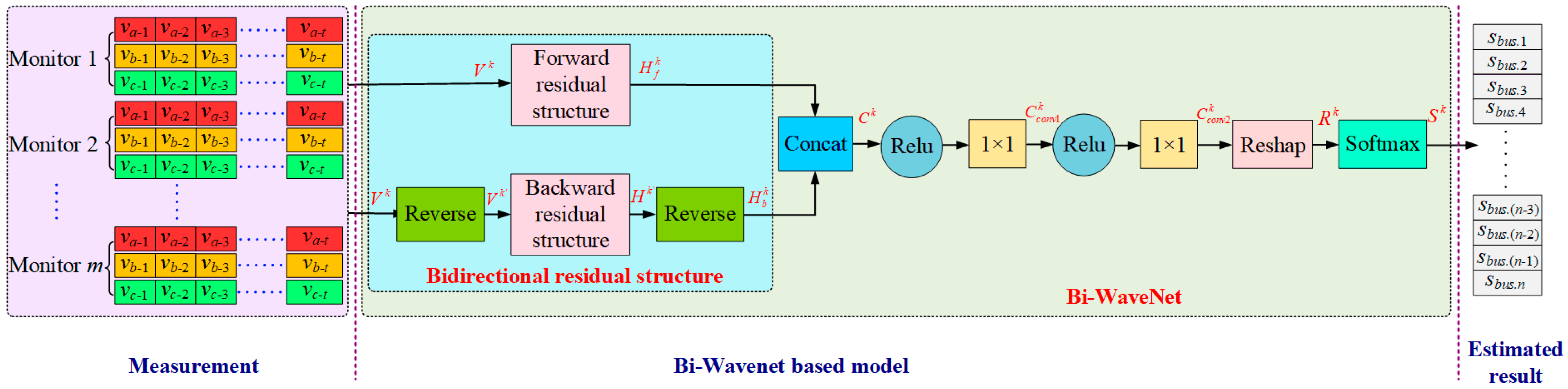
• A deep learning architecture via Bi-WaveNet was designed to explore the long-term and long-range temporal dependencies in both the forward and backward directions;
• Original measured voltages through limited monitors, without restructuring of the raw monitored data, can be directly used for feature extractions with high accuracy;
• Only with a single model, the VSSE results at multiple non-monitored buses can be simultaneously estimated;
• The effectiveness of the Bi-WaveNet-based algorithm was further compared with other methods including the one-way WaveNet-based method and the Bi-GRU-based method. The results illustrated that the Bi-WaveNet-based model could achieve the highest accuracy and quickest convergence speed.

The remaining sections of this paper are conducted as follows. In Section 2, the VSSE problem is described; then, the reason for choosing WaveNet is introduced, followed by the proposed architecture. In Section 3, the corresponding experimentation is conducted to examine the model’s performance. Finally, the discussion and conclusion are drawn in Section 4 and Section 5, respectively.

2. Proposed Method

In this section, the definition of the VSSE problem discussed in this paper is firstly described. Then, the reason of choosing WaveNet is given, followed by a brief introduction to WaveNet and Bi-WaveNet. Finally, the presented deep learning methodology via Bi-WaveNet is demonstrated.

2.1. Problem Description

Voltage sag is defined as power-quality issues with voltage amplitude being 0.9~0.1 p.u. of the nominal value for a period of 0.5~30 cycles. In power system, monitors cannot be installed at all buses for economic causes, and only limited meters are assembled at specific buses. Therefore, as illustrated in Figure 1, only by using measured voltages from limited monitors, the VSSE result at non-monitored buses can be simultaneously estimated.

In detail, the VSSE problem discussed here is defined to classify the voltage magnitudes at non-monitored buses into several classes with specific voltage magnitude ranges. Moreover, in the IEEE Std 1668^TM-2017, a histogram of data collected from the DPQII study illustrates that voltage sag magnitude is less likely to fall in the range of (0 p.u., –0.5 p.u.) [13]. Hence, the VSSE result is classified into the same category if the voltage magnitude range of (0 p.u., 0.5 p.u.). Meanwhile, referring to [10], the VSSE result was uniformly divided into 5 intervals if the voltage magnitude was greater than or equal to 0.5 p.u. Therefore, the VSSE result was generally classified into 6 categories.

In Figure 2, a color scale was also adopted to clearly mark different categories. As demonstrated in Figure 2, it can be observed that the VSSE result was classified into Category 1 (colored by red), if the voltage magnitude at the non-monitored bus was greater than or equal to 0.9 p.u. Similarly, the VSSE result was classified into Category 2 (colored by yellow-green), if the voltage magnitude range at the non-monitored bus was [0.8 p.u., 0.9 p.u.). The VSSE result is classified into Category 3 (colored by green), if the voltage magnitude range at the non-monitored bus is [0.7 p.u., 0.8 p.u.). The VSSE result is classified into Category 4 (colored by blue), if the voltage magnitude range at the non-monitored bus is [0.6 p.u., 0.7 p.u.). The VSSE result is classified into Category 5 (colored by purple), if the voltage magnitude range at the non-monitored bus is [0.5 p.u., 0.6 p.u.). And, the VSSE result is classified into Category 6 (colored by rose-red), if the voltage magnitude range at the non-monitored bus is (0 p.u., 0.5 p.u.).

In essence, the VSSE problem is aimed at establishing the nonlinear relationship between given the input and the expected output, where the given input is the measured voltage from limited meters and the expected output is the VSSE results of the non-monitored buses. Furthermore, an important characteristic of this problem is that the VSSE result can be solved directly from voltage measurement without requiring any prerequisites such as system parameters, and operating condition.

2.2. Reason for Choosing WaveNet

As previously mentioned, some model-based estimation methods have been proposed to solve the VSSE problem. However, much prior network information (such as fault impedance, fault type, and fault position) is required, whereas these detailed network parameters cannot be obtained easily or directly in most cases.

In fact, the measured voltages via monitors naturally own time series characteristics, while the standard RNN (recurrent neural network) can analyze time series data [14]. Theoretically, the RNN also can be used to solve the VSSE problem, whereas, in practice, long-range temporal dependencies are required for the VSSE solution. In fact, if a standard RNN is employed to handle long sequences, it may face vanishing/exploding gradients difficulty, leading to very slow training [15,16]. To solve this problem, some variants of standard RNNs, including the LSTM (long short-term memory) and the GRU (gated recurrent unit) are presented. In detail, the LSTM cell owns three gates (including the input gate, forget gate, and output gate), and the GRU cell contains two gates (including the update gate and reset gate) [17,18]. Hence, compared with the standard RNN, the LSTM cell and GRU cell commonly achieve better performances: the training converge rate will be faster and temporal dependencies will be considered longer [19]. Note that the LSTM or GRU can alleviate rather than avoid vanishing/exploding gradients problem. Hence, it is still impossible for them to handle even moderately long-term or long-range temporal dependencies. The main reason lies in the fact that for standard RNN or LSTM and GRU, every recurrent neuron receives both the input vector and the output from a previous time step.

Different from the RNN or the LSTM and GRU, the WaveNet has been proposed to avoid vanishing/exploding gradients problem. It is composed of dilated causal convolutional layers enlarging the receptive field by skipping input with a certain step [20]. In fact, the WaveNet has already been confirmed that it is powerful for modeling very long-term temporal dependencies on time series tasks [21]. Therefore, in this paper, the WaveNet was chosen to solve the VSSE problem.

2.3. WaveNet and Bi-WaveNet

The WaveNet network models the joint probability of sequential data as a product of conditional probabilities as follows [22]:

$$p(x)=\underset{t=1}{\overset{T}{\mathsf{\Pi }}}p(x_t|x_1,x_2,\dots \dots ,x_{t-1})$$

(1)

where x, denoted by x = {x₁, x₂, ……, x_t}, is a sequence of data, and T is the total number of input sampling.

The main ingredient of WaveNet are causal convolutions in Figure 3. Obviously, since WaveNet models do not have recurrent connections, it can efficiently avoid the vanishing/exploding gradient problem and typically train faster than the standard RNN and LSTM or GRU, especially when applied to very long sequences. However, for the WaveNet model with convolutional layers, many layers or large filters are required to increase the receptive field. Hence, the dilated causal convolutional layers were further applied by skipping input values with a certain step.

In Figure 4, a stack of dilated causal convolutional layers with the dilation being {1, 2, 4, 8} and the filter length being 2 are demonstrated. Moreover, the residual block is illustrated in Figure 5 based on dilated causal convolutional layers. The one-way WaveNet architecture is illustrated in Figure 6. Especially, in the one-way WaveNet, the residual block and skip connections were employed throughout the network to speed up convergence and enable training of much deeper models.

Although the one-way WaveNet in Figure 6 can process long-term dependencies with high training efficiency, it only has access to learn sequential data through forward direction instead of forward and backward passes, leading to low accuracy for the VSSE results.

In order to solve this problem, a Bi-WaveNet is presented. The Bi-WaveNet is a bi-directional form of one-way WaveNet that learns the input sequence in both the forward and backward directions via forward network and backward network, respectively. Note that the backward residual structure is the same as the forward residual structure. To be specific, if the input sequence data are denoted as {v₁, v₂, ……, v_t}, where t is the length of a sequence in one batch, the forward WaveNet network flows in the forward direction and calculates the forward hidden state {h_f1, h_f2, ……, h_ft}. Meanwhile, the input {v₁, v₂, ……, v_t} is reversed to {v_t, ……, v₂, v₁}, and then the backward WaveNet network flows in the backward direction and calculates the backward hidden state {h_b1, h_b2, ……, h_bt}. Then, the final output of the Bi-WaveNet, as presented in Equation (2), is achieved according to the hidden states {h_f1, h_f2, ……, h_ft} and {h_b1, h_b2, ……, h_bt}.

$$\left[\begin{array}{c}{h}_{f1},h_{f2},\dots \dots ,h_{ft}\\ h_{b1},h_{b2},\dots \dots ,h_{bt}\end{array}\right]$$

(2)

In this paper, the Bi-WaveNet was adopted to explore long-term information in both backward and forward directions from the monitored voltage. As we illustrate later, this helps extract deep futures to improve the final accuracy of the VSSE results.

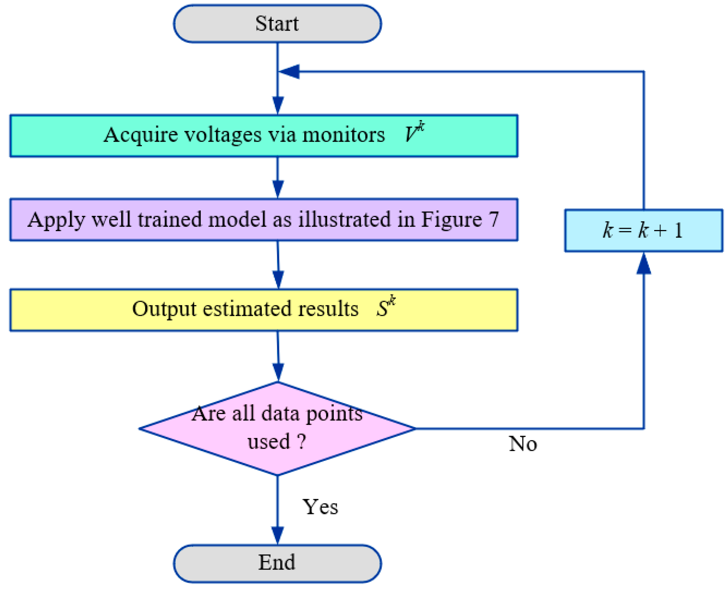
2.4. Proposed Bi-WaveNet Model for VSSE Solutions

As demonstrated in Figure 7, the deep learning architecture of a Bi-WaveNet-based model was proposed for VSSE solutions. In the following illustration, a detail example is demonstrated for specific process.

In general, the input for the Bi-WaveNet-based model is the measured data via monitor 1, 2, ……, m at the monitored buses, and the output is the VSSE results for the non-monitored buses. If the total number of the non-monitored buses to be estimated is n, it is common that m < n. Here, the three-phase voltage magnitude at each monitored node are required. At time k, the Bi-WaveNet-based model input is V^k, as presented in the following Equation (3). The corresponding output is S^k, as illustrated in Equation (5). The proposed Bi-WaveNet is responsible for establishing the nonlinear and deep relationship between the input V^k and the output S^k.

$$\begin{array}{ll}{V}^k& ={[V_1^k,V_2^k,\dots \dots ,V_m^k]}^T\\ & ={\left[\begin{array}{c}{V}_{a1}^k\\ V_{b1}^k\\ V_{c1}^k\end{array}|\begin{array}{c}{V}_{a2}^k\\ V_{b2}^k\\ V_{c2}^k\end{array}|\begin{array}{c}\dots \dots \\ \dots \dots \\ \dots \dots \end{array}|\begin{array}{c}{V}_{am}^k\\ V_{bm}^k\\ V_{cm}^k\end{array}\right]}^T\end{array}$$

(3)

where at time k, $V_1^k$, $V_2^k$, ……, $V_m^k$ denote the measured voltage via monitor 1, 2, ……, m at the metered buses; $V_{a1}^k$, $V_{b1}^k$, and $V_{c1}^k$ are the voltage amplitudes of phases a, b, and c collected by monitor 1, respectively; $V_{a2}^k$, $V_{b2}^k$, and $V_{c2}^k$ are the voltage amplitudes of phases a, b, and c collected by monitor 2, respectively; and, similarly, $V_{am}^k$, $V_{bm}^k$, and $V_{cm}^k$ are the voltage amplitudes of phases a, b, and c collected by monitor m, respectively.

Furthermore, each element in Equation (3) can be written as:

$$\begin{array}{l}{V}_{am}^k={[v_{am\_1}^k,v_{am\_2}^k,\dots \dots ,v_{am\_T}^k]}^T\\ V_{bm}^k={[v_{bm\_1}^k,v_{bm\_2}^k,\dots \dots ,v_{bm\_T}^k]}^T\\ V_{cm}^k={[v_{cm\_1}^k,v_{cm\_2}^k,\dots \dots ,v_{cm\_T}^k]}^T\end{array}$$

(4)

where T is called time steps, and it can be defined as the product of the number of sampling points in one cycle and the number of periods; for monitor m, the $V_{am\_1}^k$, $V_{am\_2}^k$, ……, $V_{am\_T}^k$ denote the measured voltage magnitude of phase a at time steps 1, 2, ……, T; and similarly, the $V_{bm\_1}^k$, $V_{bm\_2}^k$, ……, and $V_{bm\_T}^k$ denote the measured voltage magnitude of phase b at time steps 1, 2, ……, and T; $V_{cm\_1}^k$, $V_{cm\_2}^k$, ……, and $V_{cm\_T}^k$ denote the measured voltage magnitude of phase c at time steps 1, 2, ……, and T.

$$S^k={[S_{bus.1}^k,S_{bus.2}^k,\dots \dots ,S_{bus.n}^k]}^T$$

(5)

where S^k is the calculated VSSE results of the non-monitored buses 1~n at time k via the Bi-WaveNet model (illustrated in Figure 7); in detail, at time k, the $S_{bus.1}^k$, $S_{bus.2}^k$, ……, and $S_{bus.n}^k$ are the VSSE results of the non-monitored buses 1~n, respectively.

To be specific, the shape of V^k is defined as [Batch_size, T, m × 3], where the Batch_size denotes the number of periods for the measured voltage in one batch, and T refers to the sampling points in one cycle. According to Figure 7, the V^k is directly fed into the bidirectional residual structure, where the V^k shall be reversed to $V^{k{}^{\prime }}$, according to the following Equations (6) and (7).

$$V^{k{}^{\prime }}={[V_m^k,\dots \dots ,V_2^k,V_1^k]}^T$$

(6)

$$\begin{array}{l}{V}_{am}^{k{}^{\prime }}={[v_{am\_t}^k,\dots \dots ,v_{am\_2}^k,v_{am\_1}^k]}^T\\ V_{bm}^{k{}^{\prime }}={[v_{bm\_t}^k,\dots \dots ,v_{bm\_2}^k,v_{bm\_1}^k]}^T\\ V_{cm}^{k{}^{\prime }}={[v_{cm\_t}^k,\dots \dots ,v_{cm\_2}^k,v_{cm\_1}^k]}^T\end{array}$$

(7)

In detail, the V^k is sent to the forward residual structure, and then the forward hidden state $H_f^k=\left\{h_{f1},h_{f2},\dots \dots ,h_{ft}\right\}$ is obtained via the L layers’ forward residual structure. Meanwhile, the $V^{k{}^{\prime }}$ is introduced to the backward residual structure, and then the backward hidden state $H^{k{}^{\prime }}=\left\{h_{bt},\dots \dots ,h_{b2},h_{b1}\right\}$ is obtained via the L layers’ backward residual structure. After, the $H^{k{}^{\prime }}$ is further reversed to $H_b^k=\left\{h_{b1},h_{b2},\dots \dots ,h_{bt}\right\}$. Finally, the concat transform is adopted to combine the $H_f^k$ and the $H_b^k$ according to Equation (2), which is also regarded as the output of the bidirectional residual structure C^k. Here, the shape of C^k is designed as [Batch_size, T, n_dilated × 2], where n_dilated denotes the number of dilated convoluted layer’s neurons of forward residual structure or backward residual structure.

$$C^k=\left[\begin{array}{c}{h}_{f1},h_{f2},\dots \dots ,h_{ft}\\ h_{b1},h_{b2},\dots \dots ,h_{bt}\end{array}\right]$$

(8)

After, the output C^k is further sent to the ReLU activation unit and the 1 × 1 convolution layer, which has a size of 1 × 1 and a depth of 2 (bidirectional residual structure). Here, the shape of $C_{conv1}^k$ (namely, the output of the 1 × 1 convolution layer in Figure 7), is [Batch_size, T, n_{1D conv}], where n_{1D conv} represents the number of neurons of the 1 × 1 convolution layer.

Next, the output, $C_{conv1}^k$, is further sent to another ReLU activation unit and the 1 × 1 convolution layer for nonlinear transformer. Here, the shape of $C_{conv2}^k$ is [Batch_size, T, n_buses × n_categories], where n_nodes is the number of the non-monitored buses to be estimated in the whole power system, and the n_categories is the categories number indicating the VSSE results. According to Figure 2, it is obvious that n_categories is equal to 6.

Then, the Reshape layer is adopted to shape $C_{conv2}^k$ to R^k, which has a shape that is [Batch_size, T, n_buses, n_categories], as expected by SoftMax. Finally, the n_categories (namely, the last dimension of R^k in Figure 7) is introduced to the SoftMax layer, where the Argmax operation is employed to determine the VSSE results according to measurements via limited monitors in the power system.

As a result, the VSSE results of the non-monitored buses can be directly estimated only by using the measured voltage of the monitored buses. The whole flow chart for the VSSE in practical field is demonstrated in Figure 8. The step-by-step procedure is illustrated as follows.

Step 1: For monitored buses, the original three-phase voltages are acquired and sampled to form a series of time sequence data, which is denoted as [$V_1^k$, $V_2^k$, ……, $V_m^k$] in Equation (3). In our studies, all data were from simulations, whereas, in reality, the data can be acquired from power quality monitors, voltage sensors, or other measurement units.

Step 2: The data [$V_1^k$, $V_2^k$, ……, $V_m^k$] are then divided into three parts: training data, validation data, and testing data. The training data are employed to train presented deep learning model as presented in Figure 7, where parameters or hyper-parameters are optimized using the back-propagation through time strategy [23]. Note that this training stage is an offline process. After, the validation data are applied to assess the whole performance of the trained model. If the performance is satisfied, go on to next step for online estimation with the new data. Otherwise, redefine the model and repeat the process until a satisfactory performance is achieved.

Step 3: Since the model has already be trained well with the optimized parameters or hyper-parameters in Step 2, it can be applied directly in the practical field for estimating voltage sag states [$S_{bus.1}^k$, $S_{bus.2}^k$, ……, $S_{bus.n}^k$) of non-monitored buses 1~n as described in Equation (5). To be specific, the data [$V_1^k$, $V_2^k$, ……, $V_m^k$] are immediately sent to the well-trained deep learning model as presented in Figure 7. Here, the [$V_1^k$, $V_2^k$, ……, $V_m^k$] is batched and normalized, and then, the deep and the multi-aspect characteristics are extracted automatically without requiring any prerequisites. It is necessary to mention that the original measured voltages, without restructuring or redesigning, can be directly used for VSSE estimation with high accuracy. The main reason lies in the fact that the presented Bi-WaveNet-based model can explore the long-term and long-range temporal dependencies in both the forward and backward directions.

3. Experimentation and Results

In the following section, the performance of the proposed methodology through the standard IEEE 30-bus system is presented, and meanwhile, the performance is analyzed and compared with other methods or models.

3.1. Data Set Description

As shown in Figure 9, the IEEE 30-bus system with six sources and 30 buses was adopted to confirm the performance of our proposed model. Here, it should be mentioned that both the number and placement of monitors are definitely important for satisfactory VSSE results. Actually, the best VSSE results will be achieved if monitors are installed at all buses. However, it is not economical and unfeasible in the practical field. It may be reasonable to install only a limited number of meters to meet the requirement that the whole power system is observable. Referring to [24], we chose 4 m for observability of the whole power network, which were distributed at bus 2, bus 15, bus 21, and bus 25 (as highlighted by red in Figure 9).

In the following studied cases, all data were generated through MATLAB software simulation, where fault impedance, fault type, and fault location could be considered [14]. For each simulation, fault resistance, ground resistance, sag duration, active power, and reactive power were randomly changed within a certain range. In detail, the range of the fault resistance was within [0.1 Ω, 10 Ω], the range of ground resistance was within [0.01 Ω, 5 Ω], the range of sag duration was within [10 ms, 0.6 s], and the range for active power and reactive power was within [0.95 p.u., 1.05 p.u.], respectively. Numerous simulations were operated to generate the data set.

All data were then complementarily separated into three parts: training set, validation data, and testing set. Here, 70% of the simulated data were adopted for model training. After training, 20% of the simulated data were employed to access performance. Finally, if the performance was satisfied, 10% of the simulated data were employed for testing. Otherwise, the model should be redefined and the process repeated.

Since voltage sag is mostly caused by faults, the following faults, including single-line grounded faults (SLGFs), line-to-line faults (LLFs), line-to-line grounded faults (LLFs), three-phase faults (3PFs), were separately simulated at each line considering different fault resistances, transition resistance, etc. Specifically, each sample in the data set consisted of a given input and a corresponding output, where the input meant the input for the proposed model, and it was represented by measured three-phase voltage at monitored buses via monitors; meanwhile, the output denoted the output for the proposed model, and it was represented by the voltage magnitude range at non-monitored buses. The input can be regarded as a 12-dimensional vector (that is, 3 × 4 = 12), since 4 m were installed in the IEEE 30-bus system. The output can be regarded as a 22-dimensional vector, if the VSSE at the other 22 non-monitored buses (that is bus 3, bus 4, bus 6, bus 7, bus 9, bus 10, bus 12, bus 14, bus 16, bus 17, bus 18, bus 19, bus 20, bus 22, bus 23, bus 24, bus 25, bus 26, bus 27, bus 28, bus 29, and bus 30) were determined.

3.2. Verification for Effectiveness of the Proposed Model

In this paper, the method was examined using the TensorFlow software with Anaconda Python 3.6.8 [23]. All tests were conducted on a workstation that was equipped with a GTX 1080 Ti × 2 graphics processing unit and an Intel i7-8700K processor.

It has already been confirmed that cross-validation is beneficial to alleviate or even avoid model overfitting problems. In other words, cross-validation is useful for examining generalization performance for new data [25]. Hence, in the following test, a five-fold cross-validation methodology was adopted to verify the effectiveness of the presented deep learning model in Figure 7. To be specific, all of the generated data set in Section 3.1. was firstly separated into complementary subsets. Then, the above subsets were combined in different ways, where some parts were used to train the model, and the remaining parts were employed to validate the model.

Furthermore, in order to evaluate the VSSE’s performance from the perspective of quantitative analysis, Accuracy and Loss are defined in Equations (9) and (10).

$$Accuracy(\%)=\frac{N_{correct}}{N_{total}}\times 100$$

(9)

where N_correct is the number of correct VSSE results, and N_total is the number of total tests.

$$Loss=-{\displaystyle \sum _{i=1}^M{\displaystyle \sum _{l=1}^L{s}_l^i\log ({\widehat{s}}_l^i)}}$$

(10)

where M and L are the number of samples and VSSE categories, respectively. The $s_l^i$ is equal to 1 if the sample i is classified in correct class l; otherwise, it is equal to 0. The ${\widehat{s}}_l^i$ is the output of SoftMax in Figure 7, and it can be regarded as the probability of sample i being classified in category l. Obviously, the Loss will become 0, and the Accuracy will reach 100% if the VSSE estimated results becomes close to real values.

The relationship between epochs and loss for VSSE is indicated in Figure 10. From Figure 10, it can be seen that the Bi-WaveNet-based model (marked by the blue line) converged gradually with a steady decreasing loss. In detail, for the Bi-WaveNet-based model, the loss value achieved 5 × 10⁻⁶ with only 10 epochs required. Then, the loss value approached to 10⁻⁸, which can be regarded as the best system performance. These results demonstrate that not only the Bi-WaveNet-based model could be trained robustly, but it could also achieve a relatively low loss.

Further, Figure 11 shows the relationship between epoch and accuracy for the VSSE. As illustrated in Figure 11, it can be observed that the accuracy was higher than 99.83% for the Bi-WaveNet-based model (marked by the blue line). However, in [10], if phase voltages v_a, v_b, and v_c were used directly as model inputs, the accuracy for the method in [10] could only reach 17.7%. This is because, in Reference [10], the phase voltages must be restructured before being fed into the CNN network so as to take advantage of the structure recognition capacity in CNNs. Whereas, for our proposed Bi-WaveNet-based network, good performance can be achieved even if the measured data, v_a, v_b, and v_c, are adopted directly without restricting or design, reducing complexity.

Moreover, further comparisons with other methods were also analyzed to examine the performance of our presented methodology. In [9], a Bayesian filtering method was proposed to solve the VSSE of non-monitored buses, whose accuracy was 97.7%, where fault impedance, fault location, and other prerequisites were required. In order to reduce the requirement of prior conditions for VSSE estimation, in [26], a voltage sag estimation method by requiring system impedance was proposed. Whereas, for our proposed Bi-WaveNet-based model, only by using the original measured voltages through limited monitors, without any prerequisite or other information, the VSSE can be directly estimated with accuracy achieving 99.83%.

In order to further confirm the performance of the presented Bi-WaveNet model, it was compared to the bidirectional gated recurrent unit (Bi-GRU)-based model and the one-way WaveNet-based model, respectively. As clearly demonstrated in Figure 10 and Figure 11, the following conclusions can be further drawn:

(1)

From Figure 10, the loss with the proposed Bi-WaveNet model was less than that of the model based on Bi-GRU and one-way WaveNet. Specifically, the minimum loss value of the Bi-WaveNet model could achieve 1 × 10⁻⁸, whereas, the minimum loss value of Bi-GRU model and one-way WaveNet could only achieve 5 × 10⁻⁴ and 1 × 10⁻⁵, respectively. This means that the deep relationship or function between the monitored voltage and VSSE results can be more accurately extracted by the Bi-WaveNet model, consequently obtaining higher accuracy for VSSE. The main reason for this result is that the Bi-WaveNet can process both forward and backward information;

(2)

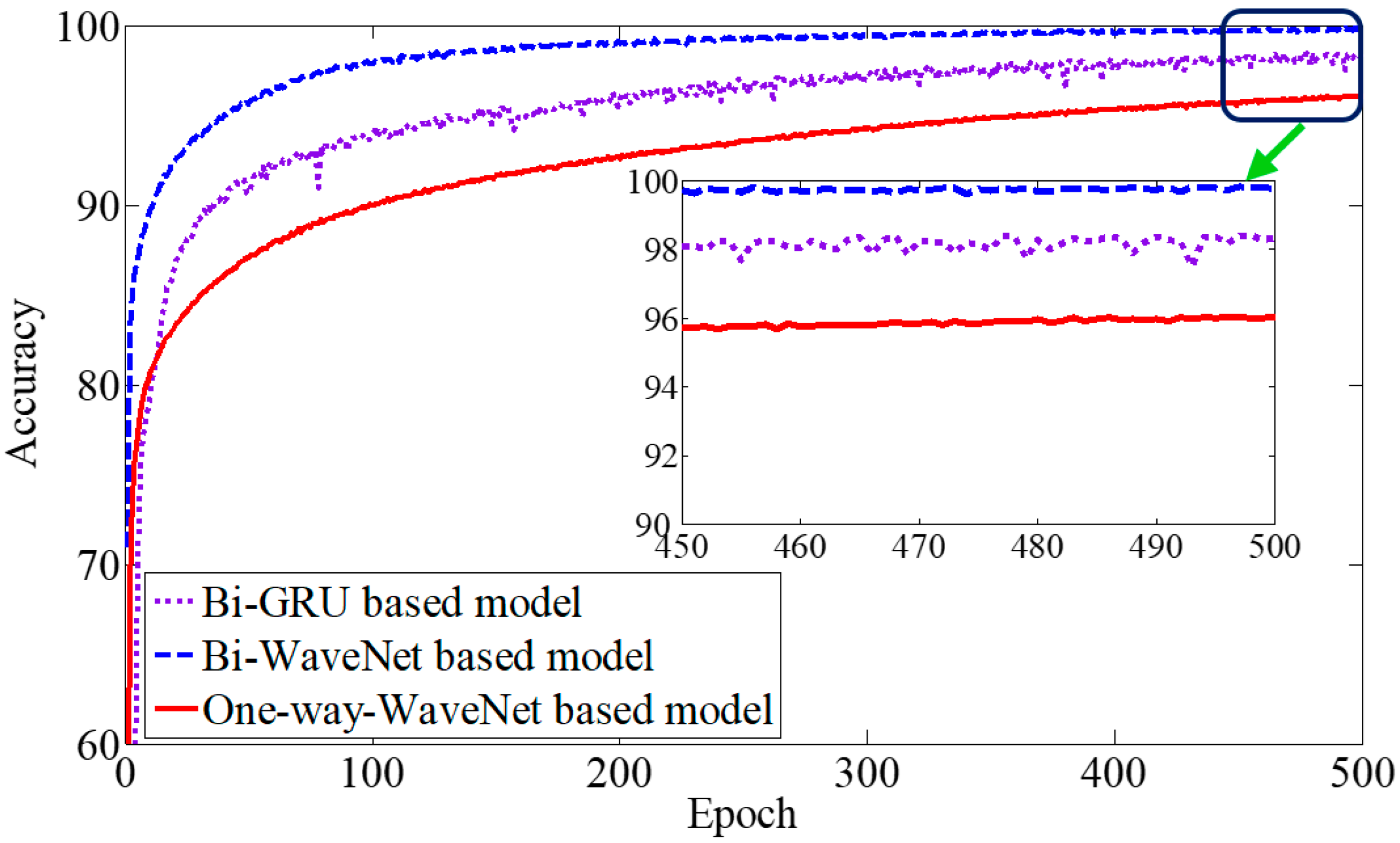
The accuracy of the one-way WaveNet-based model (marked by the red line) was nearly 96%, approximately 4% lower than the Bi-WaveNet-based network (marked by the blue line). This is because the Bi-WaveNet-based network can learn input sequential data in both the forward and backward directions, leading to high accuracy.

(3)

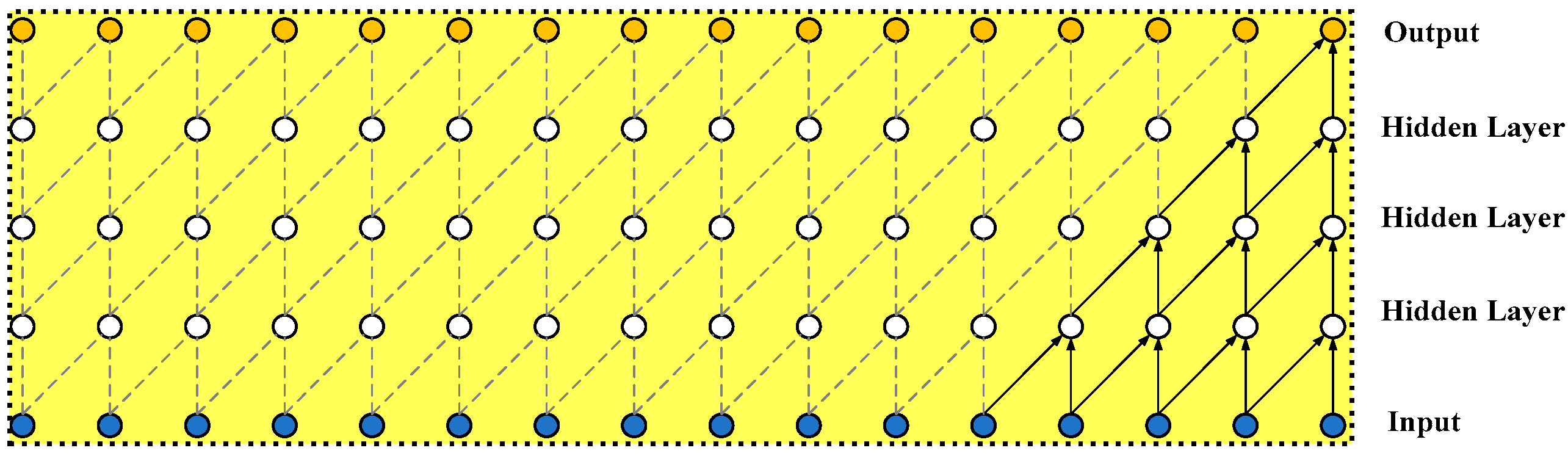
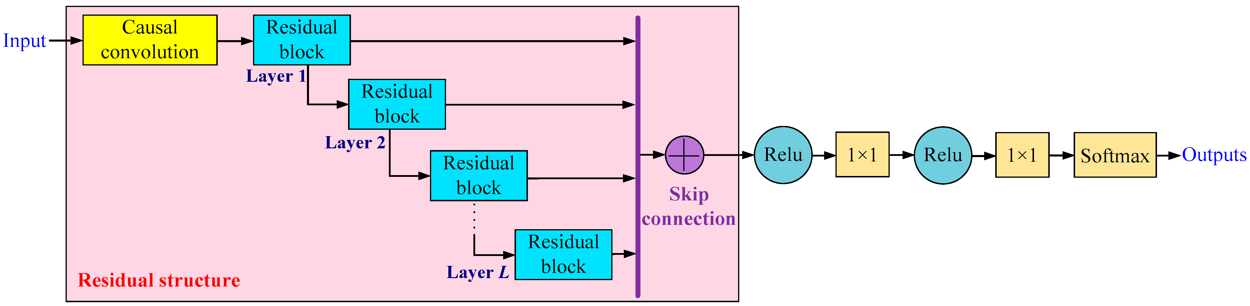
The accuracy of the Bi-GRU-based model was nearly 98% (marked by the purple line), approximately 2% lower than the Bi-WaveNet-based network (marked by the blue line). This was due to the fact that the WaveNet network, based on causal convolutions (as illustrated in Figure 3) and dilated causal convolutions (as demonstrated in Figure 4), can exhibit very large receptive fields to deal with long-range temporal dependencies, resulting in high accuracy.

(4)

Compared with the Bi-GRU (marked by the purple line) and one-way WaveNet (marked by the red line), the convergence speed of the Bi-WaveNet-based model accelerated dramatically. This was because the proposed Bi-WaveNet consists of stacked dilated causal convolution layers, and each causal convolutional layer can process its input in parallel, making the proposed Bi-WaveNet avoid vanishing/exploding gradient problems efficiently, leading to the fastest convergence rate.

Furthermore, Figure 12 demonstrates a graphical illustration of the presented approach if a three-phase grounded short circuit occurs at line 16 in an IEEE 30-bus system. Here, in Figure 12a, the “▲” denotes the measured residual voltage via meters at bus 2, bus 15, bus 21, and bus 25 through simulation. Meanwhile, by using MATLAB/Simulink, the “●” is the simulated voltage magnitude at other non-monitored buses (that is bus 3, bus 4, bus 6, bus 7, bus 9, bus 10, bus 12, bus 14, bus 16, bus 17, bus 18, bus 19, bus 20, bus 22, bus 23, bus 24, bus 25, bus 26, bus 27, bus 28, bus 29, and bus 30). Furthermore, all these simulated voltage magnitudes at non-monitored buses (denoted by “●”) can be divided into six categories according to Figure 2, which can be considered as theoretical values. Moreover, in Figure 12b, the point (denoted by “*”) is the theoretical category according to Figure 12a, and the bar is the estimated category via our proposed model in Figure 7. From Figure 12, it is obvious that the VSSE results at the non-monitored buses can be accurately estimated via limited monitors in power system.

In order to further evaluate the performance of the proposed model in Figure 7, another set of 2400 new samples, which has never been used before, was employed. The confusion matrix is demonstrated in Figure 13, with an overall accuracy of 99.92%. Moreover, as clearly shown in Figure 13, we can further analyze the distribution of faulted estimation of the VSSE results. It was obvious that four out of the six categories can be estimated with 100% accuracy; meanwhile, the VSSE accuracies of the other two categories were both 99.75%. In detail, the first row of Figure 13 suggests that for the true category T₁, there should be, in total, 399 + 1 = 400 voltage sags located within the voltage magnitude range being greater than or equal to 0.9 p.u. However, 399 out of 400 were correctly recognized, and the other one was in the fault estimated range [0.8 p.u., 0.9 p.u.). The fifth column in Figure 13 indicates that for the estimated category E₅, the voltage magnitude range was [0.5 p.u., 0.6 p.u.), the estimated voltage magnitude ranges were accurately recognized with 99.75% certainty: ($\frac{400}{400+1}\times 100\%=99.75\%$). Here, in 0.25% ($\frac{1}{400}\times 100\%=0.25\%$) of the tests, the true VSSE result should be (0 p.u., 0.5 p.u.), which deviated from the estimated range [0.5 p.u., 0.6 p.u.).

3.3. A Comparison among Different Monitor Placement

The fundamental condition for satisfactory VSSE performance of proposed model in Figure 7, is that the measured voltages input [$V_1^k$, $V_2^k$, ……, $V_m^k$] via monitors 1~m, as described in Equation (3), can detect all sag in the estimated power system. In other words, only a limited number of monitors are distributed at some specific buses to satisify the requirement of observability. In our work, the methodology in [24] is chosen as reference for monitor placement. Moreover, the impacts of different monitor placement on accuracy of VSSE results are verified, as demonstrated in

Table 1. The accuracy for different monitor placement.

Monitor Placement	Number of Monitors	Accuracy of VSSE Result (%)
18, 24, 25	3	63.21
15, 22, 25	3	75.90
15, 22, 27	3	86.33
2, 15, 21, 25	4	99.83
2, 15, 18, 21, 25	5	99.87
2, 15, 16, 21, 25	5	99.91
2, 5, 15, 16, 21, 25	6	99.95

.

As apparently illustrated in Table 1, the following conclusions can be drawn:

(1)

In general, along with increasing the number of monitors, the accuracy of the VSSE results improved sharply. The main reason lies in the fact that more monitors means redundant data and sufficient information;

(2)

However, once the number of monitors attains a certain value, the accuracy of the VSSE results improves slowly, even if the number further increases. Therefore, there should be a balance between installation costs, computational burden, accuracy, and complexity. Here, we chose the number of monitors to be four;

(3)

Both the number of monitors and the detailed allocation of them are equally important. For the allocation of 18, 24, and 25 and the allocation of 15, 22, and 25, different allocations with the same number of monitors produced different accuracies in the VSSE results. Whereas, for the placement 2, 15, 16, 21, and 25 and the placement 2, 15, 18, 21, and 25, it was observed that different allocations with the same number of monitors achieved similar accuracies in the VSSE results. This is because the detailed placement of monitors should be distributed to ensure the observability of the whole power network;

(4)

For monitor placement 18, 24, and 25, the accuracy of the VSSE results was unsatisfactory. The reason lies in the fact that this monitor placement could not ensure the whole system’s observability, resulting in missing data and insufficient information.

4. Discussion

The VSSE problem was solved from the perspective of data-driven methods, where a deep learning architecture based on the Bi-WaveNet was adopted. In this way, only by directly using original measured voltages through monitors, high accuracy for a VSSE solution can be achieved without restructuring or designing the raw monitored data. The accuracy and robustness were examined in the IEEE 30-bus system. However, there are still some aspects regarding the applicability needed to be further discussed:

(1)

Since abundant high-quality data may be a little difficult to be collected, deep learning methodology depending on small amounts of data will be studied in our future work;

(2)

The monitor placement is important for satisfactory VSSE results. In the further studies, efficient monitor placement, including the number of monitors and their best allocations, will be considered.

5. Conclusions

In this paper, a data-driven approach to estimating voltage sag state in sparsely monitored power systems was presented. In the approach, a deep learning architecture using a bidirectional WaveNet model was proposed, where long-term and long-range temporal dependencies in both the forward and backward directions were explored. Furthermore, the effectiveness and viability of the proposed model were confirmed. The following conclusions can be drawn:

(1)

Only by using measured original voltages via limited monitors, the proposed deep learning architecture via bidirectional WaveNet can simultaneously estimate voltage sag states at multiple non-monitored buses without any prior conditions;

(2)

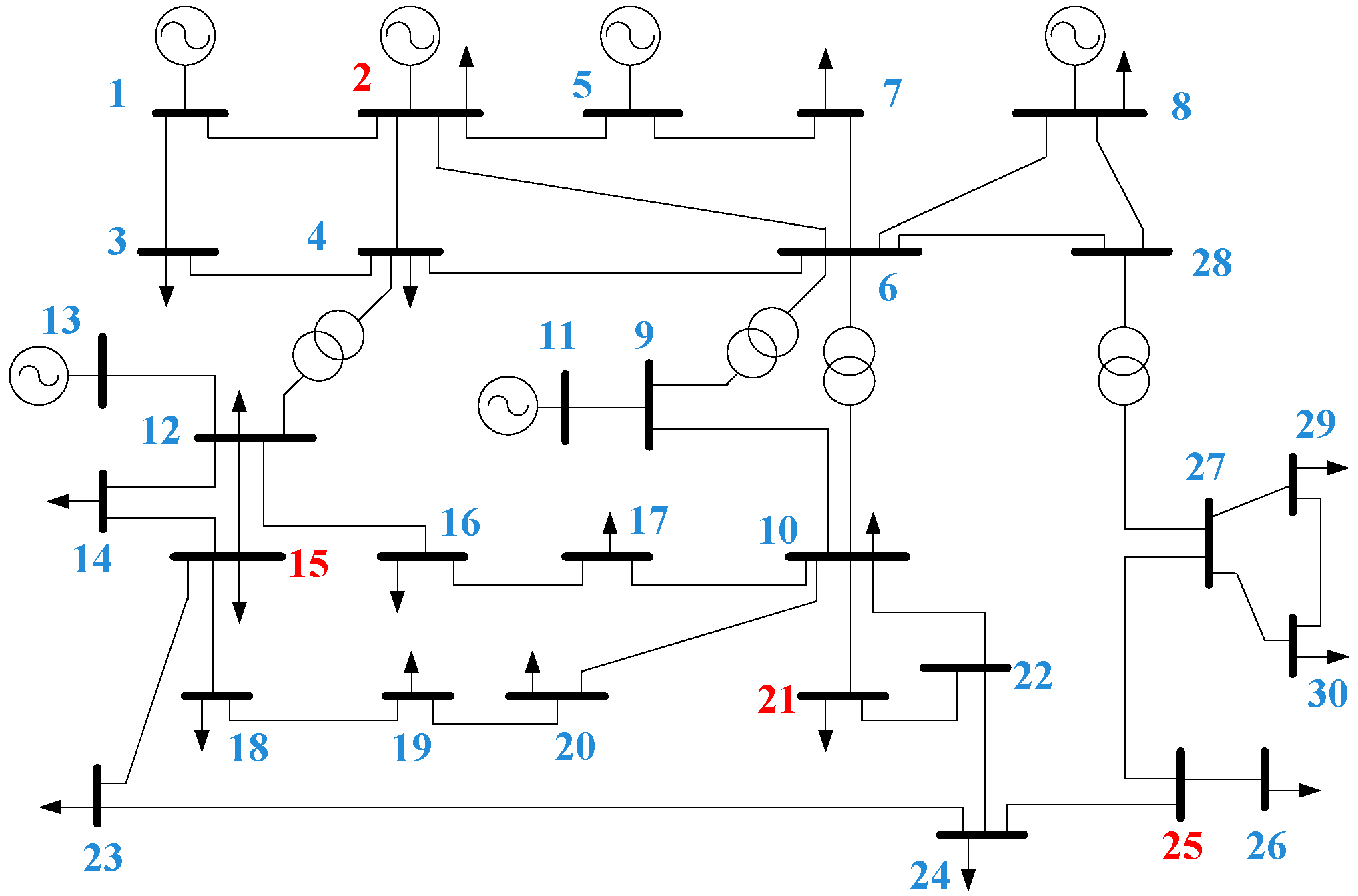
The experiments on IEEE 30-bus system confirmed that the performance of the presented model was satisfactory. The accuracy of the VSSE result was over 99.83%;

(3)

A comparison among different models, including a bidirectional GRU-based model, a one-way-WaveNet-based model, and a bidirectional WaveNet-based model, was also conducted. The results indicate that the proposed bidirectional WaveNet-based model achieved the highest accuracy and quickest convergence speed.

(4)

A comparison among different monitor placements was demonstrated. It illustrated that the optimal number of monitors and their best placement to ensure observability of the power network is a basic requirement to achieve satisfactory accuracy.

References

1. Hasan, S.; Muttaqi, K.M.; Sutanto, D.; Bouzerdoum, A. Calculation of the Voltage Sag Recovery Point-on-Wave and Sag Duration Using System Parameters. IEEE Trans. Ind. Appl. 2020, 56, 4588–4601. [Google Scholar] [CrossRef]
2. Torres, A.P.; Roncero-Sanchez, P.; Batlle, V.F. A Two Degrees of Freedom Resonant Control Scheme for Voltage-Sag Compensation in Dynamic Voltage Restorers. IEEE Trans. Power Electron. 2018, 33, 4852–4867. [Google Scholar] [CrossRef]
3. Ye, G.; Xiang, Y.; Nijhuis, M.; Cuk, V.; Cobben, J.F.G. Bayesian-Inference-Based Voltage Dip State Estimation. IEEE Trans. Instrum. Meas. 2017, 66, 2977–2987. [Google Scholar] [CrossRef]
4. Di, F.; Lijun, T.; Yu, C. Voltage sag state estimation based on Hybrid Particle Swarm Optimization algorithm. In Proceedings of the 2015 IEEE 10th Conference on Industrial Electronics and Applications (ICIEA), Auckland, New Zealand, 15–17 June 2015. [Google Scholar]
5. Blanco-Solano, J.; Petit-Suárez, J.F.; Ordóñez-Plata, G.; Kagan, N.; Almeida, C. Voltage Sag State Estimation using Compressive Sensing in Power Systems. In Proceedings of the 2019 IEEE Milan PowerTech, Milan, Italy, 23–27 June 2019; pp. 508–512. [Google Scholar]
6. Wang, Y.; Li, S.-Y.; Xiao, X. Estimation Method of Voltage Sag Frequency Considering Transformer Energization. IEEE Trans. Power Deliv. 2020, 36, 3404–3413. [Google Scholar] [CrossRef]
7. Di Mambro, E.; Caramia, P.; Varilone, P.; Verde, P. Voltage sag estimation of real transmission systems for faults along the lines. In Proceedings of the 2018 18th International Conference on Harmonics and Quality of Power (ICHQP), Ljubljana, Slovenia, 13–16 May 2018. [Google Scholar]
8. Cruz, I.B.N.C.; Lavega, A.P.; Orillaza, J.R.C. Overview of methods for voltage sag performance estimation. In Proceedings of the 2016 17th International Conference on Harmonics and Quality of Power (ICHQP), Belo Horizonte, Brazil, 16–19 October 2016; pp. 508–512. [Google Scholar]
9. Zambrano, X.; Hernández, A.; Izzeddine, M.; de Castro, R.M. Estimation of voltage sags from a limited set of monitors in power systems. IEEE Trans. Power Deliv. 2017, 32, 656–665. [Google Scholar] [CrossRef]
10. Liao, H.; Milanović, J.V.; Rodrigues, M.; Shenfield, A. Voltage sag estimation in sparsely monitored power systems based on deep learning and system area mapping. IEEE Trans. Power Deliv. 2018, 33, 3162–3172. [Google Scholar] [CrossRef]
11. Espinosa-Juarez, E.; Espinoza-Tinoco, J.R.; Hernandez, A. Neural networks applied to solve the voltage sag state estimation problem: An approach based on the fault positions concept. In Proceedings of the 2009 Electronics, Robotics and Automotive Mechanics Conference (CERMA), Cuernavaca, Mexico, 22–25 September 2009; pp. 88–93. [Google Scholar]
12. Lv, G.; Chu, C.; Zang, Y.; Chen, G. Voltage sag source location estimation based on optimized configuration of monitoring points. CPSS Trans. Power Electron. Appl. 2021, 6, 242–250. [Google Scholar] [CrossRef]
13. IEEE Std 1668–2017 (Revision of IEEE Std 1668–2014); IEEE Recommended Practice for Voltage Sag and Short Interruption Ride-Through Testing for End-Use Electrical Equipment Rated Less than 1000 V. IEEE: Manhattan, NY, USA, 2017. [CrossRef]
14. Deng, Y.; Liu, X.; Jia, R.; Huang, Q.; Xiao, G.; Wang, P. Sag source location and type recognition via attention-based independently recurrent neural network. J. Mod. Power Syst. Clean Energy 2021, 9, 1018–1031. [Google Scholar] [CrossRef]
15. Ma, J.; Liu, H.; Peng, C.; Qiu, T. Unauthorized broadcasting identification: A deep LSTM recurrent learning approach. IEEE Trans. Instrum. Meas. 2020, 69, 5981–5983. [Google Scholar] [CrossRef]
16. Zhao, R.; Wang, D.; Yan, R.; Shen, F.; Wang, J. Machine Health Monitoring using Local Feature-based Gated Recurrent Unit Networks. IEEE Trans. Ind. Electron. 2018, 65, 1539–1548. [Google Scholar] [CrossRef]
17. Yuan, X.; Li, L.; Shardt, Y.A.W.; Wang, Y.; Yang, C. Deep learning with spatiotemporal attention-based LSTM for industrial soft sensor model development. IEEE Trans. Ind. Electron. 2021, 68, 4404–4414. [Google Scholar] [CrossRef]
18. Li, J.; Yang, C.; Yuxuan, L.; Xie, S. A context-aware enhanced GRU network with feature-temporal attention for prediction of silicon content in hot metal. IEEE Trans. Ind. Inform. 2021. [Google Scholar] [CrossRef]
19. Hu, C.; Ou, T.; Zhu, Y.; Zhu, L. GRU-Type LARC Strategy for Precision Motion Control with Accurate Tracking Error Prediction. IEEE Trans. Ind. Electron. 2021, 68, 812–820. [Google Scholar] [CrossRef]
20. Ariav, I.; Cohen, I. An end-to-end multimodal voice activity detection using WaveNet encoder and residual networks. IEEE J. Sel. Top. Signal Process. 2019, 13, 265–274. [Google Scholar] [CrossRef]
21. Juvela, L.; Bollepalli, B.; Tsiaras, V.; Alku, P. GlotNet—A raw waveform model for the glottal excitation in statistical parametric speech synthesis. IEEE/ACM Trans. Audio Speech Lang. Process. 2019, 27, 1019–1030. [Google Scholar] [CrossRef]
22. Sisman, B.; Zhang, M.; Li, H. Group sparse representation with waveNet vocoder adaptation for spectrum and prosody conversion. IEEE/ACM Trans. Audio Speech Lang. Process. 2019, 27, 1085–1097. [Google Scholar] [CrossRef]
23. Deng, Y.; Wang, L.; Jia, H.; Tong, X.; Li, F. A sequence-to-sequence deep learning architecture based on bidirectional GRU for type recognition and time location of combined power quality disturbance. IEEE Trans. Ind. Inform. 2019, 15, 4481–4493. [Google Scholar] [CrossRef]
24. Jiang, H.; Xu, Y.; Liu, Z.; Ma, N.; Lu, W. A BPSO-based method for optimal voltage sag monitor placement considering uncertainties of transition resistance. IEEE Access 2020, 8, 80382–80394. [Google Scholar] [CrossRef]
25. Géron, A. Hands-on Machine Learning with Scikit-Learn and TensorFlow; O’Reilly Media, Inc.: Newton, MA, USA, 2017. [Google Scholar]
26. Hernández, A.; Milanović, J.V. Efficient Monitor Placement and Voltage Sag Estimation Using System Impedance Matrix. In Proceedings of the 2019 IEEE Milan PowerTech, Milano, Italy, 23–27 June 2019; pp. 1–6. [Google Scholar] [CrossRef]
Figure 1. The illustration of the VSSE problem.
Energies 15 02273 g001
Figure 2. The definition of the VSSE result.
Energies 15 02273 g002
Figure 3. Causal convolutional layers.
Energies 15 02273 g003
Figure 4. The dilated causal convolutional layers.
Energies 15 02273 g004
Figure 5. The residual block diagram.
Energies 15 02273 g005
Figure 6. The whole structure of the one-way WaveNet.
Energies 15 02273 g006
Figure 7. The architecture of the Bi-WaveNet-based model.
Energies 15 02273 g007
Figure 8. The flow chart for VSSE in the practical field.
Energies 15 02273 g008
Figure 9. The IEEE 30-bus system.
Energies 15 02273 g009
Figure 10. The relationship between epoch and loss.
Energies 15 02273 g010
Figure 11. The relationship between epoch and accuracy.
Energies 15 02273 g011
Figure 12. The demonstrated result of proposed model: (a) the measured voltage magnitude via meters and simulated voltage magnitude at other non-monitored buses; (b) the theoretical category and estimated category of non-monitored buses.
Energies 15 02273 g012
Figure 13. The confusion matrix on the test set.
Energies 15 02273 g013