Optimal Allocation of Distributed Generators in Active Distribution Networks Using a New Oppositional Hybrid Sine Cosine Muted Differential Evolution Algorithm

Abstract

The research proposes a new oppositional sine cosine muted differential evolution algorithm (O-SCMDEA) for the optimal allocation of distributed generators (OADG) in active power distribution networks. The suggested approach employs a hybridization of the classic differential evolution algorithm and the sine cosine algorithm in order to incorporate the exploitation and exploration capabilities of the differential evolution algorithm and the sine cosine algorithm, respectively. Further, the convergence speed of the proposed algorithm is accelerated through the judicious application of opposition-based learning. The OADG is solved by considering three separate mono-objectives (real power loss minimization, voltage deviation improvement and maximization of the voltage stability index) and a multi-objective framework combining the above three. OADG is also addressed for DGs operating at the unity power factor and lagging power factor while meeting the pragmatic operational requirements of the system. The suggested algorithm for multiple DG allocation is evaluated using a small test distribution network (33 bus) and two bigger test distribution networks (118 bus and 136 bus). The results are also compared to recent state-of-the-art metaheuristic techniques, demonstrating the superiority of the proposed method for solving OADG, particularly for large-scale distribution networks. Statistical analysis is also performed to showcase the genuineness and robustness of the obtained results. A post hoc analysis using Friedman–ANOVA and Wilcoxon signed-rank tests reveals that the results are of statistical significance.

1. Introduction

Upsurge in electrical energy demand has been a global phenomenon, and the traditional means to combat it by building central power pools and erecting new transmission infrastructures are no longer regarded viable. This enforces distribution utilities (DU) to adopt alternative planning strategies to deliver reliable and quality power to the customers. To meet the soaring load demands, the optimal use of existing infrastructures can be pursued by network reconfiguration, reactive power compensation utilizing passive and active devices and insertion of distributed generators (DGs).

Amidst depleting fossil fuel reserves and mounting global warming concerns, DGs are preferred to exploit natural (renewable) resources for power generation and integration to the existing grids. DGs are the small-scale power-generating units constructed close to the load centers and directly feed the loads without the requirement of any transmission infrastructure. DG technologies based on gas turbines (GT), reciprocating engines (RE), combustion turbines (CT), fuel cells (FC), biomass and geothermal are called dispatchable DGs (DDG), as their output power can be controlled. Contrarily, solar photovoltaic (SPV) DGs and wind turbine (WT) DGs have intermittent power output and, therefore, are referred to as non-dispatchable DGs (NDDG). DDGs are typically modeled in a deterministic context, but NDDGs are modeled in a stochastic framework. DGs can also be classified based on the operating power factor as unity power factor DGs (SPV and FC), lagging power factor DGs (synchronous machine-based DGs) and leading power factor DGs (WTs).

Rapid advancements in DG technology have made DG electricity generation not only clean but also competitive with large central power facilities. Thus, large-scale DG implementation is preferred to meet the current electricity demand. If done properly, DG allocation can reduce T&D losses, improve voltage profile, increase voltage stability margin, delay the need for new generation and transmission facilities and, most importantly, provide clean energy. However, inappropriate allocation may cause greater T&D losses, unprecedented voltage rises and unbalanced power flow along the feeders. Thus, OADG is a complex optimization problem in current distribution planning.

Numerous OADG solution methodologies are available in the literature. Each of these methods has merits and challenges. Earlier, heuristic rules are recommended to place DGs of two-third capacities at two-thirds the length of the feeder [1]. This method does not ensure appropriate DG assignment, because it is influenced by the operator’s skill and intuition. Later, in analytical methods [2,3,4,5,6,7,8,9], the optimal DG capacity at various nodes is determined mathematically; the nodes with the minimum losses are then preferred as the optimal DG placements. The authors of Reference [2] proposed an analytical equation for optimal DG allocation under various loads. The exact loss formula (ELF) was used to solve the OADG problem in References [3,4]. Aman et al. [5] developed a sensitivity technique based on the stability index and line losses to pre-locate potential nodes, and the optimal DG sizes were then determined using a continuous power flow. In Reference [6], a more accurate analytical formula for assigning multiple DGs to minimize the loss was proposed. Kayal et al. [7] developed a DG selection index based on the loss sensitivity factor (LSF) and voltage stability factor (VSF) to prioritize DG insertion nodes and subsequently used an ELF-based mathematical expression to determine the appropriate DG capacities. An efficient analytical method combined with the optimal power flow (EA-OPF) was proposed in Reference [8] to optimally allocate multiple DGs to minimize the real power loss (RPL) in the network. A soft operating point-based OADG was proposed in References [9,10]. It should be emphasized that, while analytical approaches are simple to implement, they are inefficient in terms of managing several targets and DG types.

To tide over the limitations of the analytical approaches, OADG is solved using a variety of metaheuristic approaches, including quasi-oppositional teaching learning-based optimization (QOTLBO) [11], firefly algorithm (FA) [12], krill herd algorithm (KHA) [13], chaotic symbiotic organism search (CSOS) [14], quasi-oppositional swine influenza model-based optimization with quarantine (QOSIMO-Q) [15], stochastic fractal search algorithm (SFSA) [16], flower pollination algorithm (FPA) [17], genetic algorithm (GA) [18], opposition-based tuned chaotic differential evolution (OTCDE) [19], quasi-oppositional chaotic symbiotic organism search (QOCSOS) [20], quasi-oppositional chaotic symbiotic organisms search algorithm (QOCSOS) [21], chaotic sine cosine algorithm (CSCA) [22], manta ray foraging optimization algorithm (MRFO) [23] and cloud model based symbiotic organism search algorithm (CMSOS) [24]. A brief review of the metaheuristic approaches is applied to combine OADG with other distribution system planning methods like the simultaneous allocation of DGs and shunt capacitors (SC), simultaneous network reconfiguration and DG allocation, and simultaneous DG DSTATCOM allocations, DGs with energy storage, etc. were presented in Reference [25]. These metaheuristic approaches are desirable because of the ease in handling multi-objective functions and multiple DG types and can easily be extended to combine different planning methods. However, the majority of these approaches have intrinsic shortcomings, such as slow convergence, stagnation at local optima, poor solution quality and higher computational burden. To address the foregoing drawbacks, researchers frequently incorporate some local search mechanisms and/or opposition-based learning and/or improvisation into the framework of the original metaheuristic approach.

Hybrid methods that are combinations of analytical and metaheuristic methods or combinations of multiple metaheuristic methods are developed to solve OADG. In earlier cases, analytical methods (sensitivity analysis) were used to pre-locate the placements for DGs, and then one of the metaheuristic approaches was used to determine the optimal capacities of the DGs. These strategies are advantageous in reducing the computational burden on metaheuristic techniques by intelligently squeezing the search space. In Reference [26], LSF was first used to identify the candidate nodes for DG allocation, and then, optimal sizes of multiple DGs were determined using an invasive weed optimization algorithm (IWOA) in a multi-objective framework to minimize the RPL, operating cost (OC) and enhancing voltage stability index (VSI). Similarly, in Reference [27], the optimal locations for DG placement were computed using LSF, and then, simulated annealing (SA) and PSO were hybridized to obtain the optimal capacities of renewable DGs to minimize the RPL and improve the voltage profile (VF) of the network. The LSF-based analytical method was also proposed by Selim et al. [28] to pre-decide the sizes of DGs at different nodes, followed by implementing a tree growth algorithm (TGA) to decide the final allocation of the DGs. In a different approach [29], the DG capacities for each node were first computed using an analytical expression, and then, PSO was applied to find the optimal placements for DGs for RPL minimization. However, these reduced search space strategies (in terms of pre-locating candidate nodes or pre-allocating sizes of DGs) [26,27,28,29] can compromise the quality of solutions. On the other hand, hybridization between two metaheuristic approaches can be manifested either in two-stage or in a single-stage framework. In two-stage hybridization, one of the metaheuristic approaches is used to find the optimal locations for DGs in the first stage, whereas the second stage involves the computation of optimal DG capacities using the second metaheuristic approach. In Reference [30], GA was used to calculate the optimal sittings for DGs, and then, an intelligent waterdrop algorithm (IWA) was implemented to derive the optimal DG capacities to minimize the RPL and voltage deviation (VD) and maximize the VSI in a two-stage optimization framework. Similarly, Suresh and Edward [31] proposed a two-stage framework of joint implementation of the grasshopper optimization algorithm (GOA) and cuckoo search (CS) to obtain the optimal placement and sizes of DGs, respectively, to optimize the RPL of the network. In contrast to a two-stage optimization framework, in single-stage hybridization, two metaheuristic techniques were suitably combined to imbibe the advantages of both techniques.

Tolba et al. [32] proposed a hybrid particle swarm optimization (PSO) and gravitational search algorithm (GSA) to solve the OADG problem. Hasan et al. [33] proposed a joint implementation of binary PSO and shuffled frog leap (SFL) to optimally allocate DGs in a multi-objective framework aimed at minimizing power loss (PL) and VD. A combined execution of phasor particle swarm optimization (PPSO) and the gravitational search algorithm (GSA) was proposed in Reference [34] to solve the optimal allocation of renewable DGs (RDG) for minimization of the total energy cost (TEC) and maximization of the profit of DG owners. OADG was also solved by a hybrid GA-PSO [35] to minimize PL and improve voltage regulation (VR). Fuzzy decision-making was formulated to combine the individual objectives into a scalar multi-objective function with appropriate weights. In Reference [36], fuzzy logic controller (FLC), hybrid ant–lion optimization and PSO were combined to address the OADG problem. Hybrid metaheuristic approaches are preferable because of their ability to provide a good quality solution at a much-improved convergence rate. However, these approaches involve the tuning of several control parameters, and most of the time, setting up the optimal control values becomes a cumbersome task, as it is often detected by the characteristics and dimensions of the problem at hand.

To solve complex optimization problems, the sine cosine algorithm (SCA) and differential evolution algorithm (DEA) are considered for hybridization. The SCA and DEA, were originally proposed by Mirjalili [37] and Storn & Price [38], respectively, which have been successfully implemented to solve numerous real-life engineering problems [39,40]. SCA is relatively easier to implement, requiring only two trivial control parameters, i.e., population size and maximum number of iterations, and make use of simple sine and cosine functions to progress through an iterative process until the stopping criterion is met [37]. In contrast, DEA has four control parameters: population size, scaling factor, crossover rate and maximum number of iterations and uses genetic operators like mutation, crossover and selection to iteratively update the solution [38]. Mirjalili et al. [41] discussed several improvisations techniques introduced in SCA, as well as the hybridization of SCA with other metaheuristic methods for improving the performance of SCA. Similarly, different variants of DEA encompassing variations in the generation of the initial population, mutation and crossover strategies and hybridized versions of DE were presented in Reference [42]. A lower number of tuning parameters checks the adaptability of SCA and does not allow to exploit the search space effectively. Hence, exploration of the search space becomes the innate feature of SCA. Contrarily, DEA has the legacy of a good exploitation capability but is often criticized for its inability to explore the search space effectively. These complementary features of both SCA (for global exploration) and DEA (for local exploitation) make it favorable to get hybridized for delivering a better performance. An SCA–DEA-based hybrid technique was proposed in Reference [43], where genetic operators of DE were introduced to facilitate the performance improvement in SCA in terms of escaping premature convergence and speeding up the convergence rate. However, this method also requires four tuning parameters, which is an uphill task to tune. Similarly, Li et al. [44] also attempted to improve the performance of SCA by incorporating several strategies that included DEA, local greedy search, success history-based parameter adaptation, levy flight and opposition-based learning. The adaptation of such a huge number of strategies makes its execution fairly complicated.

A taxonomical review of recent works of literature aimed at solving OADG is presented in

Table 1. Taxonomical review of recent OADG methods.

Publication Year [Ref.]	OADG Solution Strategy	Objective Function	Test System	Review Remarks
2014 [11]	QOTLBO	PL, VSI, VD	33b, 69, 118	Considers only UPF DGs, a suboptimal solution. Does not consider bigger test systems.
2016 [13]	KHA	PL, VSI	33b, 69, 118	Complicated to adapt and has more (five) tuning parameters.
2016 [14]	CSOS	PL, VSI, VD	33b, 69, 118	Considers only UPF DGs.
2016 [15]	QOSIMO-Q	PL, VSI, VD	33b, 69	Tested on small- and medium-scale networks, and the algorithm requires more (eight) tuning parameters.
2018 [16]	SFSA	PL, VSI, VD	33b, 69, 118	Gives suboptimal results.
2019 [17]	FPA	PL, MLI	33b, 69, 301 Kerala State Electricity Board	Considers two DGs for allocations and each having a maximum capacity of 5 MVA.
2019 [18]	GA	DLMP	33	Applied to one small-scale test system only.
2019 [19]	OTCDEA	CI, VDI, LFCI	33b, 69, 118	Proposed algorithm takes large iterations to converge.
2020 [20]	QOCSOS	PL	33b, 69, 118	Only power loss is considered as the objective function for OADG.
2020 [21]	QOCSOSA	PL, VSI, VD	33b, 69, 118	Employs five tuning parameters, and the computational time is comparatively higher.
2020 [22]	CSCA	PL, VSI, VD	33a, 69	Larger test systems are not considered.
2021 [23]	MRFO	PL	33b, 69, 85	Considers a mono-objective for OADG.
2021 [24]	CMSOS	PL, VSI, VD	33b, 69	Gives suboptimal solutions. Larger test systems are not considered.
2016 [26]	LSF (L), IWO (S)	PL, OC, VD	33a, 69	Bigger test systems are not considered. Gives suboptimal results.
2020 [27]	LSF, SAPSO	PL	33b	Considers a single objective and applied to a small-scale test system only.
2020 [28]	ATGA	PL, VSI	33b, 69, 94 Portuguese system	Gives suboptimal results.
2016 [29]	PSO (L), IAM (S)	PL	33b, 69	Bigger test systems are not considered. Gives suboptimal results. OADG is solved for mono-objective functions.
2016 [30]	GA-IWA	PL, VSI, VD	33b, 69	Bigger test systems are not considered. Gives suboptimal results.
2020 [31]	GCSA	PL, VD, OC	33b, 69	Allocates single DG only. Bigger test systems are also not considered.
2020 [34]	PPSOGSA	AEL, Profit	69	Bigger test systems are not considered.
2020 [35]	HGAPSO	PL (real & reactive), VD	33a, 69	Bigger test systems are not considered.
2020 [36]	AL-PSO	PL, OC, VSI	33a	Bigger test systems are not considered.
2020 [39]	Pareto based MOSCA	PL, VSI, YEL, PGE	33b, 69	Bigger test systems are not considered.
2019 [45]	Pareto based MOCDEA	PL, YEL, VD	33b, 69	Bigger test systems are not considered.
2020 [46]	Pareto based IRRO	TI, NS	33b, 69	Bigger test systems are not considered.
2019 [47]	Pareto based MOCSOSA	PL (real & reactive), TVD, VSI	33b, 69	Bigger test systems are not considered.

. It reveals that most of the researchers formulated the problem of OADG to minimize RPL and VD while enhancing VSI of the network, as it reflects the overall improvement of the technical aspects of the network. The reason being the minimization of RPL allows DUs to accommodate surplus loads without expansion of the existing facilities, and the reduction in VD and enhancement in VSI ensure safe and secure power delivery to the end users. Further, a few authors also considered the economic aspects [19,26,31,36,45,46] and/or environmental aspects [39] separately while solving the OADG problem. The economic aspects are very diverse, which can include savings in energy costs, costs related to the quality and reliability of the power supply, costs of the devices and costs related to the penalty imposed for pollutions and may depend on the number of devices, sizes of devices and even on the types of devices. Therefore, the inclusion of economic factors and environmental factors with technical factors makes it a conflicting optimization problem where more than one solution could be feasible, and the best solution can be selected based on the priority given to the individual objective functions. Therefore, Pareto-based methods can be implemented [39,45,46,47] to solve OADG if one considers the economic and environmental factors. The authors in this work assumed that DGs are owned by the distribution utilities (DU), and therefore, the OADG is solved to maximize the technical benefits. Table 1 also reflects that most of the researchers have considered medium-scale distribution (33a, 33b and 69 bus) networks [48] to validate their methodology for OADG. However, the robustness analysis and scalability tests of the OADG solution methods can be better appreciated when applied to large-scale test systems.

Considering the above, the authors in this work proposed an amalgamation of SCA and DEA with a suitable adaptation of the OBL strategy (O-SCMDEA) to solve the challenging optimization problem like OADG. The OADG is first solved, considering three separate mono-objectives: namely, real power loss minimization, voltage deviation improvement and maximization of the voltage stability index. Later, OADG is also solved in a multi-objective framework combining the indices of real power loss minimization, voltage deviation improvement and maximization of the voltage stability index with suitable weights. Further, two different modes of DG operation (unity power factor and lagging power factor) are considered for both the single-objective and multi-objective approaches.

The major contributions of this research are as follows:

• An in-depth review of the optimal allocation of the distributed generator (OADG) methods in active distribution networks, picking out the need for a new hybrid metaheuristic method to solve the problem.
• A new Oppositional Hybrid Sine Cosine Muted Differential Evolution Algorithm (O-SCMDEA) is proposed in this paper for solving the OADG problem.
• The OADG problem is formulized with three separate mono-objectives (real power loss minimization, voltage deviation minimization and maximization of the voltage stability index) and a multi-objective framework combining the above three for DGs in two different modes (unity power factor and constant lagging power factor) of the operation.
• One small (33 bus) and two bigger (118 bus and 136 bus) test systems are considered for results validation and for comparison with recent state-of-the-art metaheuristic approaches for solving the OADG problem.
• A statistical analysis of the results is presented to establish the robustness of the proposed algorithm and genuineness of the obtained results, which includes box plots for all the test systems, Shapiro–Wilk tests and Kolmogorov–Smirnov tests for normality check of the results and Friedman–ANOVA and Wilcoxon signed-rank tests for the post hoc analysis.

The manuscript is organized as follows: Section 2 presents the suggested O-SCMDEA. Section 3 develops the OADG problem for three individual objectives, followed by a multi-objective framework that combines the three objectives as four scenarios, each encompassing two different DG operating modes as two independent cases. The implementation of O-SCMDEA for OADG is elucidated in Section 4. The results and discussion, along with the statistical analysis, are presented in Section 5, considering one small-scale test system (33b Bus) and two large-scale test systems (118 and 136 bus) to validate the efficacy of the proposed methodology for multiple DG allocations. Section 6 concludes the findings of the proposed research work.

2. Opposition Based Sine Cosine Muted Differential Evolution Algorithm

The proposed Opposition-based Sine Cosine Muted Differential Evolution Algorithm (O-SCMDEA) performs the basic four steps of conventional DEA [38]. Therefore, it also starts with generating an initial population of candidate solutions that are further acted on by the genetic operators, such as mutation, crossover and selection, iteratively to produce the optimal solution within a set number of generations. To improve the performance of the DEA, it is hybridized with SCA. Opposition-based learning has also been strategically introduced in the proposed algorithm. The detailed procedure of the proposed O-SCMDEA is illustrated below.

2.1. Initialization

The initial population of the solution, denoted as X, is randomly generated, which spreads over the entire search space within the boundaries defined by the minimum and maximum limits of the decision variables, X_min = {x_min,q…x_min,D} and X_max = {x_max,q…x_max,D}, as given in Equation (2).

$$X=\left[\begin{array}{ccc}{x}_{1,1}& \cdots & x_{1,D}\\ ⋮& \ddots & ⋮\\ x_{NP,1}& \cdots & x_{NP,D}\end{array}\right]$$

(1)

$$x_{p,q}=x_{\min ,q}+{\theta }_{p,q}\times \left(x_{\max }-x_{\min ,q}\right)$$

(2)

where NP and D represent population size and number of decision variables, respectively. x_p,q represents the qth component of the pth individual in the pool X. θ_p,q represents uniformly distributed random numbers in the interval [0, 1]. Each candidate solution in X is termed as a target vector.

2.2. SCA Based Mutation

It is the second step of DEA where a mutant vector, $V_p^k$, is generated for each target vector $X_p^k$ in the kth generation. Here, the updating mechanism followed in the SCA [37] is inherited to produce the mutant vectors. It promises better mutant vectors than the DEA, as these vectors now have better exploration capabilities. Again, replacing the mutation phase of DEA with that of the updating mechanisms of the SCA also eliminates the requirement of the scaling factor. The mutant vectors $V_p^k$ can be formulated as in Equation (3).

$$V_p^k=\{\begin{array}{c}{X}_p^k+\mu \times \sin \left(\beta \right)\left|\sigma X_{best}^k-X_p^k\right|\\ X_p^k+\mu \times \cos \left(\beta \right)\left|\sigma X_{best}^k-X_p^k\right|\end{array}\begin{array}{c}rand<0.5\\ rand\ge 0.5\end{array}$$

(3)

The variable rand plays the role of a switching variable that invokes either a sine or cosine function with equal probability. The variable µ decides the magnitude of the sine and cosine function. For µ < 1, the current solution drifts towards the region between itself and the best solution, representing the exploitation phase. In contrast, exploration takes place for µ > 1. The variable β defines the step size of the movement for the current solution either towards or away from the best solution. β is randomly varied in the range [0, 2π], which aids in the exploration of the search space. The variable σ dynamically regulates the contribution of the best solution. The impact of the best solution is glorified for σ > 1, whereas σ < 1 diminishes the impact of the best solution. Therefore, σ can play a crucial role in avoiding premature convergence

The performance of any metaheuristic approach lies in the transition from the exploration to exploitation phase. In the proposed method, it is achieved by adaptively varying µ as per Equation (4).

$$\mu =2\exp (-ak/G)$$

(4)

where a is a constant, and G represents the maximum number of generations.

2.3. Crossover

A crossover facilitates the generation of trial vectors $U_p^k$ for each pair of target vectors $X_p^k$ and the corresponding mutant vector $V_p^k$. In the proposed method, a binary crossover is followed. In a binary crossover, the variable of a trial vector is either copied from the corresponding variable of the mutant vector or target vector, depending on the crossover rate (CR) and a randomly generated integer within the range [0, D], as given in Equation (5).

$$u_{p,q}^k=\{\begin{array}{cc}{v}_{p,q}^k& rand\le CR\parallel j=j_{rand}\\ x_{p,q}^k& ,otherwise\end{array}$$

(5)

2.4. Selection

In this phase, the fittest candidate between each pair of trial vectors and target vectors is selected for forming the next-generation population. Mathematically, it can be expressed as:

$$x_p^{k+1}=\{\begin{array}{cc}{u}_p^k& f(u_p^k)\le f(x_p^k)\\ x_p^k& otherwise\end{array}$$

(6)

2.5. Oppositional Learning

All metaheuristic algorithms randomly generate an initial population that uniformly spreads across the search space defined by the crisp boundaries of the decision variables. Moreover, the initial population detects the speed of convergence and the quality of the solution. An opposite population is a well-adapted approach for generating a pool of initial solutions with better chances of producing potential solutions [49] than randomly generated individuals. The opposite population for Equation (2) can be generated using Equation (7).

$$x_{p,q}^0=x_{\min ,q}+x_{\max ,q}-x_{p,q}$$

(7)

As DEA is computationally demanding, creating and evaluating the opposite population for the entire population may further degrade computational efficiency. Therefore, in the proposed method, the opposite population is invoked only to replace the weaker individuals both in the initialization and selection phases. The pseudo-code for this step is shown in Algorithm 1, and the pseudo-code for the proposed algorithm is shown in Algorithm 2.

Algorithm 1 Pseudo-code for replacing weaker individuals with their opposite population
	% Xp: Population
	% OXp: Opposite population
	% fitness: fitness of the population (f(Xp))
	% favg: Average fitness of the population
1.	$\mathrm{Calculate}\mathrm{average}\mathrm{fitness},f_{avg}=\frac{1}{NP}{\displaystyle \sum _{i=1}^{NP}fitness(i)}$
2.	for i = 1: NP
3.	if fitness(i) > favg
4.	Generate OXp(i) using Equation (7)
5.	Replace Xp(i) with OXp(i)
6.	Replace f(Xp(i)) with f(OXp(i))
7.	end if
8.	end for

Algorithm 2 Pseudo code of O-SCMDE Algorithm
1.	Initialize the parameters of the O-SCMDEA (NP, D, G and CR)
2.	Generate the initial population Xp (randomly) using Equation (19)
3.	Evaluate the fitness (fitness) of the initial population Xp
4.	Replace the weaker individuals by their respective opposite population using Algorithm 1
5.	Shortlist the best individual of the population, Xbest
6.	Initialize the iteration counter k = 0.
7.	while k < G
8.	for i = 1: NP
9.	Perform mutation operation using Equation (3)
10.	Perform crossover operation using Equation (5)
11.	Reinitialize the individual using Equation (2) in case limit violation
12.	Perform selection operation using Equation (6)
13.	Compute the fitness of updated individual
14.	Replace the weaker individuals by their respective opposite population using Algorithm 1
15.	Update the best individual,
16.	end for
17.	Increment iteration counter, k = k + 1
18.	end while
19.	Output the best individual, Xbest

3. Optimal DG Allocation Problem Formulation

Optimal DG allocation plays a crucial role in maximizing the technical benefits. The three technical parameters considered in the work are real power loss, voltage deviation and voltage stability index. The mono-objective and multi-objective formulation of the three technical parameters are discussed below.

3.1. Mono Objective Formulation

3.1.1. Real Power Loss

Real power loss minimization helps DU to supply power to the surplus loads with the existing substation power. Further, a reduction in RPL also results in savings for DUs in terms of reduction in the energy loss costs. Therefore, the objective function for RPL minimization is very crucial and is defined as:

$$J_1=\min (P_{LOSS})$$

(8)

where P_LOSS is the RPL of the system calculated from the two-bus equivalent of a distribution system (depicted in Figure 1) using Equation (9) as [21]:

$$P_{Loss}={\displaystyle \sum _{k=1}^{Nb}{I}_{k,k+1}^2{R}_{k,k+1}}$$

(9)

where R_k,k+1 and I_k,k+1 are the resistance and the current flowing through the branch connected by the kth and (k+1)th nodes, respectively. Nb represents the total number of branches of the network.

3.1.2. Voltage Deviation

The loads connected towards the end of radial distribution networks (DN) experience a poor voltage level, and the scenario is exacerbated with an increase in the load demand. Further, the addition of sensitive loads requires a flat voltage profile. Therefore, the following voltage deviation objective function is suggested to measure the degree to which a flat voltage profile is maintained.

$$J_2=\min (VD)$$

(10)

where VD is the voltage deviation of the network, which is the sum total of the square of the differences of the bus voltage level of each node from the substation and is calculated as [21]:

$$VD={\displaystyle \sum _{k=1}^{Nn}{(V_s-V_k)}^2}$$

(11)

where V_s and V_k are the voltage magnitude of the substation and kth node, respectively. Nn represents the total number of nodes of the network.

3.1.3. Voltage Stability Index

In the recent past, distribution networks (DN) experienced blackouts owing to a lack of reactive power support. The degree of susceptibility to voltage collapse is measured in terms of the voltage stability index (VSI). A higher value of VSI represents a more secure system. Hence, the objective function is defined to minimize the reciprocal of the minimum of the voltage stability index of the distribution network (VSIc) [21]:

$$J_3=\min (1/VSIc)$$

(12)

The voltage stability index at the (k+1)th node can be calculated as:

$$VSI(k+1)=\left|V_k^4\right|-4{(P_{k+1}^{\prime }{X}_{k,k+1}-Q_{k+1}^{\prime }{R}_{k,k+1})}^2-4(P_{k+1}^{\prime }{R}_{k,k+1}+Q_{k+1}^{\prime }{X}_{k,k+1}){\left|V_k\right|}^2$$

(13)

where X_k,k+1 is the reactance of the branch connected by the kth and (k+1)th nodes. $P_{k+1}^{\prime }$ and $Q_{k+1}^{\prime }$ are the equivalent active and reactive powers fed through the (k+1)th node, respectively.

3.2. Multi-Objective Formulation

3.2.1. Index for Real Power Loss Minimization (IRPL)

The index for RPL minimization is defined as the ratio of the RPL with (P_{LOSS, DG}) and without (P_{LOSS, 0}) DG allocation.

$$IRPL=\frac{P_{LOSS,DG}}{P_{LOSS,0}}$$

(14)

The value of IRPL more than unity represents the increase in RPL following the DG allocation, whereas IRPL less than unity is desirable, as it corresponds to a reduction in RPL in the presence of DG. Unity IRPL means the allocation of DG has no effect on RPL.

3.2.2. Index for Voltage Deviation Minimization (IVD)

The index for VD minimization is defined as the ratio of the VD with (VD_,DG) and without (VD_,0) DG allocation.

$$IVD=\frac{V{D}_{,DG}}{V{D}_{,0}}$$

(15)

The value of IVD more than unity represents increased VD following the DG allocation, whereas IVD less than unity is desirable, as it corresponds to a reduction in VD in the presence of DG. Unity IVD means the allocation of DG has no effect on VD.

3.2.3. Index for Inverse Voltage Stability Index Minimization (IIVSI)

The index for IIVSI minimization is defined as the ratio of the minimum VSI of the network without (VSI_C,0) and with (VSI_C,DG) DG allocation.

$$IIVSI=\frac{VS{I}_{C,0}}{VS{I}_{C,DG}}$$

(16)

The value of IIVSI more than unity represents a decreased voltage stability margin following the DG allocation, whereas IIVSI less than unity is desirable, as it corresponds to an increased voltage stability margin in the presence of DG. Unity IIVSI means the allocation of DG has no effect voltage stability margin.

3.2.4. Multi-Objective Function (MOF)

The weighted sum multi-objective function formulated by combining the above three indices (IRPL, IVD and IIVSI) is expressed below [21]:

$$\min J=w_{1}IRPL+w_{2}IVD+w_{3}IIVSI$$

(17)

where w₁, w₂ and w₃ are the weights and decide the impact of an individual index on the overall objective function. These weights can be judiciously selected on a priority basis by the utilities. However, this study considers the values of the weights as 1.06 and 0.35, respectively [21].

3.3. Constraints

The objective functions defined in Equations (8), (10), (12) and (17) are optimized for the following pragmatic constraints.

• Bus Voltage Constraint:

The bus voltage is allowed to vary within −5% to +5% of the nominal voltage.

$$V_{\min }\le V_k\le V_{\max }$$

(18)

• Branch Flow Constraint:

DGs can affect the branch flow of the network. Therefore, to restrict the branch flow in the presence of DGs within the safe limits, the following constraint is defined.

$$I_{k,k+1}\le I_{k,k+1}^{\max }$$

(19)

where $I_{k,k+1}$ is the branch current, and $I_{k,k+1}^{\max }$ is the maximum permissible branch current.

• DG Position Constraint:

The nodes for DG integration are generated using Equation (20) without any repetition:

$$2\le D{G}_{loc}\le Nn$$

(20)

• DG Capacity Constraints:

The sizes of the DGs must be within the capacity limit, as defined in Equation (21):

$$0.1\times {\displaystyle \sum _{j=1}^{Nn}{P}_{l,j}<P_{DG}<}0.6\times {\displaystyle \sum _{j=1}^{Nn}{P}_{l,j}}$$

(21)

4. Implementation of O-SCMDEA for Optimal DG Allocation

OADG falls under a mixed-integer nonlinear optimization problem. In the proposed method, two decision variables are used, i.e., size and location of the DGs to evaluate the following prospective scenarios.

• Scenario I: Real Power Loss Minimization as defined in Equation (8).
• Scenario II: Voltage Deviation Minimization as defined in Equation (10).
• Scenario III: Reciprocation of the Minimum Voltage Stability Index Minimization as defined in Equation (12).
• Scenario IV: Multi-objective function (MOF) as defined in Equation (17).

Further, two cases are considered for each scenario listed above. In the first case, the optimal allocation of unity power factor DG (UPF-DG) units is considered, whereas the optimal allocation of 0.95 lagging power factor DG (LPF-DG) (for 33 bus DN) and 0.866 lagging power factor DG (LPF-DG) (for 118 bus and 136 bus DN) units, respectively [21], are considered in the second case. The detailed execution strategy for optimal DG allocation using O-SCMDEA is discussed below.

Step 1:

Read the distribution system data. Initialize the control parameters of O-SCMDEA (NP, G and CR).

Step 2:

Using Equation (22), randomly generate the initial target vectors, X_p, that contain the possible size and location of the DGs.

$$X_p=\left[P_{DGp,1}, P_{DGp,2},\dots P_{DGp,ndg,}{L}_{DGp,1}, L_{DGp,2},\dots L_{DGp,ndg}\right]$$

(22)

where ndg is the number of DGs to be planted in the distribution system. Here, the size of the DGs (P_DG) is treated as continuous variables, whereas the location of the DGs (L_DG) is treated as discrete variables and can be uniformly generated within their upper and lower bounds, as defined in Equations (23) and (24), respectively.

$$P_{DG}=P_{DG,\min }+rand\times (P_{DG,\max }-P_{DG,\min })$$

(23)

$$L_{DG}=round(L_{DG,\min }+rand\times (L_{DG,\max }-L_{DG,\min }))$$

(24)

where P_DG,min and P_DG,max represent the minimum and maximum allowable real power injections from the DGs, and L_DG,min and L_DG,max represent the minimum and maximum positions for the DG placements, respectively.

Step 3:

Evaluate the objective function (as per the respective scenarios) using the appropriate Equations (8), (10), (12) and (17). To calculate the objective function, a forward–backward sweep load flow, as used in Reference [50], was used.

Step 4:

Replace the weaker individuals of the population by their opposite population using Equation (7) and update the best individual. For the minimization problem, the individual whose fitness value is higher than the average fitness of the population is considered weak.

Step 5:

Set the generation counter as k = 1.

Step 6:

Perform the mutation and crossover operations using Equations (3) and (5), respectively.

Step 7:

Check the limits of the decision variables and, in the case of a violation of the limits, reinitialize the corresponding population using Equation (2).

Step 8:

Perform the selection operation using Equation (6).

Step 9:

Replace the weaker individuals of the population by their opposite population using Equation (7).

Step 10:

If the maximum generation is reached, then go to Step 11; otherwise, increment the iteration counter k = k + 1 and go to Step 6.

Step 11:

Display the optimal size and location of the DGs.

5. Results and Discussion

The validation of the proposed method was established by considering one small-scale, i.e., 33 bus test system and two large-scale test systems, namely the 118 bus and 136 bus test systems. For each test system, four distinct scenarios, each with two cases, were simulated as described in Section 4. For each scenario, the SCA and DEA were also implemented to bring out the effectiveness of the proposed method. A forward–backward sweep load flow [50] was used to evaluate the objective functions for each of the above-stated scenarios. The base case performance of the test systems is given in

Table 2. Base case performance of the test systems.

Test Systems	Total Real Power Load, kW	Total Reactive Power Load, kVAr	Total Real Power Loss, kW (f1)	Total Reactive Power Loss, kVAr	Minimum Bus Voltage (p.u.)	Voltage Deviation (f2)	Critical VSI (p.u.)	RCVSI (f3)
33 bus	3715	2300	210.9824	143.0219	0.9038 @ 18	0.1338	0.6672	1.4988
118 bus	22,710	170,410	1298.1	978.7196	0.8688 @ 77	0.3576	0.5697	1.7552
136 bus	18,314.0	7932.5	320.3508	702.9169	0.9307 @ 117	0.1188	0.7502	1.3331

. The best solutions for OADG were generated from 50 independent trial runs of the algorithms. The control parameter settings for the SCA, DEA and O-SCMDEA are presented in

Table 3. Control parameter setting of the SCA, DE and O-SCMDEA for the different test systems.

Test Systems	SCA		DEA				O-SCMDEA
	Max_Iter	Pop_Size	Max_Iter	Pop_Size	F	CR	G	NP	CR
33 bus	200	50	200	50	0.7	0.8	200	50	0.8
118 bus/ 136 bus	500	100	500	100			500	100

. In the proposed approach, three DG units having sizes capped by the DG capacity constrained mentioned in Equation (21) were considered for integration. The proposed algorithms were simulated in the MATLAB R2016a environment on a laptop with specifications: Intel(R) Core (TM) i3-6006U CPU @2.00 GHz and 4GB RAM.

5.1. Test System 1 (33 Bus)

Test system 1 is a 33 bus [48] small-scale distribution network that caters to total real and reactive power loads of 3715 kW and 2300 kVAr, respectively. A voltage and power base of 12.66 kV and 100 MVA are chosen for the test system.

5.1.1. Scenario I

This scenario determines the optimal allocations of DG units when using real power loss minimization as the mono-objective function. The results obtained by the proposed method and several other recent methods for both types of DGs, such as UPF-DG (case 1) and 0.95 LPF-DG (case 2), are compared in

Table 4. Comparison of the results for the real power loss minimization of 33 bus DN.

Case 1: Allocation of UPF-DGs
Methods	Optimal Bus	Optimal DG Size, MW	RPL, kW	VD (p.u.)	RCVSI (p.u.)	CVSI (p.u.)	Worst	Average	Standard Deviation
SCA	14	0.7802	72.8198	0.0150	1.1375	0.8791	78.8917	74.6769	1.1374
	30	1.0446
	24	1.1454
DEA	30	1.1008	72.8592	0.0155	1.1351	0.8810	73.9534	73.4328	0.3145
	24	1.0528
	14	0.7435
O-SCMDEA	30	1.0483	72.7777	0.0151	1.1362	0.8801	73.0041	72.8252	0.0571
	13	0.8052
	24	1.0936
QOCSOS [21]	13	0.8017	72.7869	0.0151	1.1357	0.8805	74.7540	72.9041	0.3811
	24	1.0913
	30	1.0537
WCA [51]	13	0.8017	72.786	0.0151	-	1	-	-	-
	24	1.0913
	30	1.0536
SFSA [16]	13	0.8020	72.785	0.015099	1.1357	0.8805	-	-	-
	24	1.0920
	30	1.0537
OTCDE [19]	13	801.80	72.785	-	-	-	-	-	-
	24	1091.31
	30	1053.60
Case 2: Allocation of 0.95 LPF-DGs
Methods	Optimal Bus	Optimal DG Size, MW	RPL, kW	VD (p.u.)	RCVSI (p.u.)	CVSI (p.u.)	Worst	Average	Standard Deviation
SCA	30	1.2206	28.6078	0.0020	1.0558	0.9471	33.2674	30.3201	0.9705
	14	0.8277
	24	1.1112
DEA	30	1.2513	28.6044	0.0024	1.0569	0.9462	30.3226	29.4010	0.4340
	14	0.7732
	24	1.1755
O-SCMDEA	30	1.2411	28.533	0.0021	1.0541	0.9487	28.8763	28.5867	0.0700
	13	0.8287
	24	1.1250
QOCSOS [21]	24	1.1838	28.534	0.0021	1.0494	0.9530	28.5929	28.5361	0.0106
	13	0.8738
	30	1.3048
WCA [51]	13	0.8301	28.534	0.002078	1	1	-	-	-
	24	1.1246
	30	1.2395
SFSA [16]	13	0.8743	28.533	0.002073	1.0493	0.95298	-	-	-
	24	1.1849
	30	1.3048
OTCDE [19]	13	830.23	28.533	-	-	-	-	-	-
	24	1124.65
	30	239.56

. The results reveal that the power loss reduction attained by the proposed method is 72.7777 kW, which is the minimum compared to the loss reduction attained by the rest of the established methods, such as the SCA, DE, QOCSOS, WCA, SFSA and OTCDE for case 1. The loss reduction by the O-SCMDEA for case 2 is 28.533 kW, which is jointly the minimum as reported by the SFSA and OTCDE. Further, the loss reduction obtained for 0.95 LPF-DG is significantly less than for UPF-DG. This loss reduction accounts for the additional reactive power support from DG units operating at the lagging power factor. Moreover, the standard deviation (SD) of the results obtained by O-SCMDEA is the lowest compared to the SCA and DEA for both the cases, as can be seen from the 10th column of Table 4. A lower standard deviation is a figure of merit for the algorithm’s robustness. Therefore, O-SCMDEA can be considered as a more robust algorithm to determine the optimal allocation of DGs to minimize the real power loss of the distribution network. The convergence characteristics of the SCA, DEA and O-SCMDEA for loss reduction for both the cases are portrayed in Figure 2. A faster convergence on the optimal value can be witnessed for O-SCMDEA compared to the SCA and DEA in said figures.

5.1.2. Scenario II

This scenario deals with the mono-objective function to improve the voltage profile of the distribution network. A lower value of the voltage deviation implies that the system operates closer to a flat voltage profile.

Table 5. Comparison of the results for the voltage deviation minimization of 33 bus DN.

Case 1: Allocation of UPF-DGs
Methods	Optimal Bus	Optimal DG Size, MW	RPL, kW	VD (p.u.)	RCVSI (p.u.)	CVSI (p.u.)	Worst	Average	Standard Deviation
SCA	25	1.3751	116.8960	0.5 × 10−3	1.0344	0.9667	0.0013	0.0008	0.0002
	12	1.4687
	32	1.4828
DEA	24	1.4291	107.2524	0.4619 × 10−3	1.0366	0.9647	0.8250 × 10−3	0.7111 × 10−3	0.0703 × 10−3
	31	1.4269
	12	1.4613
O-SCMDEA	31	1.5000	111.6069	0.3814 × 10−3	1.0326	0.9684	0.7146 × 10−3	0.4943 × 10−3	0.0879 × 10−3
	24	1.4863
	12	1.4491
QOCSOS [21]	31	1.2599	111.0718	0.6571 × 10−3	1.0685	0.9359
	13	0.9551
	07	1.5000
WCA [51]	13	1.196655	115.228	0.512 × 10−3	-	0.977675	-	-	-
	25	0.524835
	30	1.993288
SFSA [16]	7	1.4871	111.15	0.6597 × 10−3	1.0687	0.9358	-	-	-
	13	0.9604
	31	1.2638
Case 2: Allocation of 0.95 LPF-DGs
Methods	Optimal Bus	Optimal DG Size, MW	RPL, kW	VD (p.u.)	RCVSI (p.u.)	CVSI (p.u.)	Worst	Average	Standard Deviation
SCA	24	1.2490 1.4013 0.9588	31.4342	0.2861 × 10−3	1.0307	0.9702	0.8116 × 10−3	0.5374 × 10−3	0.1279 × 10−3
	30
	13
DEA	13	0.9566 1.3744 1.3858	32.468	0.2890 × 10−3	1.0297	0.9712	0.5686 × 10−3	0.4293 × 10−3	0.0657 × 10−3
	24
	30
O-SCMDEA	30	1.4399	32.3676	0.2401 × 10−3	1.0284	0.9724	0.4381 × 10−3	0.3176 × 10−3	0.0401 × 10−3
	13	0.9270
	24	1.3715
QOCSOS [21]	24	1.3733	32.4008	0.2283 × 10−3	1.0235	0.9771	-	-	-
	30	0.9577
	13	1.5637
WCA [51]	13	0.876717	34.403	0.2240 × 10−3	-	0.9777	-	-
	24	1.237255
	29	1.613168
SFSA [16]	13	0.9579	32.405	0.2285 × 10−3	1.0235	0.9770	-	-	-
	24	1.3736
	30	1.4856

depicts the results obtained by different methods in solving the optimal DG allocation for minimization of the voltage deviation for scenario II. It shows that the voltage deviation of the test system is reduced to 0.3814 × 10⁻³ p.u. and 0.2401 × 10⁻³ p.u. from 0.1338 p.u. (for base case) for the UPF-DGs and 0.95 LPF-DGs, respectively. It means that DGs operating at lagging power factors significantly improve the voltage profile. The performance of the proposed method in minimizing the voltage deviation is also compared with other methods, as shown in Table 5. It shows that O-SCMDEA hovers near the minimum voltage deviation of 0.3814 × 10⁻³ p.u. as compared to that of 0.5 × 10⁻³ p.u., 0.4619 × 10⁻³ p.u., 0.6571 × 10⁻³ p.u., 0.512 × 10⁻³ p.u. and 0.6597 × 10⁻³ p.u. as obtained by the SCA, DEA, QOCSOS, WCA and SFSA, respectively, for DGs operating at a unity power factor. For case 2, the voltage deviation reported by O-SCMDEA is 0.2401 × 10⁻³ p.u., which is slightly higher compared to 0.2283 × 10⁻³ p.u., 0.2240 × 10⁻³ p.u. and 0.2285 × 10⁻³ p.u. as obtained by the QOCSOS, WCA and SFSA, respectively. However, a close examination of total DG capacity reveals that it is 3.7384 kW, 3.8947 kW, 3.7271 kW and 3.8171 kW for O-SCMDEA, QOCSOS, WCA and SFSA, respectively. Therefore, the results obtained by O-SCMDEA cannot be undermined compared to those of other reported methods, except the WCA for case 2. A comparison of the convergence characteristics for scenario 2 by the SCA, DEA and O-SCMDEA is shown in Figure 3. Undoubtedly, O-SCMDEA performed the best in finding the global optima compared to the rest of the methods. The standard deviation of the results, as shown in the 10th column of Table 5, are 0.0002, 0.0703 × 10⁻³ and 0.0879 × 10⁻³ for case 1 and are 0.1279 × 10⁻³, 0.0657 × 10⁻³ and 0.0401 × 10⁻³ for case 2 by the SCA, DEA and O-SCMDEA, respectively. It suggests that O-SCMDEA is more robust in solving the optimal DG allocation to maintain the near-flat voltage operation of the distribution network.

5.1.3. Scenario III

Maximization of the critical voltage stability index or, conversely, minimization of the reciprocal critical voltage stability index (RCVSI) as the mono-objective function is investigated in this scenario for solving the optimal DG allocation. The results obtained by the proposed method and several other established methods for both cases of scenario III are represented in

Table 6. Comparison of the results for RCVSI minimization of 33 bus DN.

Case 1: Allocation of UPF-DGs
Methods	Optimal Bus	Optimal DG Size, MW	RPL, kW	VD (p.u.)	RCVSI (p.u.)	CVSI (p.u.)	Worst	Average	Standard Deviation
SCA	24	1.4992	114.4541	0.0005	1.0313	0.9696	1.0590	1.0421	0.0070
	11	1.4836
	32	1.4865
DEA	31	1.4945	118.8705	0.0013	1.0337	0.9674	1.0470	1.0400	0.0030
	24	1.3392
	13	1.4868
O-SCMDEA	11	1.5000	112.5075	0.0006	1.0291	0.9717	1.0351	1.0314	0.0012
	25	1.4923
	30	1.5000
QOCSOS [21]	12	1.5000	108.0213	0.0006607	1.0293	0.9716	-	-	-
	31	1.5000
	25	0.7151
WCA [51]	10	2.100652	272.135	0.025093	-	0.822707	-	-	-
	11	1.372366
	32	0
SFSA [16]	12	1.4997	107.977	0.000664	1.0294	0.9714	-	-	-
	25	0.7136
	31	1.4999
Case 2: Allocation of 0.95 LPF-DGs
Methods	Optimal Bus	Optimal DG Size, MW	RPL, kW	VD (p.u.)	RCVSI (p.u.)	CVSI (p.u.)	Worst	Average	Standard Deviation
SCA	25	1.4844	81.2643	0.0187	1.0215	0.9789	1.0234	1.0220	0.0004
	16	1.4806
	30	1.4968
DEA	24	1.4788	62.1462	0.0078	1.0215	0.9789	1.0223	1.0219	0.0002
	32	1.4638
	12	1.4989
O-SCMDEA	24	1.4973	53.7577	0.0055	1.0213	0.9791	1.0216	1.0215	0.0001
	30	1.5000
	10	1.4989
QOCSOS [21]	24	1.5789	39.8066	0.0009318	1.0223	0.9782	-	-	-
	30	1.5742
	11	1.2162
WCA [51]	6	0.888185	138.628	0.019185		0.822704	-	-	-
	30	2.423977
	32	0.488649
SFSA [16]	10	1.3198	40.136	0.001061	1.0223	0.9782	-	-	-
	24	1.5731
	30	1.4764

. The RCVSI obtained by O-SCMDEA is 1.0291 p.u. and 1.0213 p.u. for case 1 and case 2, respectively, which is the minimum as compared to the results obtained by the SCA, DEA, QOCSOS, WCA and SFSA as presented in the 6th column of Table 6. As the distribution system exhibiting RCVSI closer to unity is more immune to voltage collapse, therefore, DGs operating at 0.95 power factor (lagging) with RCVSI closer to unity can significantly reduce the occurrence of voltage collapse and save the system from possible vulnerability. Further, O-SCMDEA has provided a better solution for optimal DG allocation to reduce the RCVSI compared to the other methods reported in Table 6. Moreover, the standard deviation of the results obtained by O-SCMDEA is small for both the cases compared to that of the SCA and DEA, making it a more robust algorithm to handle the optimal DG allocation for scenario III. Figure 4 displays the convergence characteristics of the SCA, DEA and O-SCMDEA for scenario III. It claims a faster and near-optimal convergence on O-SCMDEA as compared to the SCA and DEA.

5.1.4. Scenario IV

In this scenario, a multi-objective function (MOF) formed after combining the IRPL, IVD and IIVSI through suitable weights optimized to decide the optimal allocation for DGs to extract the maximum technical benefits.

Table 7. Comparison of the results for the simultaneous optimization of the RPL, VD and RCVSI of 33 bus DN.

Case 1: Allocation of UPF-DGs
Methods	Optimal Bus	Optimal DG Size, MW	RPL, kW	VD (p.u.)	RCVSI (p.u.)	CVSI (p.u.)	Best	Worst	Average	Standard Deviation
SCA	30	1.4245	80.6305	0.0045	1.0728	0.9322	0.4738	0.5078	0.4921	0.0077
	14	0.9425
	24	1.1843
DEA	13	1.0004	80.6471	0.0044	1.0742	0.9309	0.4745	0.4953	0.4841	0.0049
	24	1.1667
	30	1.3908
O-SCMDEA	13	0.9894	81.7494	0.0040	1.0679	0.9364	0.4724	0.4777	0.4742	0.0014
	30	1.4449
	24	1.1465
QOCSOS [21]	24	1.1309	77.0414	0.006514	1.0908	0.9168	-	-	-	-
	13	0.9564
	30	1.2935
SFSA [16]	13	0.9647	77.410	0.006232	1.0891	0.9182	-	-	-	-
	24	1.1337
	30	1.3018
Case 2: Allocation of 0.95 LPF-DGs
Methods	Optimal Bus	Optimal DG Size, MW	RPL, kW	VD (p.u.)	RCVSI (p.u.)	CVSI (p.u.)	Best	Worst	Average	Standard Deviation
SCA	11	1.1537	32.2575	0.0004	1.0276	0.9731	0.1831	0.2340	0.1974	0.0097
	30	1.2885
	24	1.1456
DEA	30	1.3258	31.7068	0.0004	1.0272	0.9735	0.1798	0.1975	0.1870	0.0044
	24	1.1302
	12	1.0967
O-SCMDEA	30	1.3600	32.0436	0.0003	1.0255	0.9751	0.1795	0.1824	0.1804	0.0007
	24	1.1699
	12	1.0808
QOCSOS [21]	24	1.2062	29.3450	0.0006917	1.0316	0.9694	-	-	-	-
	13	0.9635
	30	1.3829
SFSA [16]	13	0.9657	29.383	0.000673	1.0312	0.9697	-	-	-	-
	24	1.2066
	30	1.3849

displays the values of real power loss, voltage deviation and RCVSI as obtained by different methods for obtaining optimal allocation for both types of DGs (i.e., UPF-DG and 0.95 LPF-DG) to minimize the multi-objective function. The power loss obtained by O-SCMDEA must be 81.7494 kW, which is the highest as compared to 80.6305 kW, 80.6471 kW, 77.0414 kW and 77.410 kW obtained by the SCA, DEA, QOCSOS, WCA and SFSA, respectively, for case 1. However, a close examination of the results says that the overall objective function value attained by O-SCMDEA is the minimum as compared to the rest of the methods. It is also reflected in Table 7 that the values of the VD and RCVSI obtained by O-SCMDEA are 0.0040 p.u. and 1.0679 p.u., respectively, for case 1, which is also the minimum as compared to the results obtained by the SCA, DEA, QOCSOS, WCA and SFSA. Hence, the performance of O-SCMDEA can be considered superlative as compared to the performance of the SCA, DEA, QOCSOS, WCA and SFSA in determining the optimal DG allocation for case 1 of scenario IV, as the earlier one provides the best results for two of the three objectives, as well as in the overall objective function value.

For case 2, the real power loss reduction obtained by O-SCMDEA is 32.0436 kW, which is higher than 31.7068 kW, 29.3450 kW and 29.383 kW obtained by the DEA, QOCSOS, WCA and SFSA, respectively, and marginally lower than 32.2575 kW, as obtained by the SCA. However, in terms of the values of the VD and RCVSI, O-SCMDEA reports much better results, i.e., 0.0003 p.u. and 1.0255 p.u., respectively, as compared to 0.0004 p.u. and 1.0276 p.u., 0.0004 p.u. and 1.0272 p.u., 0.0006917 p.u. and 1.0316 and 0.000673 p.u. and 1.0312 p.u. obtained by the SCA, DEA, QOCSOS, WCA and SFSA, respectively. Hence, O-SCMDEA proves its superiority over the SCA, DEA, QOCSOS, WCA and SFSA in finding the optimal DG allocation for case 2 of scenario IV. O-SCMDEA also proved to be more robust, as its standard deviation is 0.0014 and 0.0007, respectively, for case 1 and case 2, which are negligibly small and the minimum compared to that of the rest of the established methods, as presented in the 11th column of Table 7. A comparison of the convergence characteristics for the SCA, DEA and O-SCMDEA is shown in Figure 5. It reveals that O-SCMDEA settles at the global optima at a faster speed than the SCA and DEA for both cases of scenario IV. The voltage profile and branch current profile of the 33-bus test system are depicted in Figure 6 and Figure 7, respectively, for the base case, optimally allocated three UPF-DGs and three 0.95 LPF-DGs, respectively, as obtained by O-SCMDEA for scenario IV. From both figures, it can be said that the system operates close to a flat voltage profile and with reduced branch currents when 0.95 LPF-DGs of optimal sizes are placed at strategic locations. A reduced branch current implies that the system is drawing less power from the substation, releasing the transmission and distribution capacity. However, the voltages of DG insertion nodes tend to marginally rise above the substation node voltage for 0.95 LPF-DGs than UPF-DGs. This is because of the excessive VAR available at those nodes due to DG units’ lagging power factor operation.

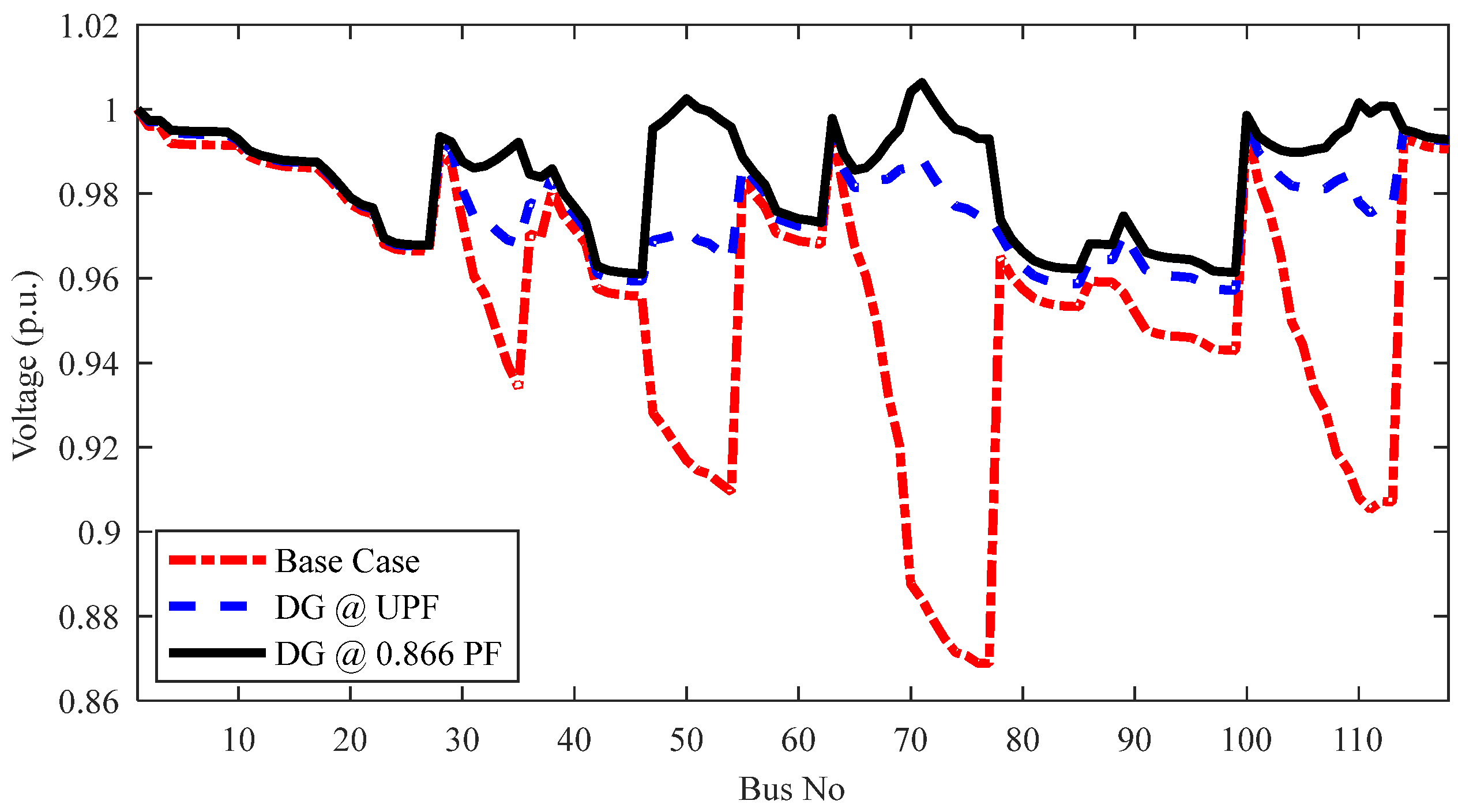
5.2. Test System 2 (118 Bus)

Test system 2 is a 118 bus, [41] large-scale distribution network that caters to total real and reactive power loads of 22,710 kW and 170,410 kVAr, respectively. A voltage and power base of 11 kV and 100 MVA are chosen for the test system.

5.2.1. Scenario I

In this scenario, the mono-objective function of real power loss minimization is simulated to determine the optimal allocations of the DG units. The results for this scenario for both UPF-DGs (case 1) and 0.866 LPF-DGs (case 2) are compared in

Table 8. Comparison of the results for the real power loss minimization of 118 bus DN.

Case 1: Allocation of UPF-DGs
Methods	Optimal Bus	Optimal DG Size, MW	RPL, kW	VD (p.u.)	RCVSI (p.u.)	CVSI (p.u.)	Worst	Average	Standard Deviation
SCA	71	2.9858	668.3339	0.1025	1.2045	0.8302	711.4617	684.4184	10.2363
	50	3.0869
	109	2.9708
DEA	50	2.7890	668.9599	0.1001	1.2137	0.8239	684.7815	678.0098	4.1155
	71	3.2081
	110	2.8750
O-SCMDEA	50	2.8836	667.2830	0.1038	1.2067	0.8287	668.3581	667.4956	0.2334
	71	2.9785
	109	3.1198
SFSA [52]	71	2.9786	667.29	-	-	-	-	-	-
	109	3.1199
	50	2.8833
Case 2: Allocation of 0.866 LPF-DGs
Methods	Optimal Bus	Optimal DG Size, MW	RPL, kW	VD (p.u.)	RCVSI (p.u.)	CVSI (p.u.)	Worst	Average	Standard Deviation
SCA	71	2.8122	364.5265	0.0581	1.1820	0.8460	418.9182	385.9170	12.4081
	110	3.2202
	50	3.2935
DEA	110	2.8251	370.1841	0.0531	1.1731	0.8524	396.0838	379.8858	5.9381
	50	3.5118
	72	3.1777
O-SCMDEA	71	3.0191	362.7833	0.0552	1.1768	0.8497	364.9054	363.0446	0.4034
	50	3.2795
	110	3.1123

. The results reveal that, for UPF-DGs, the real power loss reduction attained by the proposed method is 667.2830 kW from 1298.1 kW of the base case, which is the minimum as compared to a loss reduction of 668.3339 kW, 668.9599 kW and 667.29 kW attained by the SCA, DEA and SFSA, respectively. The loss reduction by the O-SCMDEA for 0.866 LPF-DGs is 362.7833 kW from 1298.1 kW of the base case, which is also the minimum compared to 364.5265 kW and 370.1841 kW yielded by the SCA and DEA, respectively. Further, the loss reduction obtained by 0.866 LPF-DGs is significantly less than UPF-DGs, which is due to the additional reactive power support received from the lagging power factor operation of the DG units. Moreover, the standard deviation of the results obtained by O-SCMDEA is the lowest compared to the SCA and DEA for both the cases, as can be seen from the 10th column of Table 8. It implies O-SCMDEA is more robust in solving the optimal allocation of the DGs to minimize the real power loss of the distribution network as compared to the SCA and DE. The convergence characteristics of the SCA, DEA and O-SCMDEA for loss reduction for both the cases are portrayed in Figure 8. It confirms the faster convergence of O-SCMDEA on the optimal value compared to SCA and DEA.

5.2.2. Scenario II

This scenario deals with the mono-objective function to improve the voltage profile of the distribution system. A system with a voltage deviation close to zero will have voltages of all nodes close to the substation. For test system 2, the voltage deviation without integration of the DG units is 0.3576 p.u., which can be considered as very poor. Further, several nodes have voltages below 0.95 p.u., and the 77th node experiences the minimum voltage of 0.8688 p.u., as given in Table 2.

Table 9. Comparison of the results for the voltage deviation minimization of 118 bus DN.

Case 1: Allocation of UPF-DGs
Methods	Optimal Bus	Optimal DG Size, MW	RPL, kW	VD (p.u.)	RCVSI (p.u.)	CVSI (p.u.)	Worst	Average	Standard Deviation
SCA	51	4.4391	872.6374	0.0623	1.1807	0.8470	0.0719	0.0657	0.0027
	110	4.3284
	73	4.5226
DEA	113	3.9466	919.0408	0.0623	1.1818	0.8462	0.0726	0.0670	0.0022
	53	4.4626
	71	4.3906
O-SCMDEA	109	4.5420	846.4178	0.0598	1.1799	0.8475	0.0610	0.0603	0.0003
	52	4.5327
	71	4.5420
Case 2: Allocation of 0.866 LPF-DGs
Methods	Optimal Bus	Optimal DG Size, MW	RPL, kW	VD (p.u.)	RCVSI (p.u.)	CVSI (p.u.)	Worst	Average	Standard Deviation
SCA	108	3.5205	402.1593	0.0473	1.1682	0.8560	0.0545	0.0502	0.0021
	48	4.2757
	70	3.6499
DEA	49	4.2750	417.6226	0.0483	1.1682	0.8560	0.0523	0.0499	0.0013
	109	4.2741
	70	3.7444
O-SCMDEA	109	3.5587	480.7784	0.0458	1.1665	0.8572	0.0472	0.0465	0.0003
	47	4.5419
	69	4.5420

depicts the results obtained by different methods in solving the optimal DG allocation for voltage profile improvement for scenario II. It shows that the voltage deviation of the test system as obtained by O-SCMDEA is 0.0598 p.u. and 0.0458 p.u. for UPF-DGs and 0.866 LPF-DGs, respectively. It means that DGs operating at lagging power factor have a significant impact in maintaining a better voltage profile than those working at UPF. Moreover, the standard deviation of the results obtained by O-SCMDEA is the lowest compared to the SCA and DEA for both the cases, as can be seen from the 10th column of Table 9. It suggests that O-SCMDEA is more robust in solving the optimal DG allocation to maintain the near-flat voltage operation of the distribution network. A comparison of the convergence characteristics of the SCA, DEA and O-SCMDEA for scenario II is shown in Figure 9. Undoubtedly, O-SCMDEA performs the best in finding the global optima compared to the SCA and DEA.

5.2.3. Scenario III

In this scenario, the optimal DG allocation is solved to minimize the mono-objective function of RCVSI. Table 2 reflects that this test system has a base case RCVSI of 1.7552 p.u., which is too high and can increase the risk of a more catastrophic voltage collapse.

Table 10. Comparison of the results for the RCVSI minimization of 118 bus DN.

Case 1: Allocation of UPF-DGs
Methods	Optimal Bus	Optimal DG Size, MW	RPL, kW	VD (p.u.)	RCVSI (p.u.)	CVSI (p.u.)	Worst	Average	Standard Deviation
SCA	71	4.5127	791.5745	0.0743	1.1801	0.8474	1.1895	1.1837	0.0028
	52	4.1823
	110	2.3826
DEA	73	4.5297	887.3179	0.0691	1.1806	0.8470	1.1865	1.1827	0.0017
	107	4.1548
	53	4.0613
O-SCMDEA	70	4.5420	813.3903	0.0620	1.1799	0.8475	1.1799	1.1799	0.0000
	111	4.1298
	50	4.4931
Case 2: Allocation of 0.866 LPF-DGs
Methods	Optimal Bus	Optimal DG Size/pf, MW	RPL, kW	VD (p.u.)	RCVSI (p.u.)	CVSI (p.u.)	Worst	Average	Standard Deviation
SCA	69	4.2171	491.1881	0.0574	1.1667	0.8571	1.1713	1.1680	0.0013
	50	4.5155
	109	2.5253
DEA	75	4.0919	532.5343	0.0645	1.1666	0.8572	1.1687	1.1674	0.0006
	35	4.5372
	113	2.9958
O-SCMDEA	71	3.8966	418.3989	0.0483	1.1665	0.8572	1.1665	1.1665	0.0000
	47	4.5420
	110	3.7129

presents the results reported by the SCA, DEA and O-SCMDEA for both cases of scenario III. The RCVSI obtained by O-SCMDEA is 1.1799 p.u. and 1.1665 p.u. for case 1 and case 2, respectively, which is the minimum compared to the results obtained by that of the SCA and DEA, as presented in the 6th column of Table 10. Once again, the optimal allocation of 0.866 LPF-DGs has shown to have a better RCVSI than UPF-DGs. It conveys that the lagging power factor of DGs can save the system from possible voltage collapse by providing additional VAR support. Further, O-SCMDEA has provided a better solution for optimal DG allocation to reduce the RCVSI compared to the other methods, as reported in Table 10. Moreover, the standard deviation of the results obtained by O-SCMDEA is small for both the cases compared to that of the SCA and DE, making it a more robust algorithm to handle the optimal DG allocation for scenario III. Figure 10 displays the convergence characteristics of the SCA, DEA and O-SCMDEA for scenario III. It claims a faster and near-optimal convergence O-SCMDEA compared to the SCA and DEA.

5.2.4. Scenario IV

In this scenario, the simultaneous play among the IRPL, IVDI and IIVSI in deciding the optimal DG allocation is envisaged by combining them through suitable weights to form a weighted sum multi-objective function.

Table 11. Comparison of the results for the simultaneous optimization of the RPL, VD and RCVSI of 118 bus DN.

	Case 1: Allocation of UPF-DGs
Methods	Optimal Bus	Optimal DG Size, MW	RPL, kW	VD (p.u.)	RCVSI (p.u.)	CVSI (p.u.)	Best	Worst	Average	Standard Deviation
SCA	72	3.5674	688.6312	0.0829	1.1950	0.8369	0.8023	0.8596	0.8173	0.0129
	50	3.4299
	109	3.2648
DEA	50	3.2784	700.4404	0.0792	1.1878	0.8419	0.8010	0.8255	0.8115	0.0067
	110	3.3129
	71	4.0025
O-SCMDEA	50	3.6013	693.8726	0.0789	1.1914	0.8394	0.7976	0.7987	0.7979	0.0004
	109	3.5000
	71	3.7778
Case 2: Allocation of 0.866 LPF-DGs
Methods	Optimal Bus	Optimal DG Size, MW	RPL, kW	VD (p.u.)	RCVSI (p.u.)	CVSI (p.u.)	Best	Worst	Average	Standard Deviation
SCA	49	3.6552	382.2600	0.0493	1.1722	0.8531	0.4968	0.5400	0.5146	0.0129
	71	3.6823
	110	3.2913
DEA	109	3.6156	377.8895	0.0502	1.1722	0.8531	0.4948	0.5201	0.5047	0.0060
	50	3.6505
	72	3.3616
O-SCMDEA	110	3.1823	367.2104	0.0508	1.1724	0.8530	0.4877	0.4896	0.4881	0.0005
	71	3.2768
	50	3.6255

compares the values of real power loss, voltage deviation and RCVSI as obtained by different methods for the optimal allocation for both types of DGs to minimize the multi-objective function. For case 1, the power loss yielded by O-SCMDEA is 693.8726 kW, which is slightly higher than 688.6312 kW obtained by the SCA and much better than 700.4404 kW as achieved by the DEA. In terms of improvement in VD, the results obtained by O-SCMDEA outperform that of the SCA and DEA for case 1. For RCVSI, the DEA gives marginally better results than that of O-SCMDEA. However, a look at the 10th column of Table 11 reveals that the overall performance of the proposed method in optimizing the multi-objective function is superlative as compared to the SCA and DEA. Similarly, for case 2, O-SCMDEA evolves as a clear-cut winner so far as minimization of the real power loss and multi-objective function is concerned. However, the results achieved by O-SCMDEA for case 2 fall marginally short in terms of the VD and RCVSI from the SCA and DEA, respectively. Once again, the standard deviation of the results obtained by O-SCMDEA is far better than that of the SCA and DEA for both cases of the DG operation. Therefore, O-SCMDEA qualifies as a more robust algorithm for large-scale test systems to handle the optimal DG allocation. Further, the comparison of the convergence characteristic of the SCA, DEA and O-SCMDEA as depicted in Figure 11 reveals that the proposed method has a faster convergence on the near-global optima. The voltage profile and branch current profile of the test system for both cases of scenario IV are depicted in Figure 12 and Figure 13, respectively. The performance of the test system is found to be better both in terms of a better voltage profile and much-reduced feeder currents for 0.866 LPF-DG units than UPF-DGs and no DGs, respectively.

5.3. Test System 3 (136 Bus)

Test system 3 is a 136 bus [48] large-scale distribution network that caters to total real and reactive power loads of 18,314 kW and 7932.5 kVAr, respectively. A voltage and power base of 13.8 kV and 100 MVA are chosen for the test system.

5.3.1. Scenario I

This scenario deals with the results of the proposed algorithm in minimizing the mono-objective function of real power loss UPF-DGs (case 1) and 0.866 LPF-DGs (case 2), respectively.

Table 12. Comparison of the results for real power loss minimization of 136 bus DN.

Case 1: Allocation of UPF-DGs
Methods	Optimal Bus	Optimal DG Size, MW	RPL, kW	VD (p.u.)	RCVSI (p.u.)	CVSI (p.u.)	Worst	Average	Standard Deviation
SCA	106	2.6695	169.9215	0.0561	1.1683	0.8559	182.0513	173.3227	2.5778
	52	2.2958
	14	2.1442
DEA	106	2.4656	170.8067	0.0578	1.1788	0.8483	176.8662	172.9326	1.5905
	32	2.0684
	11	2.1037
O-SCMDEA	11	2.3138	169.0198	0.0543	1.1644	0.8588	170.0238	169.3736	0.2329
	106	2.7471
	29	2.0813
SFSA [52]	11	2.3284	169.22	-	-	-	-	-	-
	29	2.0639
	106	2.8411
Case 2: Allocation of 0.866 LPF-DGs
Methods	Optimal Bus	Optimal DG Size, MW	RPL, kW	VD (p.u.)	RCVSI (p.u.)	CVSI (p.u.)	Worst	Average	Standard Deviation
SCA	28	1.9321	145.1953	0.0314	1.1247	0.8892	157.5103	149.7313	2.5098
	14	1.9132
	106	2.5198
DEA	11	1.9540	144.8097	0.0315	1.1247	0.8892	151.7665	148.6051	1.6503
	106	2.7060
	28	1.9279
O-SCMDEA	29	1.9853	144.3359	0.0314	1.1247	0.8892	145.7097	144.7496	0.3791
	11	2.1430
	106	2.6509

lists the results achieved by the SCA, DEA, O-SCMDEA and SFSA for minimizing the real power loss for both cases. The real power loss is reduced from 320.35 kW to 169.9215 kW, 170.8067 kW, 169.0198 kW and 169.22 kW by the SCA, DEA, O-SCMDEA and SFSA, respectively, for case 1. Similarly, for case 2, the real power loss reduction achieved by the SCA, DEA and O-SCMDEA is 145.1953 kW, 144.8097 kW and 144.3359 kW, respectively. Hence, the proposed method is found to be effective in solving DG allocation for real power loss minimization compared to the rest of the established algorithms listed in Table 12. Moreover, a better loss reduction reported for optimal 0.866 LPF-DGs is considered than UPF-DGs. The standard deviation of the results listed in the 10th column of Table 12 confirms that the proposed method is more robust in handling large-scale test systems. The comparative convergence characteristics of the SCA, DEA and O-SCMDEA for both cases of scenario I are depicted in Figure 14.

5.3.2. Scenario II

This scenario deals with the mono-objective function to improve the voltage profile of the distribution system.

Table 13. Comparison of the results for the voltage deviation minimization of 136 bus DN.

Case 1: Allocation of UPF-DGs
Methods	Optimal Bus	Optimal DG Size, MW	RPL, kW	VD (p.u.)	RCVSI (p.u.)	CVSI (p.u.)	Worst	Average	Standard Deviation
SCA	112	2.5454	313.3257	0.0428	1.1247	0.8892	0.0458	0.0436	0.0008
	139	2.4247
	39	2.6735
DEA	108	2.5399	292.4590	0.0427	1.1247	0.8892	0.0435	0.0431	0.0002
	109	2.3667
	36	2.7387
O-SCMDEA	107	2.7471	317.7009	0.0422	1.1247	0.8892	0.0426	0.0423	0.0001
	35	2.7471
	111	2.7459
Case 2: Allocation of 0.866 LPF-DGs
Methods	Optimal Bus	Optimal DG Size, MW	RPL, kW	VD (p.u.)	RCVSI (p.u.)	CVSI (p.u.)	Worst	Average	Standard Deviation
SCA	32	2.1588	156.1567	0.0306	1.1247	0.8892	0.0310	0.0307	0.0001
	53	1.9880
	107	2.3991
DEA	33	1.9622	156.6345	0.0305	1.1247	0.8892	0.0307	0.0306	0.0001
	107	2.4224
	49	2.1238
O-SCMDEA	107	2.4250	155.5813	0.0305	1.1247	0.8892	0.0305	0.0305	0.0000
	28	2.0162
	52	2.0359

depicts the results obtained by different methods in solving the optimal DG allocation for voltage profile improvement for scenario II. It shows that the voltage deviation of the test system as obtained by O-SCMDEA is 0.0422 p.u. and 0.0305 p.u. for UPF-DGs and 0.866 LPF-DGs, respectively. It means that DGs operating at a lagging power factor have a significant impact in maintaining a better voltage profile than those operating at UPF. Moreover, the standard deviation of the results obtained by O-SCMDEA is the lowest compared to the SCA and DEA for both the cases, as can be seen from the 10th column of Table 13. It suggests that O-SCMDEA is more robust in solving optimal DG allocation to maintain the near-flat voltage operation of the distribution network. A comparison of the convergence characteristics of the SCA, DEA and O-SCMDEA for scenario II is shown in Figure 15. Undoubtedly, O-SCMDEA performs the best in finding the global optima compared to SCA and DEA.

5.3.3. Scenario III

In this scenario, the optimal DG allocation is solved to minimize the mono-objective function of the reciprocal of the RCVSI.

Table 14. Comparison of the results for the RCVSI minimization of 136 bus DN.

Case 1: Allocation of UPF-DGs
Methods	Optimal Bus	Optimal DG Size, MW	RPL, kW	VD (p.u.)	RCVSI (p.u.)	CVSI (p.u.)	Worst	Average	Standard Deviation
SCA	83	2.5450	282.6227	0.0507	1.1244	0.8894	1.1244	1.1244	0.0000
	116	1.3566
	107	2.6755
DEA	105	2.0635	240.5822	0.0526	1.1244	0.8894	1.1244	1.1244	0.0000
	80	2.6144
	107	2.4912
O-SCMDEA	105	1.7622	241.6850	0.0582	1.1244	0.8894	1.1244	1.1244	0.0000
	108	2.3341
	76	2.7160
Case 2: Allocation of 0.866 LPF-DGs
Methods	Optimal Bus	Optimal DG Size, MW	RPL, kW	VD (p.u.)	RCVSI (p.u.)	CVSI (p.u.)	Worst	Average	Standard Deviation
SCA	107	2.0087	218.5893	0.0459	1.1163	0.8958	1.1163	1.1163	0.0000
	07	1.4092
	84	2.6585
DEA	78	2.1711	239.5010	0.0491	1.1163	0.8958	1.1163	1.1163	0.0000
	02	0.9261
	114	1.6455
O-SCMDEA	09	1.3358	212.7348	0.0445	1.1163	0.8958	1.1163	1.1163	0.0000
	112	1.9140
	85	2.2992

presents the results reported by the SCA, DEA and O-SCMDEA for both cases of scenario III. The RCVSI obtained by O-SCMDEA is 1.1244 p.u. and 1.1163 p.u. for case 1 and case 2, respectively, which is identically the same as obtained by the SCA and DEA, as presented in the 6th column of Table 14. Once again, the optimal allocation of the lagging DGs was shown to have a better RCVSI than UPF-DGs. Moreover, the standard deviation of the results obtained by all the methods listed in Table 14 is zero, which implies that all of them are equally capable of handling the optimal DG allocation for scenario III. Figure 16 displays the convergence characteristics of the SCA, DE and O-SCMDEA for both cases of scenario III.

5.3.4. Scenario IV

In this scenario, the simultaneous optimization of the IRPL, IVD and IIVSI is considered for deciding the optimal DG allocation in the framework of a weighted sum multi-objective function.

Table 15. Comparison of the results for the simultaneous optimization of the RPL, VD and RCVSI of 136 bus DN.

Case 1: Allocation of UPF-DGs
Methods	Optimal Bus	Optimal DG Size, MW	RPL, kW	VD (p.u.)	RCVSI (p.u.)	CVSI (p.u.)	Best	Worst	Average	Standard Deviation
SCA	28	2.4913	177.2554	0.0500	1.1374	0.8792	0.9749	1.0299	1.0063	0.0135
	111	2.7243
	14	1.8872
DEA	16	2.0078	176.6420	0.0505	1.1361	0.8802	0.9741	0.9979	0.9837	0.0066
	127	2.3062
	108	2.7415
O-SCMDEA	108	2.7471	174.6281	0.0489	1.1358	0.8805	0.9594	0.9663	0.9630	0.0022
	11	2.5168
	29	2.3742
Case 2: Allocation of 0.866 LPF-DGs
Methods	Optimal Bus	Optimal DG Size, MW	RPL, kW	VD (p.u.)	RCVSI (p.u.)	CVSI (p.u.)	Best	Worst	Average	Standard Deviation
SCA	14	1.8750	145.0432	0.0314	1.1247	0.8892	0.7668	0.8213	0.7906	0.0145
	106	2.5911
	29	1.9050
DEA	29	1.9134	146.2388	0.0316	1.1247	0.8892	0.7715	0.7917	0.7777	0.0059
	106	2.4123
	09	2.1102
O-SCMDEA	106	2.6099	144.3639	0.0314	1.1247	0.8892	0.7645	0.7687	0.7664	0.0013
	11	2.1151
	29	1.9888

compares the values of different objectives as obtained by other methods for the optimal allocation of both UPF-DGs and 0.866 LPF-DGs of scenario IV. For case 1, the values of the RPL, VD and RCVSI attained by O-SCMDEA are 174.6281 kW, 0.0489 p.u. and 1.1358 p.u., respectively, which are the lowest as compared to that of the SCA and DEA. Similarly, the values of the RPL, VD and RCVSI attained by O-SCMDEA are 144.3639 kW, 0.0314 p.u. and 1.1247 p.u., respectively, which are the lowest compared to the SCA and DEA for case 2. Therefore, O-SCMDEA qualifies as a more robust algorithm for large-scale test systems to handle the optimal DG allocation. Further, the comparison of the convergence characteristics of the SCA, DEA and O-SCMDEA as depicted in Figure 17 reveals that the proposed method has a faster convergence on the near-global optima. The voltage profile and branch current profile of the test system for both cases of scenario IV are depicted in Figure 18 and Figure 19, respectively. The performance of the test system is found to be better both in terms of a better voltage profile and a much-reduced feeder current for the optimal allocation of 0.866 LPF-DGs than UPF-DGs and no DGs, respectively.

5.4. Statistical Analysis

To establish the superiority of the proposed method, optimal allocation of the DG units for real power loss minimization (considering both DG types) was solved for 50 independent trial runs of the SCA, DEA and O-SCMDEA. Box plots for scenario 1, by all the three methods across the three test systems, are compared in Figure 20, Figure 21 and Figure 22, respectively. A box plot provides a visual description of datasets in five distinct ranges: minimum, first quartile, median, third quartile and maximum range. A box is drawn connecting the first and third quartiles and spreads over the interquartile range of 2σ, where σ represents the standard deviation of the dataset. The median value of the data is represented by the horizontal line drawn within the box. The vertical lines connecting the first quartile to a minimum value of the data and the third quartile to the maximum data value are called whiskers. The minimum and maximum ranges of the dataset are represented by plus marks and called outliers. A lower σ value is evident for the proposed technique across all the test systems for scenario I. It implies that O-SCMDEA is more robust than the SCA and DEA in solving the optimal DG allocation even for the larger test systems. Further, the comparison of the statistical features in Table 4 with O-SCMDEA corresponding to case 1 and case 2 of Scenario I for the 33 bus system of the QOCSOS algorithm (as reported in Reference [21] for 30 independent trial runs) also proves the robustness of the proposed method.

Normality tests reveal whether the data are drawn from a normal distribution or not. Therefore, in this work, the Shapiro–Wilk test and Kolmogorov–Smirnov test were performed for a normality check, and the results are presented in

Table 16. Normality test for O-SCMDEA for scenario I applied to the different test systems.

Test Systems	p-Values at 5% Significance Level
	Shapiro–Wilk Test		Kolmogorov–Smirnov Test
	Case 1	Case 2	Case 1	Case 2
33 bus	2.0326 × 10−6	3.0820 × 10−8	1.74 × 10−45	1.74 × 10−45
118 bus	1.5110 × 10−6	2.5179 × 10−8	1.74 × 10−45	1.74 × 10−45
136 bus	1.0532 × 10−4	3.7513 × 10−4	1.74 × 10−45	1.74 × 10−45

. The table shows that the p-values obtained by both tests across the three test systems are less than the assumed significance level of 5%. Hence, it can be said with a 95% confidence level that the results obtained by the proposed method are not drawn from any normal distribution.

Further, the Friedman–ANOVA and Wilcoxon signed-rank tests, which are standard nonparametric tests, were also performed for the post hoc analysis, and the results are presented in

Table 17. Friedman–ANOVA test of O-SCMDEA for scenario I applied to the different test systems.

Test Systems	Methods
	SCA		DEA		O-SCMDEA
	Case 1	Case 2	Case 1	Case 2	Case 1	Case 2
33 bus	1.1374	0.9705	0.3145	0.4340	0.0571	0.0700
118 bus	10.2363	12.4081	4.1155	5.9381	0.2334	0.4034
136 bus	2.5778	2.5098	1.5905	1.6503	0.2329	0.3791

and

Table 18. Wilcoxon signed-rank test for scenario I applied to the different test systems.

Test Systems	Methods
	OSCMDE Versus SCA		OSCMDE Versus DEA
	Case 1	Case 2	Case 1	Case 2
33 bus	5.3181 × 10−17	1.8392 × 10−17	3.7392 × 10−17	5.0155 × 10−17
118 bus	7.5041 × 10−18	7.5041 × 10−18	7.0661 × 10−18	7.0661 × 10−18
136 bus	7.5041 × 10−18	1.2120 × 10−17	7.0661 × 10−18	1.9517 × 10−17

, respectively. In Table 16, the lower p-values of the proposed technique for both cases of scenario I across the three test systems as compared to the other methods prove its superiority. Pairwise comparisons of the p-values for the different algorithms are shown in Table 17. The p-values less than the significance level of 5% suggest that the differences in the mean values of the results obtained by different techniques are of statistical significance.

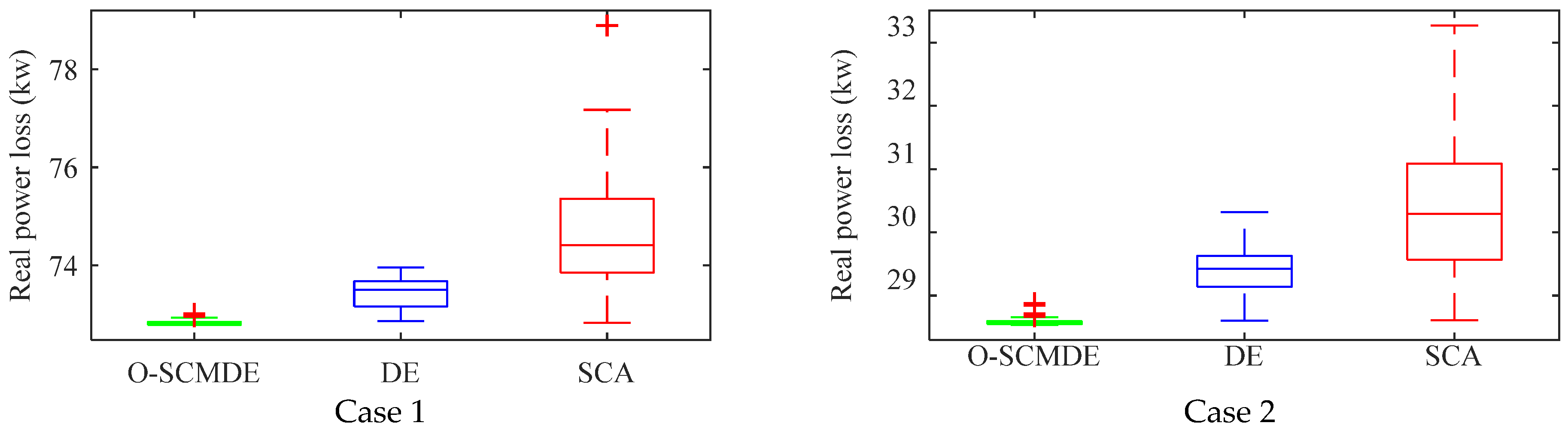
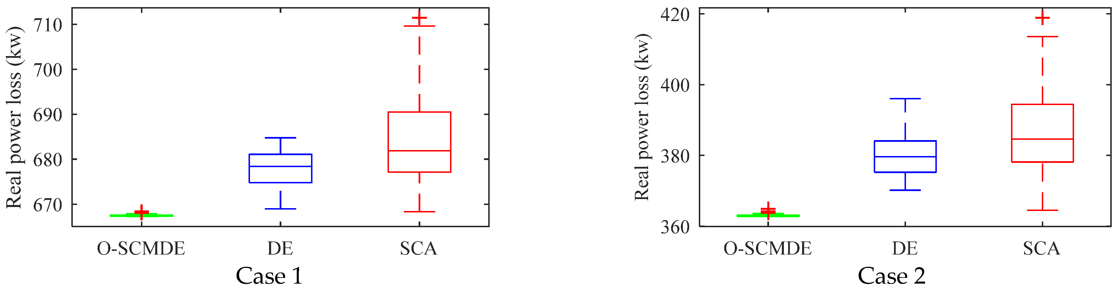
5.5. Solution Quality

The results obtained by the proposed O-SCMDEA for solving the OADG for all the studied test systems are compared with state-of-the-art metaheuristic approaches in Table 4, Table 5, Table 6, Table 7, Table 8, Table 9, Table 10, Table 11, Table 12, Table 13, Table 14 and Table 15. It can be seen that the best results obtained by O-SCMDEA are the lowest as compared to all the reported metaheuristic approaches for all scenarios across all the studied test systems. Additionally, for the larger test systems (118 bus and 136 bus), the solutions provided by the O-SCMDEA are considerably better as compared to those of the SCA, DEA and SFSA [51]. Hence, it confirms that the proposed method provides a high-quality solution for solving the OADG.

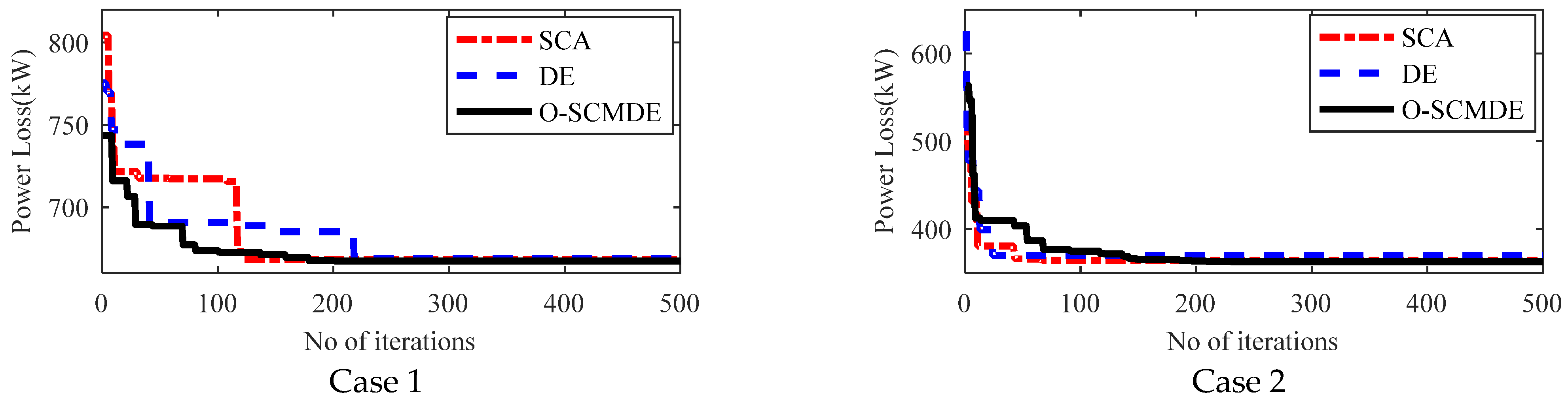
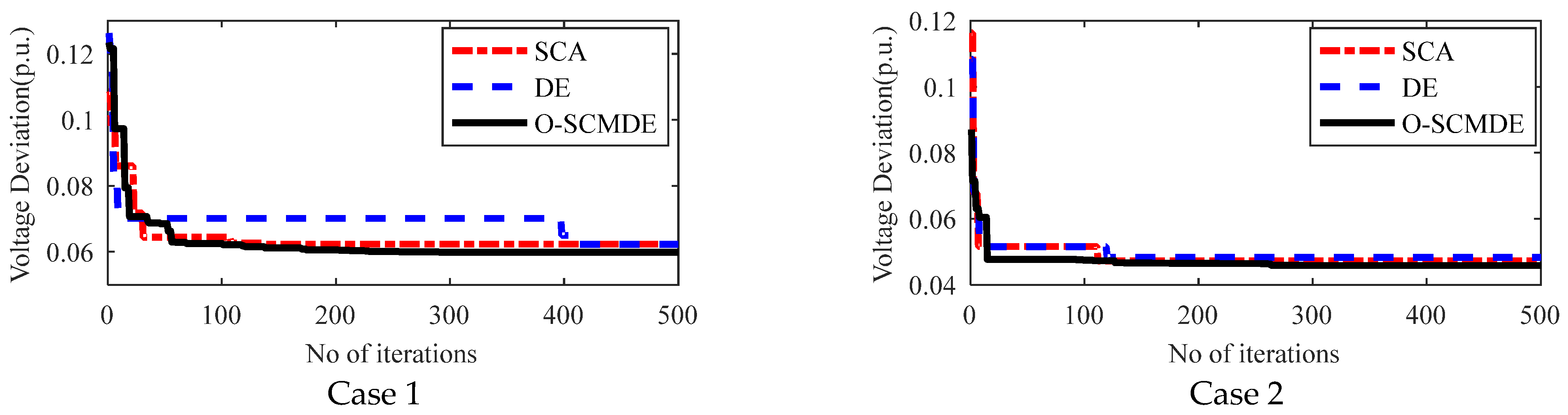
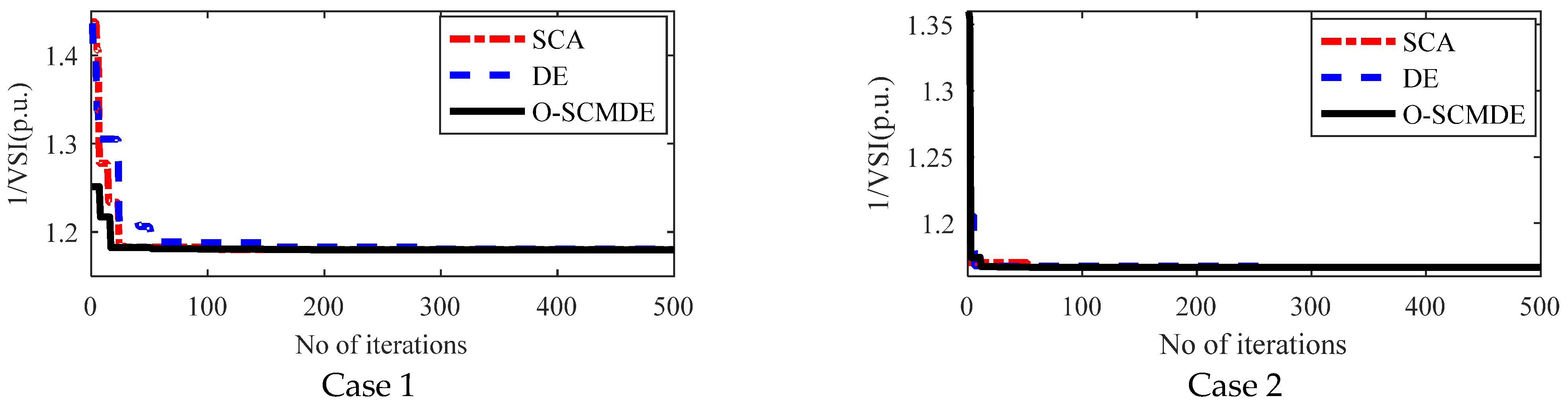
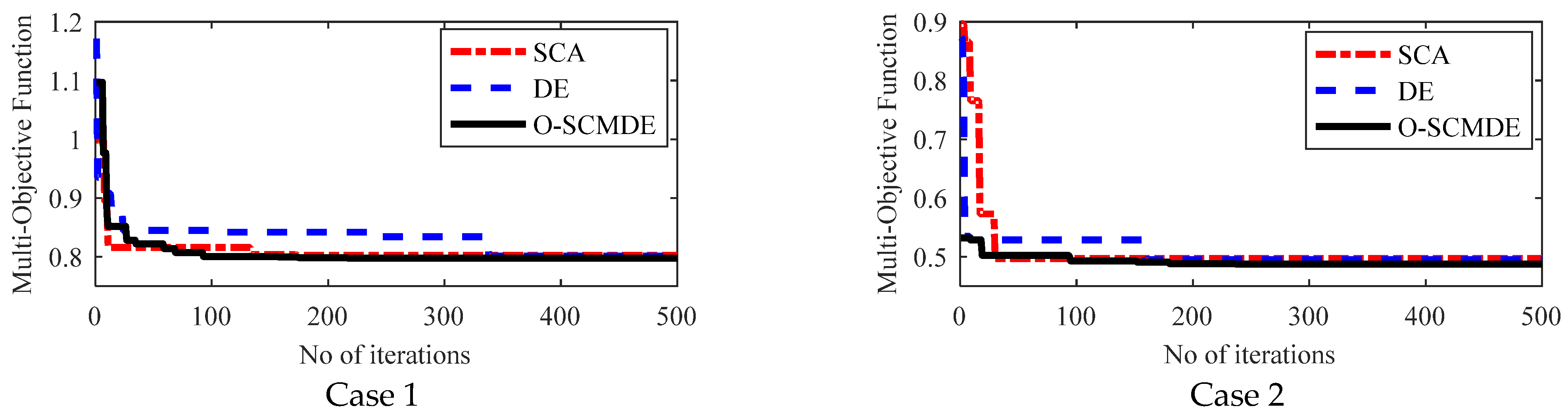
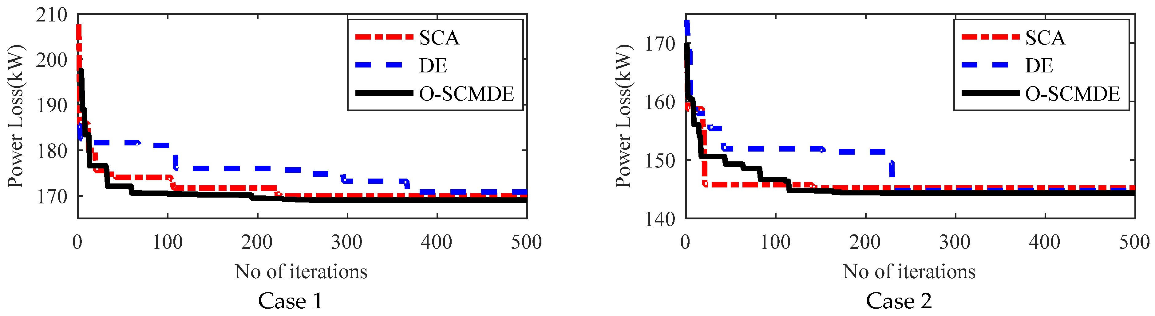
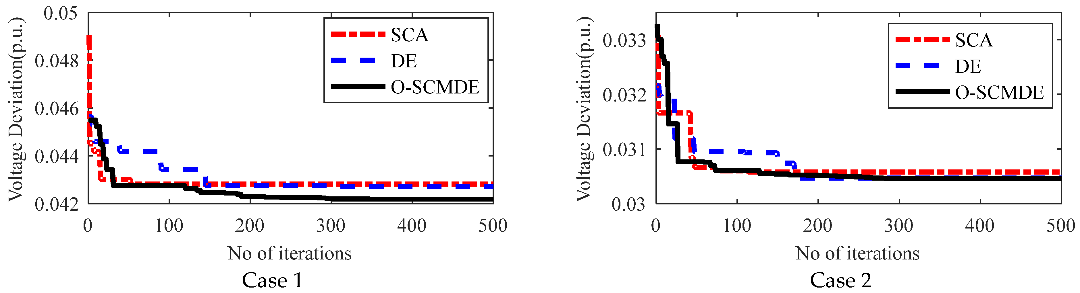
5.6. Convergence Charecteristics

The convergence characteristics of the proposed O-SCMDEA algorithm are compared with those of the SCA and DEA in their respective convergence characteristic figures for all the test systems. All these figures illustrate that O-SCMDEA reaches the near-optimal solution faster than the SCA and DEA. This faster convergence accounts for the adoption of the oppositional learning and hybridization of the SCA and DEA, which effectively balances the search space’s exploration and exploitation, respectively.

5.7. Computational Time

For completeness, the computational time of the proposed O-SCMDE and studied SCA and DEA for solving the OADG are compared in

Table 19. Comparison of the simulation time for Scenario I applied to the studied test systems.

Test Systems	Methods
	SCA		DEA		O-SCMDEA
	Case 1	Case 2	Case 1	Case 2	Case 1	Case 2
33 bus	4.1963 s	4.0840 s	7.6427 s	7.4453 s	11.2348 s	10.9250 s
118 bus	14.0647 s	13.7444 s	27.4197 s	27.2257 s	39.7063 s	38.3187 s
136 bus	21.4209 s	21.3897 s	42.0096 s	39.1550 s	63.6492 s	56.9987 s

. For this purpose, the above algorithms were simulated for one trial run considering a fixed population size of 50 and maximum iterations of 100 for all test systems for the minimization of the real power loss only. From Table 19, it can be seen that the SCA is the fastest, whereas the proposed O-SCMDEA is the slowest in solving the OADG. Due to the joint execution of both the SCA and DEA, O-SCMDEA took more execution time than both of them. However, in terms of robustness, convergence characteristics and solution quality, O-SCMDEA outperforms the SCA, DEA and other reported metaheuristic approaches.

6. Conclusions

The inherent advantage of hybridizing two complementing metaheuristic methods, namely the SCA and DEA, has been utilized to propose a new O-SCMDEA algorithm. Opposition-based learning has also been strategically incorporated to improve the convergence speed and evade stagnation. The algorithm has been effectively implemented for the OADG problem in three test distribution networks (33, 118 and 136 buses) considering four scenarios (three separate mono-objectives of power loss minimization, voltage deviation minimization and maximization of VSIc and a multi-objective framework for all three objectives in combination). For each of the mentioned scenarios, OADG was solved for the optimal allocation of UPF-DGs and LPF-DGs (0.95 lagging for 33 bus and 0.866 lagging for 118 bus and 136 bus). It has been established through the detailed analysis of the results that the proposed hybrid algorithm has superior performance in terms of attainment of the individual objectives and the multi-objective formulation, including the convergence characteristics compared to the SCA and DEA algorithms. The results of O-SCMDEA for solving the OADG were also compared with the recent metaheuristic approaches, such as the QOCSOS, WCA, SFSA and OTCDE, which further confirms the supremacy of the proposed method for solving the OADG, especially for large-scale distribution networks. Box plots were presented for Scenario 1 of all the test systems in the statistical analysis section, confirming the moderately better robustness of the proposed method than the SCA and DEA. The Shapiro–Wilk test and Kolmogorov–Smirnov test were performed for a normality check considering both DG types in each of the three test distribution systems, leading to confirmation of non-generation of the results drawn from any normal distribution. The Friedman–ANOVA and Wilcoxon signed-rank tests were also performed for a post hoc analysis of both cases of scenario I across the three test systems compared to the other methods, proving its superiority. It can also be concluded that O-SCMDE outperforms the SCA and DEA in terms of the convergence characteristics and solution quality but with an increased simulation time. In future works, the application of the proposed method can be extended to other planning problems [53,54].

References

1. Willis, H.L. Analytical methods and rules of thumb for modeling DG-distribution interaction. In Proceedings of the IEEE PES Summer Meeting, Seattle, WA, USA, 16–20 July 2000; pp. 1643–1644. [Google Scholar] [CrossRef]
2. Wang, C.; Nehrir, M. Analytical approaches for optimal placement of distributed generation sources in power systems. IEEE Trans. Power Syst. 2004, 19, 2068–2076. [Google Scholar] [CrossRef]
3. Acharya, N.; Mahat, P.; Mithulananthan, N. An analytical approach for DG allocation in primary distribution network. Int. J. Electr. Power Energy Syst. 2006, 28, 669–678. [Google Scholar] [CrossRef]
4. Hung, D.Q.; Mithulananthan, N.; Bansal, R. Analytical Expressions for DG Allocation in Primary Distribution Networks. IEEE Trans. Energy Convers. 2010, 25, 814–820. [Google Scholar] [CrossRef]
5. Aman, M.; Jasmon, G.; Mokhlis, H.; Bakar, A. Optimal placement and sizing of a DG based on a new power stability index and line losses. Int. J. Electr. Power Energy Syst. 2012, 43, 1296–1304. [Google Scholar] [CrossRef]
6. Hung, D.Q.; Mithulanathan, N. Multiple Distributed Generator Placement in Primary Distribution Network for Loss Reduction. IEEE Trans. Ind. Electron. 2013, 60, 1700–1708. [Google Scholar] [CrossRef]
7. Kayal, P.; Chanda, S.; Chanda, C.K. An analytical approach for allocation and sizing of distributed generations in radial distribution network. Int. Trans. Electr. Energy Syst. 2017, 27, e2322. [Google Scholar] [CrossRef]
8. Mahmoud, K.; Yorino, N.; Ahmed, A. Optimal Distributed Generation Allocation in Distribution Systems for Loss Minimization. IEEE Trans. Power Syst. 2016, 31, 960–969. [Google Scholar] [CrossRef]
9. Karunarathne, E.; Pasupuleti, J.; Ekanayake, J.; Almeida, D. The Optimal Placement and Sizing of Distributed Generation in an Active Distribution Network with Several Soft Open Points. Energies 2021, 14, 1084. [Google Scholar] [CrossRef]
10. Diaaeldin, I.; Aleem, S.A.; El-Rafei, A.; Abdelaziz, A.; Zobaa, A.F. Optimal Network Reconfiguration in Active Distribution Networks with Soft Open Points and Distributed Generation. Energies 2019, 12, 4172. [Google Scholar] [CrossRef] [Green Version]
11. Sultana, S.; Roy, P. Multi-objective quasi-oppositional teaching learning based optimization for optimal location of distributed generator in radial distribution systems. Int. J. Electr. Power Energy Syst. 2014, 63, 534–545. [Google Scholar] [CrossRef]
12. Abdelaziz, A.Y.; Hegazy, Y.G.; El-Khattam, W.; Othman, M.M. Optimal Planning of Distributed Generators in Distribution Networks Using Modified Firefly Method. Electr. Power Compon. Syst. 2015, 43, 320–333. [Google Scholar] [CrossRef]
13. Sultana, S.; Roy, P.K. Krill herd algorithm for optimal location of distributed generator in radial distribution system. Appl. Soft Comput. J. 2016, 40, 391–404. [Google Scholar] [CrossRef]
14. Saha, S.; Mukherjee, V. Optimal placement and sizing of DGs in RDS using chaos embedded SOS algorithm. IET Gener. Transm. Distrib. 2016, 10, 3671–3680. [Google Scholar] [CrossRef]
15. Sharma, S.; Bhattacharjee, S.; Bhattacharya, A. Quasi-Oppositional Swine Influenza Model Based Optimization with Quarantine for optimal allocation of DG in radial distribution network. Int. J. Electr. Power Energy Syst. 2016, 74, 348–373. [Google Scholar] [CrossRef]
16. Nguyen, T.P.; Vo, D.N. A novel stochastic fractal search algorithm for optimal allocation of distributed generators in radial distribution systems. Appl. Soft Comput. 2018, 70, 773–796. [Google Scholar] [CrossRef]
17. Jayasree, M.S.; Sreejaya, P.; Bindu, G.R. Multi-Objective Metaheuristic Algorithm for Optimal Distributed Generator Placement and Profit Analysis. Technol. Econ. Smart Grids Sustain. Energy 2019, 4, 1–10. [Google Scholar] [CrossRef] [Green Version]
18. Nematshahi, S.; Rajabi Mashhadi, H. Application of Distribution Locational Marginal Price in optimal simultaneous distributed generation placement and sizing in electricity distribution networks. Int. Trans. Electr. Energy Syst. 2019, 29, e2837. [Google Scholar] [CrossRef]
19. Kumar, S.; Mandal, K.; Chakraborty, N. A novel opposition-based tuned-chaotic differential evolution technique for techno-economic analysis by optimal placement of distributed generation. Eng. Optim. 2019, 52, 303–324. [Google Scholar] [CrossRef]
20. Truong, K.H.; Nallagownden, P.; Elamvazuthi, I.; Vo, D.N. An improved meta-heuristic method to maximize the penetration of distributed generation in radial distribution networks. Neural Comput. Appl. 2020, 32, 10159–10181. [Google Scholar] [CrossRef]
21. Truong, K.H.; Nallagownden, P.; Elamvazuthi, I.; Vo, D.N. A Quasi-Oppositional-Chaotic Symbiotic Organisms Search algorithm for optimal allocation of DG in radial distribution networks. Appl. Soft Comput. 2020, 88, 106067. [Google Scholar] [CrossRef]
22. Selim, A.; Kamel, S.; Jurado, F. Efficient optimization technique for multiple DG allocation in distribution networks. Appl. Soft Comput. 2020, 86, 105938. [Google Scholar] [CrossRef]
23. Hemeida, M.G.; Ibrahim, A.A.; Mohamed, A.A.A.; Alkhalaf, S.; El-Dine, A.M.B. Optimal allocation of distributed generators DG based manta ray based optimization algorithm. Ain Shams Eng. J. 2021, 12, 609–619. [Google Scholar] [CrossRef]
24. Kawambwa, S.; Hamisi, N.; Mafole, P.; Kundaeli, H. A cloud model based symbiotic organism search algorithm for DG allocation in radial distribution network. Evol. Intell. 2021, 15, 545–562. [Google Scholar] [CrossRef]
25. Dash, S.K.; Mishra, S.; Pati, L.R.; Satpathy, P.K. Optimal Allocation of Distributed Generators Using Metaheuristic Algorithms—An Up-to-Date Bibliographic Review. In Green Technology for Smart City and Society; Lecture Notes in Networks and Systems; Sharma, R., Mishra, M., Nayak, J., Naik, B., Pelusi, D., Eds.; Springer: Singapore, 2020; Volume 151, pp. 553–561. [Google Scholar]
26. Prabha, D.R.; Jayabarathi, T. Optimal placement and sizing of multiple distributed generating units in distribution networks by invasive weed optimization algorithm. Ain Shams Eng. J. 2016, 7, 683–694. [Google Scholar] [CrossRef] [Green Version]
27. Ali, M.H.; Mehanna, M.; Othman, E. Optimal planning of RDGs in electrical distribution networks using hybrid SAPSO algorithm. Int. J. Electr. Comput. Eng. IJECE 2020, 10, 6153–6163. [Google Scholar] [CrossRef]
28. Selim, A.; Kamel, S.; Jurado, F. Voltage stability analysis based on optimal placement of multiple DG types using hybrid optimization technique. Int. Trans. Electr. Energy Syst. 2020, 30, e12551. [Google Scholar] [CrossRef]
29. Kansal, S.; Kumar, V.; Tyagi, B. Hybrid approach for optimal placement of multiple DGs of multiple types in distribution networks. Int. J. Electr. Power Energy Syst. 2016, 75, 226–235. [Google Scholar] [CrossRef]
30. Moradi, M.; Abedini, M. A novel method for optimal DG units capacity and location in Microgrids. Int. J. Electr. Power Energy Syst. 2016, 75, 236–244. [Google Scholar] [CrossRef]
31. Suresh, M.; Edward, J.B. A hybrid algorithm based optimal placement of DG units for loss reduction in the distribution system. Appl. Soft Comput. 2020, 91, 106191. [Google Scholar] [CrossRef]
32. Tolba, M.A.; Rezk, H.; Tulsky, V.; Diab, A.A.Z.; Abdelaziz, A.Y.; Vanin, A. Impact of Optimum Allocation of Renewable Distributed Generations on Distribution Networks Based on Different Optimization Algorithms. Energies 2018, 11, 245. [Google Scholar] [CrossRef] [Green Version]
33. Hassan, A.S.; Sun, Y.; Wang, Z. Multi-objective for optimal placement and sizing DG units in reducing loss of power and enhancing voltage profile using BPSO-SLFA. Energy Rep. 2020, 6, 1581–1589. [Google Scholar] [CrossRef]
34. Radosavljevic, J.; Arsic, N.; Milovanovic, M.; Ktena, A. Optimal Placement and Sizing of Renewable Distributed Generation Using Hybrid Metaheuristic Algorithm. J. Mod. Power Syst. Clean Energy 2020, 8, 499–510. [Google Scholar] [CrossRef]
35. Pesaran, M.H.A.; Nazari-Heris, M.; Mohammadi-Ivatloo, B.; Seyedi, H. A hybrid genetic particle swarm optimization for distributed generation allocation in power distribution networks. Energy 2020, 209, 118218. [Google Scholar] [CrossRef]
36. Samala, R.K.; Kotapuri, M.R. Optimal allocation of distributed generations using hybrid technique with fuzzy logic controller radial distribution system. SN Appl. Sci. 2020, 2, 191. [Google Scholar] [CrossRef] [Green Version]
37. Mirjalili, S. SCA: A Sine Cosine Algorithm for solving optimization problems. Knowl. Based Syst. 2016, 96, 120–133. [Google Scholar] [CrossRef]
38. Storn, R.; Price, K. Differential evolution–A simple and efficient heuristic for global optimization over continuous spaces. J. Glob. Optim. 1997, 11, 341–359. [Google Scholar] [CrossRef]
39. Raut, U.; Mishra, S. A new Pareto multi-objective sine cosine algorithm for performance enhancement of radial distribution network by optimal allocation of distributed generators. Evol. Intell. 2020, 14, 1635–1656. [Google Scholar] [CrossRef]
40. Qin, K.; Huang, V.L.; Suganthan, P. Differential Evolution Algorithm with Strategy Adaptation for Global Numerical Optimization. IEEE Trans. Evol. Comput. 2009, 13, 398–417. [Google Scholar] [CrossRef]
41. Mirjalili, S.M.; Mirjalili, S.Z.; Saremi, S.; Mirjalili, S. Sine Cosine Algorithm: Theory, Literature Review, and Application in Designing Bend Photonic Crystal Waveguides. Nat. Inspired Optim. 2019, 811, 201–217. [Google Scholar]
42. Pant, M.; Zaheer, H.; Garcia-Hernandez, L.; Abraham, A. Differential Evolution: A review of more than two decades of research. Eng. Appl. Artif. Intell. 2020, 90, 103479. [Google Scholar] [CrossRef]
43. Nenavath, H.; Jatoth, R.K. Hybridizing sine cosine algorithm with differential evolution for global optimization and object tracking. Appl. Soft Comput. 2018, 62, 1019–1043. [Google Scholar] [CrossRef]
44. Li, Q.; Ning, H.; Gong, J.; Li, X.; Dai, B. A Hybrid Greedy Sine Cosine Algorithm with Differential Evolution for Global Optimization and Cylindricity Error Evaluation. Appl. Artif. Intell. 2020, 35, 171–191. [Google Scholar] [CrossRef]
45. Kumar, S.; Mandal, K.; Chakraborty, N. Optimal DG placement by multi-objective opposition based chaotic differential evolution for techno-economic analysis. Appl. Soft Comput. 2019, 78, 70–83. [Google Scholar] [CrossRef]
46. Nagaballi, S.; Kale, V.S. Pareto optimality and game theory approach for optimal deployment of DG in radial distribution system to improve techno-economic benefits. Appl. Soft Comput. 2020, 92, 106234. [Google Scholar] [CrossRef]
47. Saha, S.; Mukherjee, V. A novel multi-objective chaotic symbiotic organisms search algorithm to solve optimal DG allocation problem in radial distribution system. Int. Trans. Electr. Energy Syst. 2019, 29, e2839. [Google Scholar] [CrossRef]
48. Mishra, S.; Das, D.; Paul, S. A comprehensive review on power distribution network reconfiguration. Energy Syst. 2017, 8, 227–284. [Google Scholar] [CrossRef]
49. Rahnamayan, S.; Tizhoosh, H.; Salama, M.M. Opposition versus randomness in soft computing techniques. Appl. Soft Comput. 2008, 8, 906–918. [Google Scholar] [CrossRef]
50. Mishra, S.; Das, D.; Paul, S. A simple algorithm for distribution system load flow with distributed generation. In Proceedings of the International Conference on Recent Advances and Innovations in Engineering (ICRAIE-2014), Jaipur, India, 9–11 May 2014; IEEE: Piscataway, NJ, USA, 2014; pp. 1–5. [Google Scholar]
51. Latreche, Y.; Mokhlis, H. Optimal Multi-DG Units Incorporation in Distribution Systems using Single and Multi-Objective Approaches based on Water Cycle Algorithm. J. Electr. Syst. 2020, 16, 530–549. [Google Scholar]
52. Tran, T.T.; Truong, K.H.; Vo, D.N. Stochastic fractal search algorithm for reconfiguration of distribution networks with distributed generations. Ain Shams Eng. J. 2020, 11, 389–407. [Google Scholar] [CrossRef]
53. Othman, M.M.; Hegazy, Y.; Abdelaziz, A. Electrical energy management in unbalanced distribution networks using virtual power plant concept. Electr. Power Syst. Res. 2017, 145, 157–165. [Google Scholar] [CrossRef]
54. Shaheen, A.; Elsayed, A.; El-Sehiemy, R.A.; Abdelaziz, A.Y. Equilibrium optimization algorithm for network reconfiguration and distributed generation allocation in power systems. Appl. Soft Comput. 2021, 98, 106867. [Google Scholar] [CrossRef]
Figure 1. Two-bus equivalent of a distribution network.
Energies 15 02267 g001
Figure 2. Comparison of the convergence characteristics of the SCA, DEA and O-SCMDEA for both cases of scenario I of the 33 bus system.
Energies 15 02267 g002
Figure 3. Comparison of the convergence characteristics of the SCA, DEA and O-SCMDEA for both cases of scenario II of the 33 bus system.
Energies 15 02267 g003
Figure 4. Comparison of convergence characteristic of the SCA, DEA and O-SCMDEA for both cases of scenario III of the 33 bus system.
Energies 15 02267 g004
Figure 5. Comparison of the convergence characteristic of the SCA, DEA and O-SCMDEA for both cases of scenario IV of the 33 bus system.
Energies 15 02267 g005
Figure 6. Voltage profile of the 33 bus test system for scenario IV.
Energies 15 02267 g006
Figure 7. Branch current profile of the 33-bus test system for scenario IV.
Energies 15 02267 g007
Figure 8. Comparison of the convergence characteristics of the SCA, DEA and O-SCMDEA for both cases of scenario I of the 118 bus system.
Energies 15 02267 g008
Figure 9. Comparison of the convergence characteristics of the SCA, DEA and O-SCMDEA for both cases of scenario II of the 118 bus system.
Energies 15 02267 g009
Figure 10. Comparison of the convergence characteristics of the SCA, DEA and O-SCMDEA for both cases of scenario III of the 118 bus system.
Energies 15 02267 g010
Figure 11. Comparison of the convergence characteristics of the SCA, DEA and O-SCMDEA for both cases of scenario IV of the 118 bus system.
Energies 15 02267 g011
Figure 12. Voltage profile of the 118 bus test system for scenario IV.
Energies 15 02267 g012
Figure 13. Branch current profile of the 118 bus test system for scenario IV.
Energies 15 02267 g013
Figure 14. Comparison of the convergence characteristics of the SCA, DEA and O-SCMDEA for both cases of scenario I of the 136 bus system.
Energies 15 02267 g014
Figure 15. Comparison of the convergence characteristics of the SCA, DEA and O-SCMDEA for both cases of scenario II of the 136 bus system.
Energies 15 02267 g015
Figure 16. Comparison of the convergence characteristics of the SCA, DEA and O-SCMDEA for both cases of scenario III of the 136 bus system.
Energies 15 02267 g016
Figure 17. Comparison of the convergence characteristics of the SCA, DEA and O-SCMDEA for both cases of scenario IV of the 136 bus system.
Energies 15 02267 g017
Figure 18. Voltage profile of the 136 bus test system for scenario IV.
Energies 15 02267 g018
Figure 19. Branch current profile of the 136 bus test system for scenario IV.
Energies 15 02267 g019
Figure 20. Box plot for scenario I of the 33 bus test system.
Energies 15 02267 g020
Figure 21. Box plot for scenario I of the 118 bus test system.
Energies 15 02267 g021
Figure 22. Box plot for scenario I of the 136 bus test system.
Energies 15 02267 g022