
Fuzzy Logic-Based Load Frequency Control in an Island Hybrid Power System Model Using Artificial Bee Colony Optimization

 ,
,  ,
,  ,
,  ,
,
Abstract
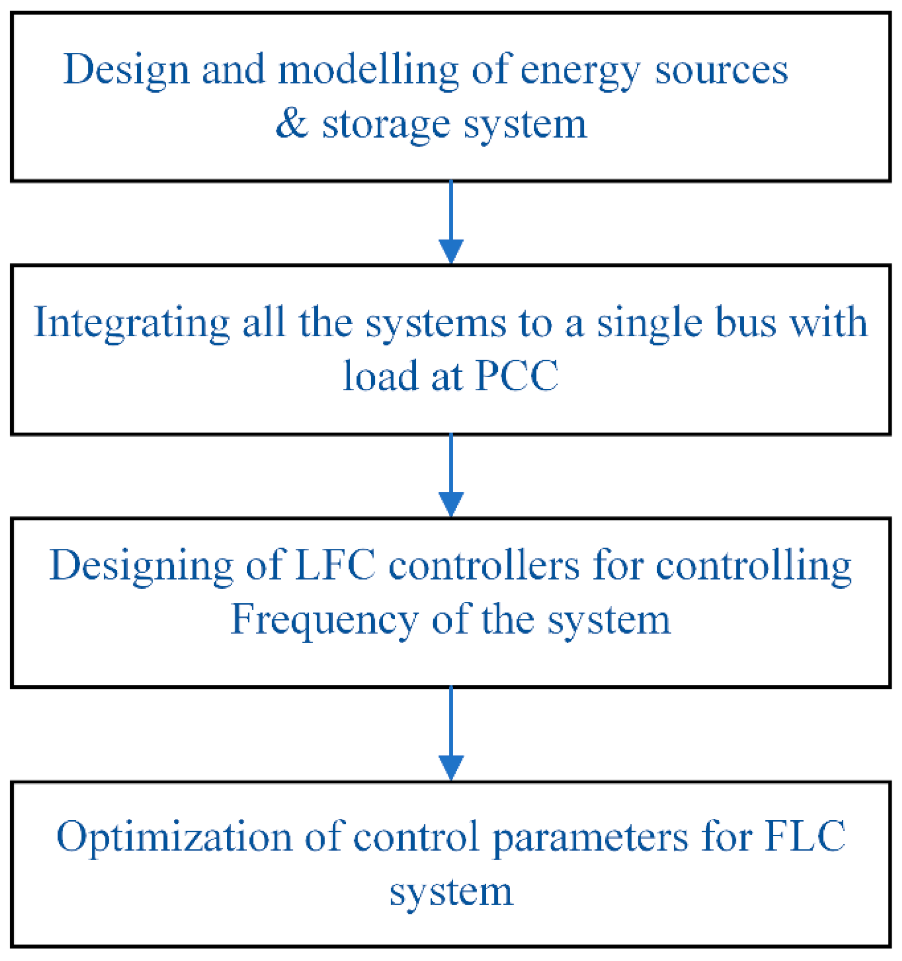
:1. Introduction
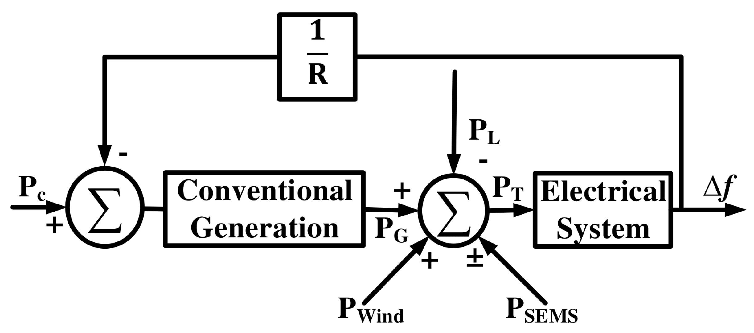
2. System Description
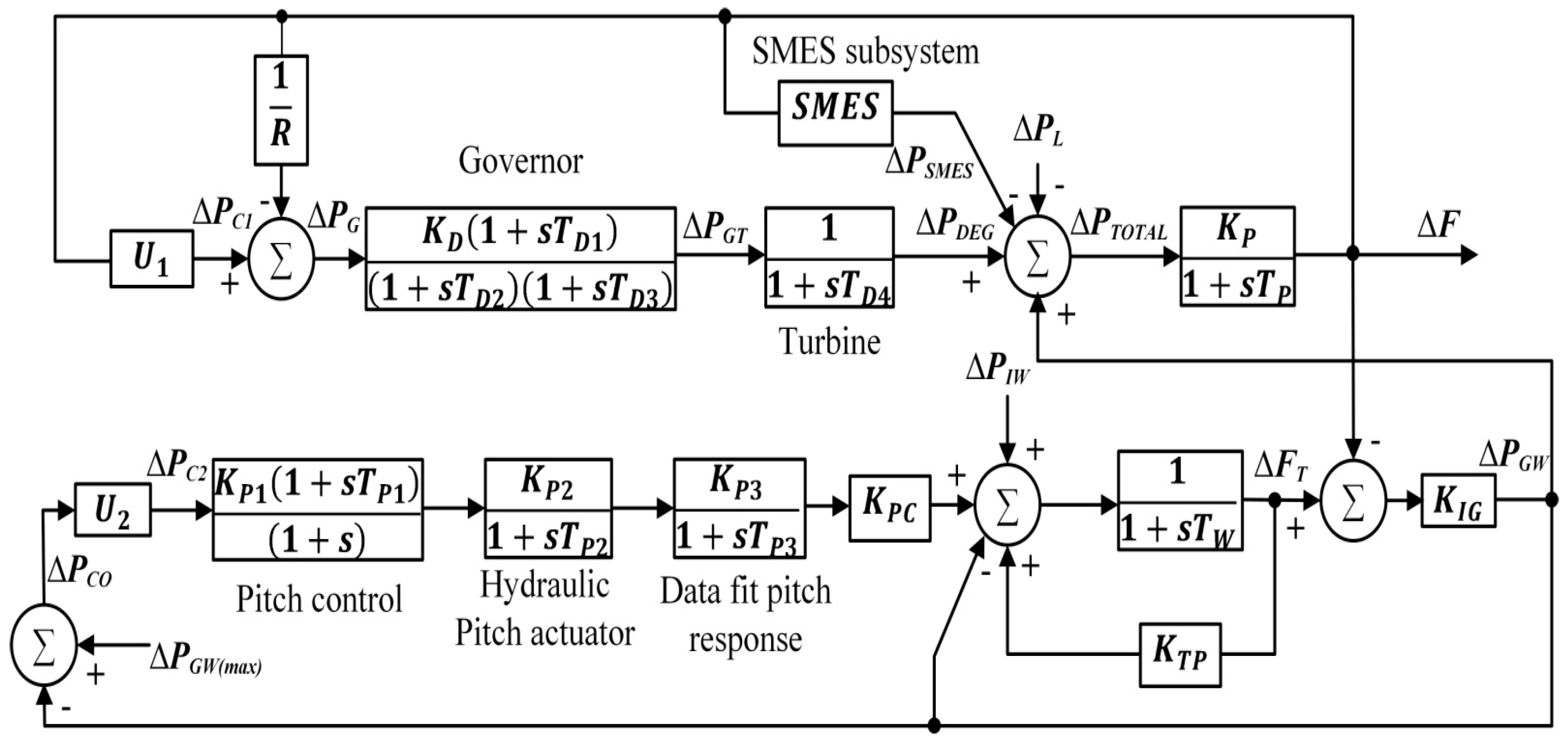
3. System Modelling
3.1. Diesel Generator Model
3.2. Wind Turbine Model
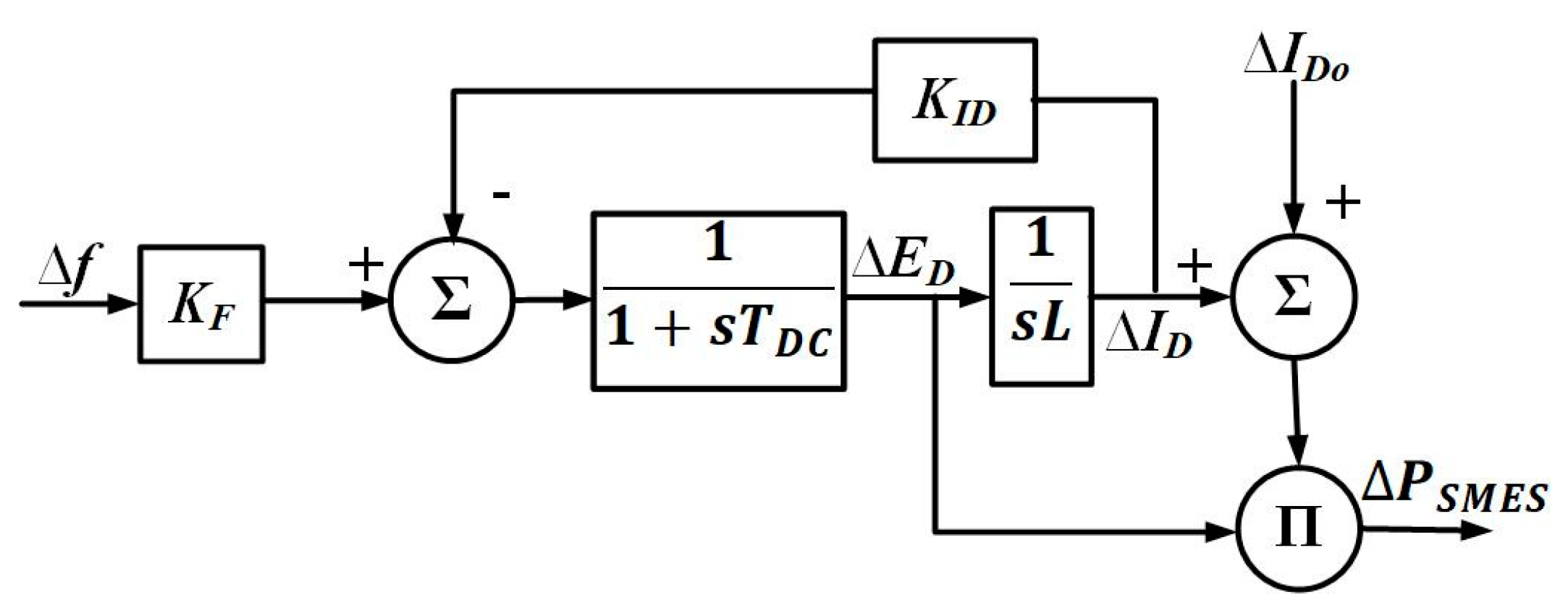
3.3. SMES Model
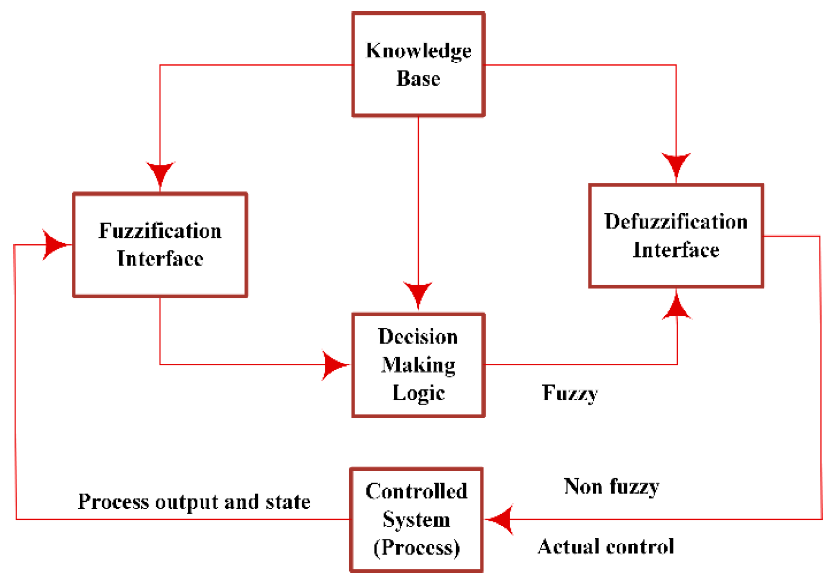
4. Control Methodology
4.1. Classical Controllers
4.1.1. PI Controllers
4.1.2. PD Controllers
4.1.3. PID Controllers
4.2. Performance Parameters
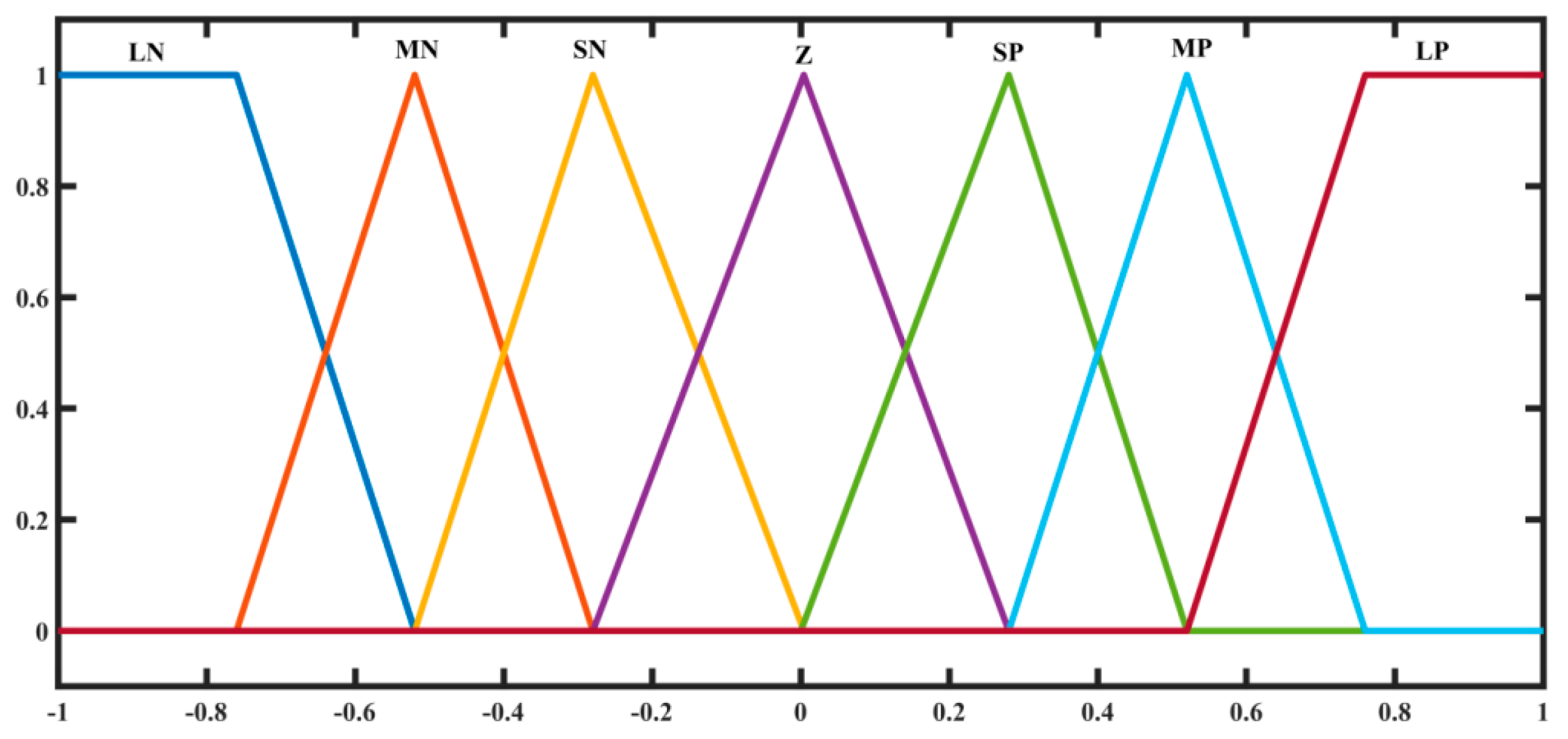
4.3. Design of Intelligent Controllers
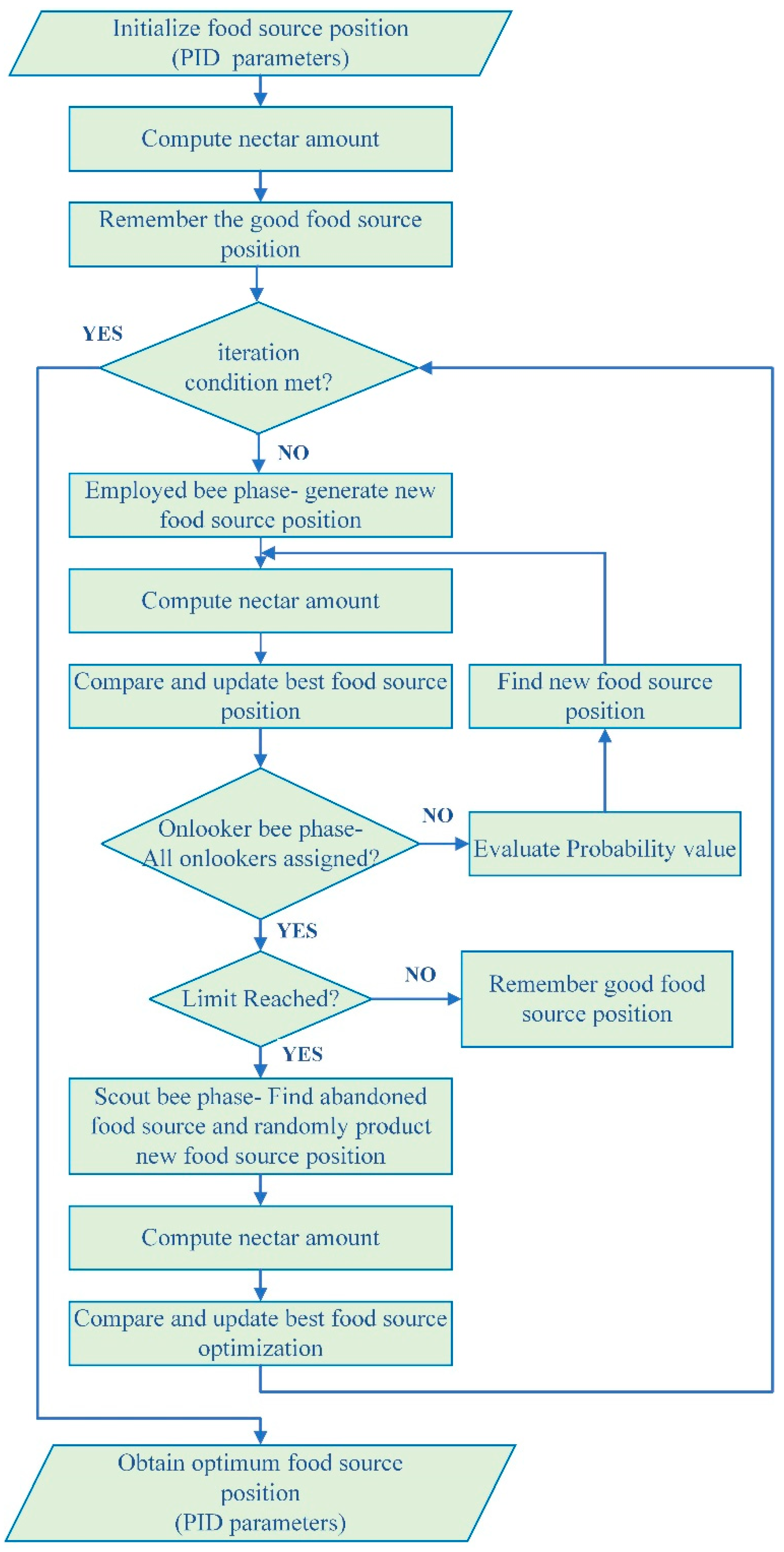
5. Artificial Bee Colony Optimization
- Step1: Set the number of variables, the number of sorts of bees (employers, bystanders, and scooters), and the maximum number of iterations.
- Step2: Produce a random solution for the controller parameters like (23) and (24), where X represents the PID scaling factors for each controller in the system:
- Step3: Calculate the objective function based on (19)
- Step4: Calculate the relative estimation for the hired bees using the formula in (25), where Xi is the cost function for each employed bee based on (19):
- Step5: Create a new food location in the same way as in (26), except that s and t are not identical:
- Step6: Assess the objective function because of the previous criteria: (19).
- Step7: Calculate the probability of obtaining a food source, as in (27):
- Step8: Create a new food source for the observer bees depending on the information provided, as in (27).
- Step9: Check with the scout bees to see if there is a previously used solution.
- Step10: Select the finest solution that has ever been discovered.
- Step11: Has the maximum number of iterations been reached? If this is the case, print the results; otherwise, proceed to step 2.
6. Results and Discussions
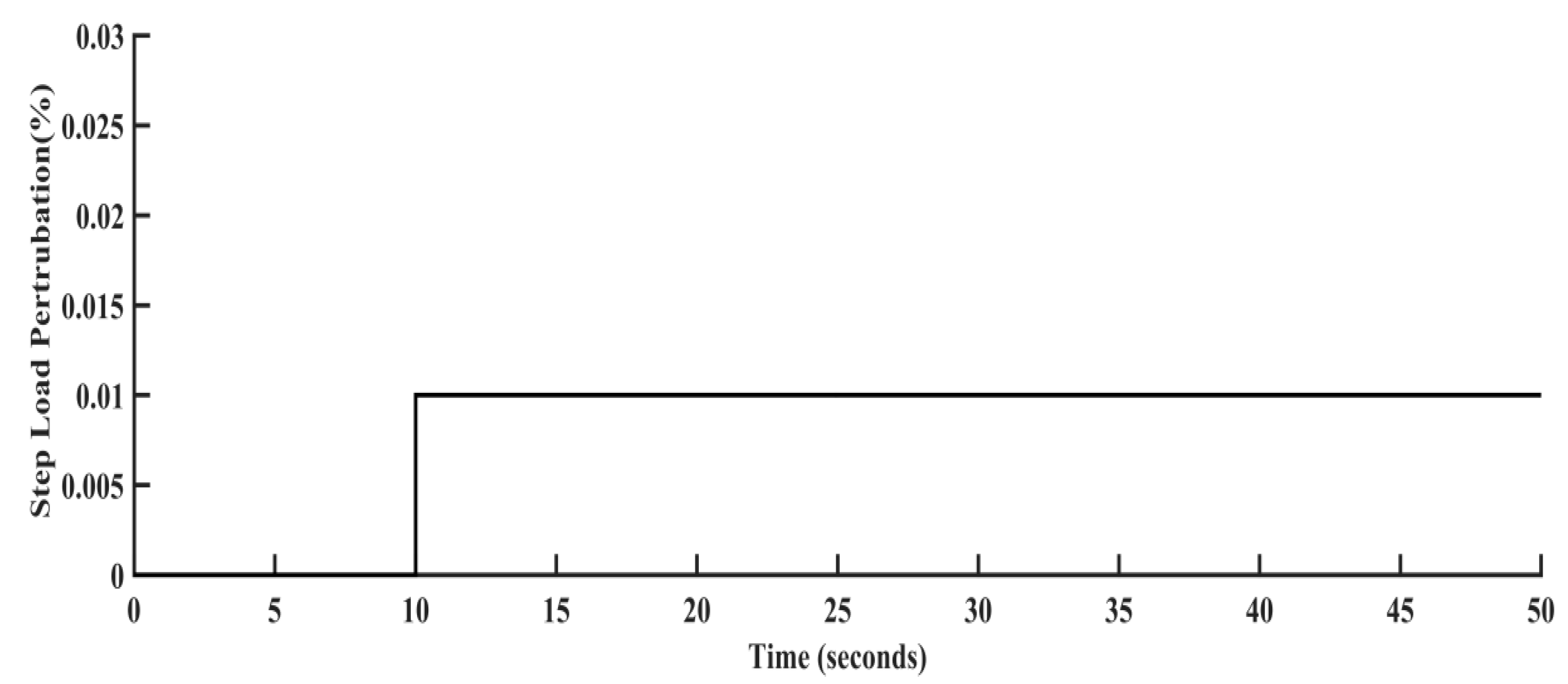
- Case(i) Performance evolution under a 1% raise in step load demand.
- Case(ii) Performance evolution under a 10% and 20% raise in step load demand.
- Case(iii) Performance evolution under random raise in load disturbance.
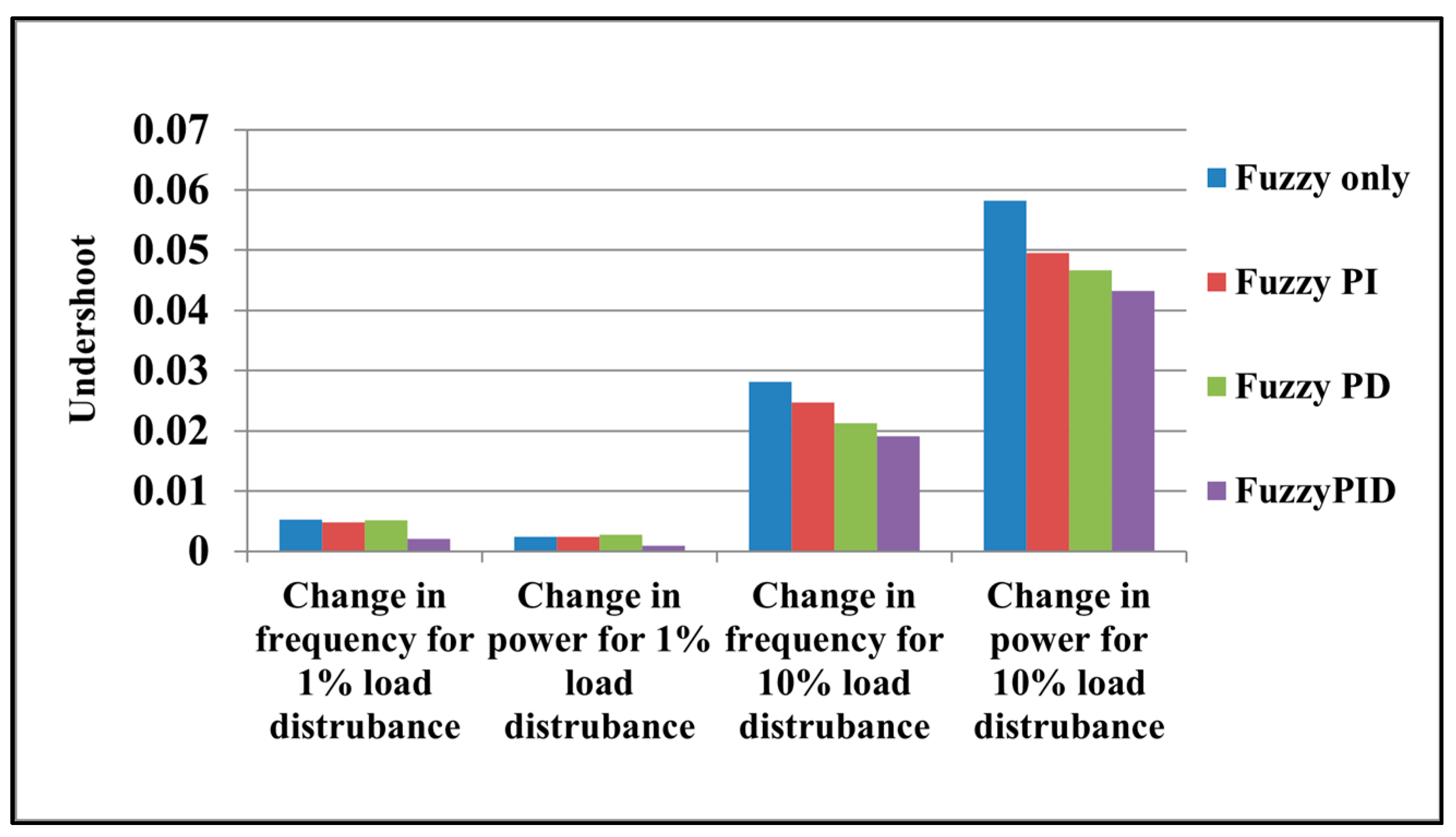
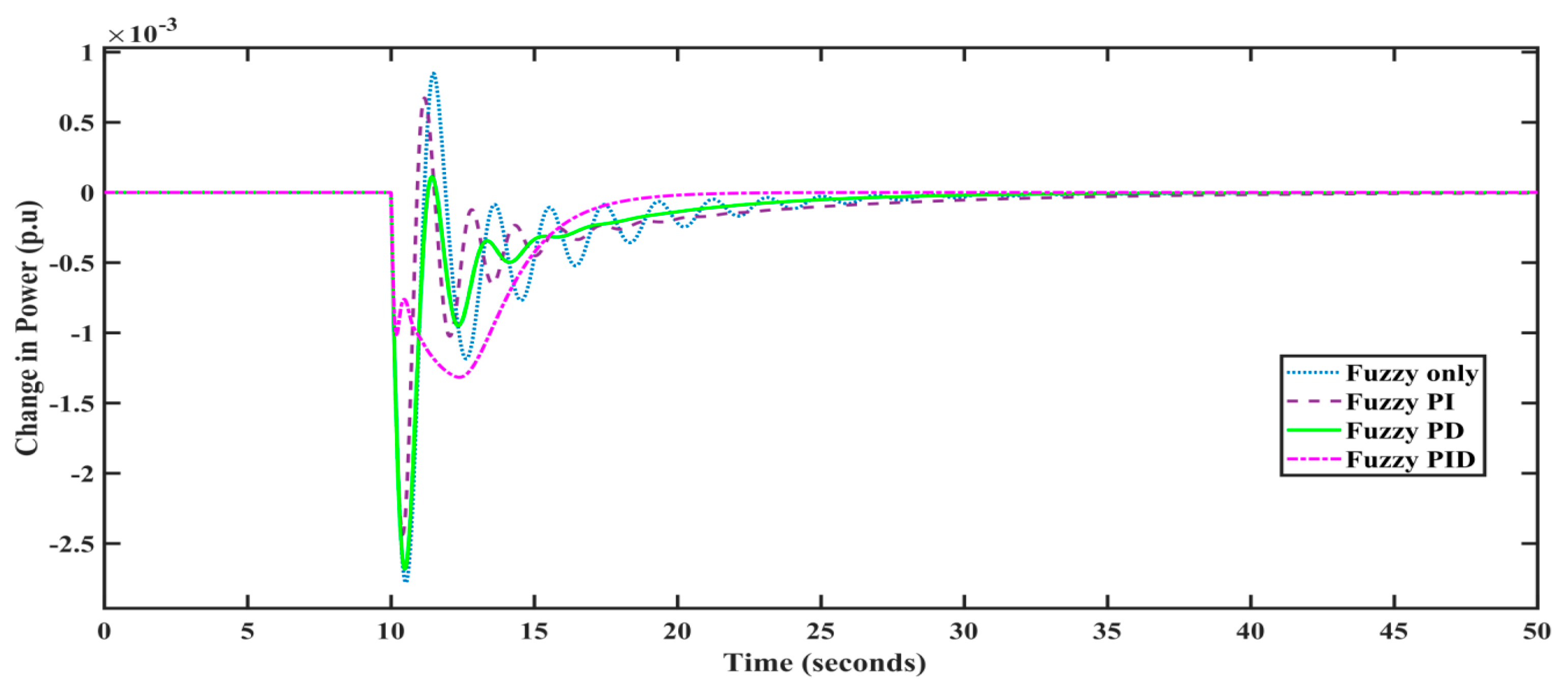
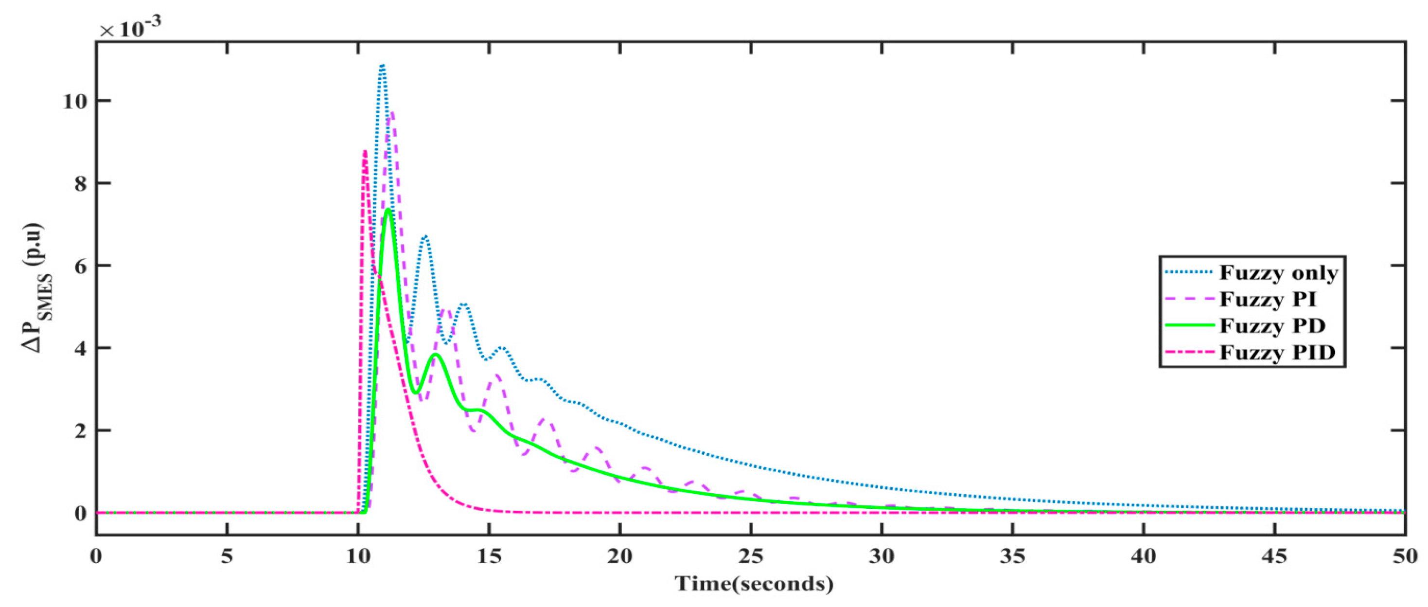
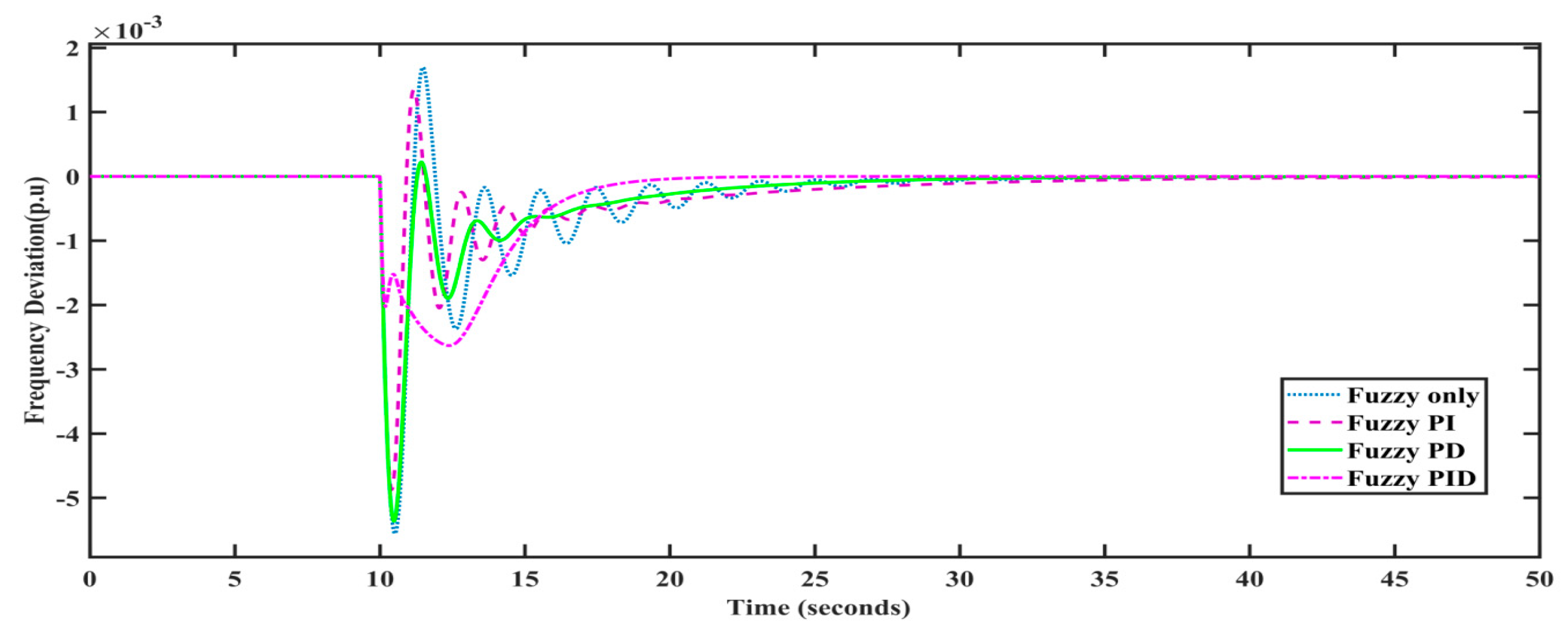
6.1. Case (i) Performance Evolution under a 1% Raise in Step Load Demand
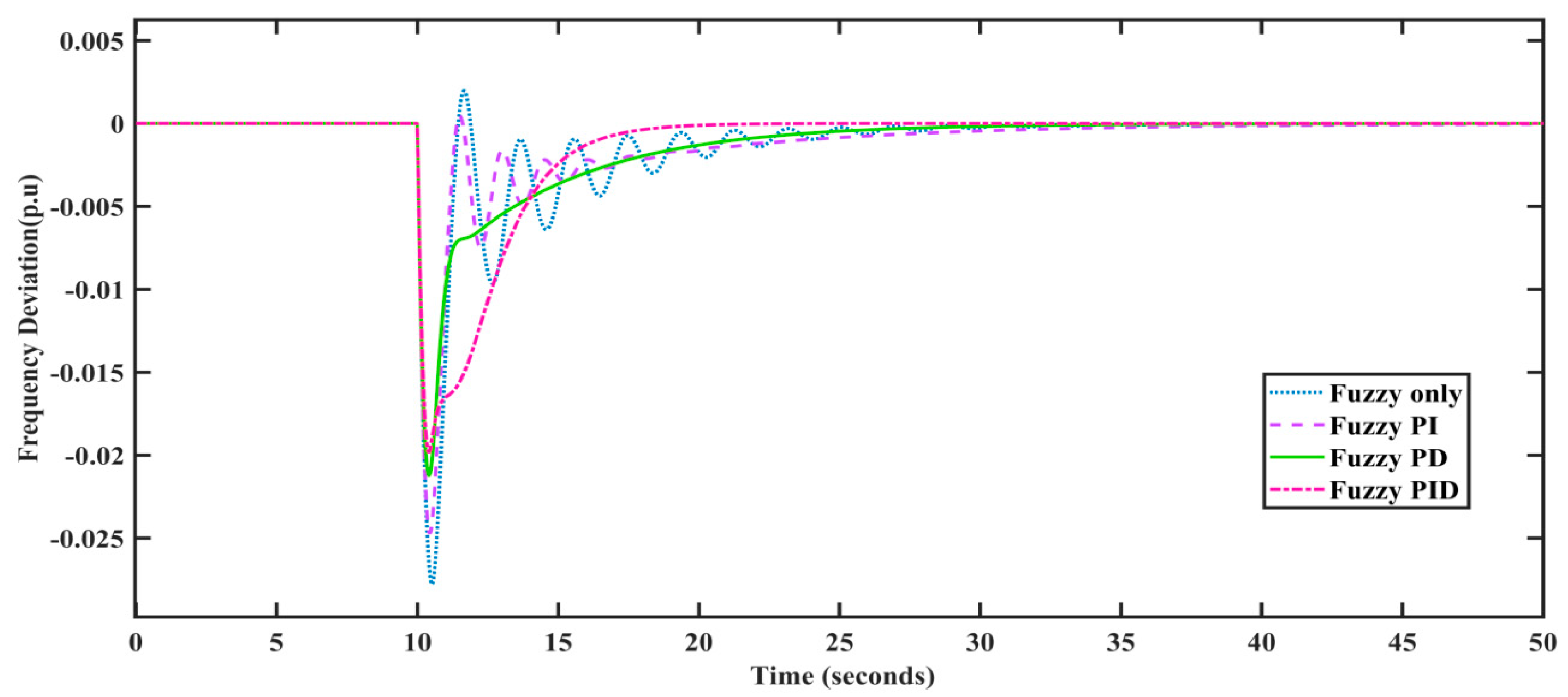
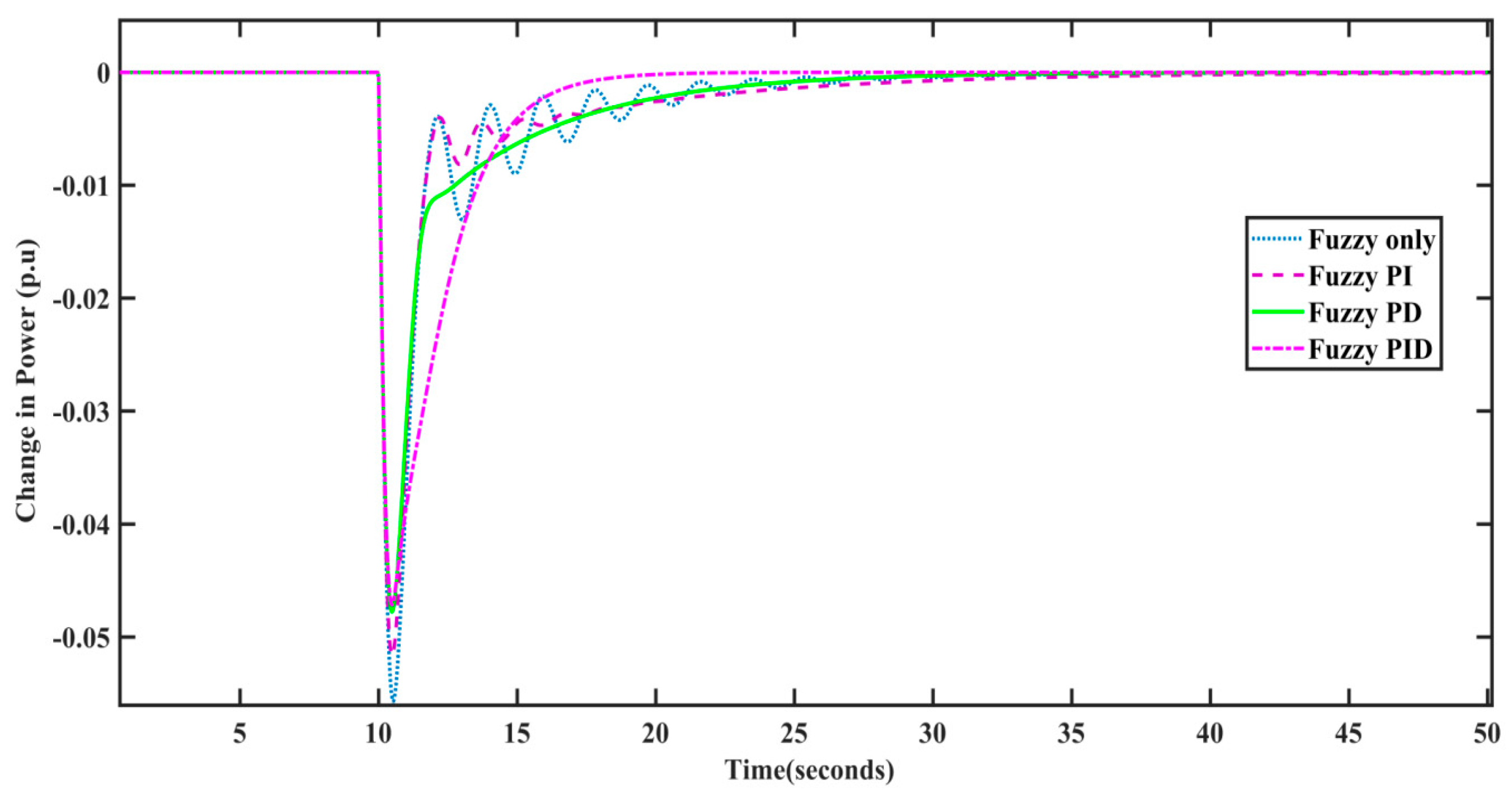
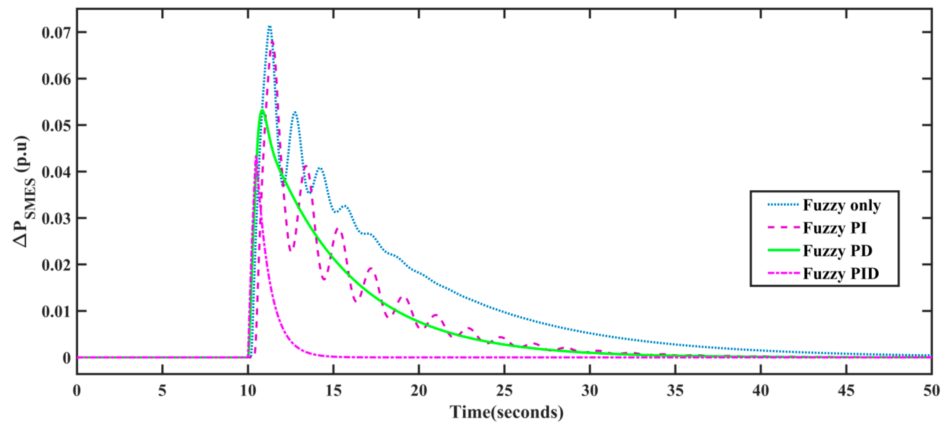
6.2. Case (ii) Performance Evolution under a 10% Raise in Step Load Demand
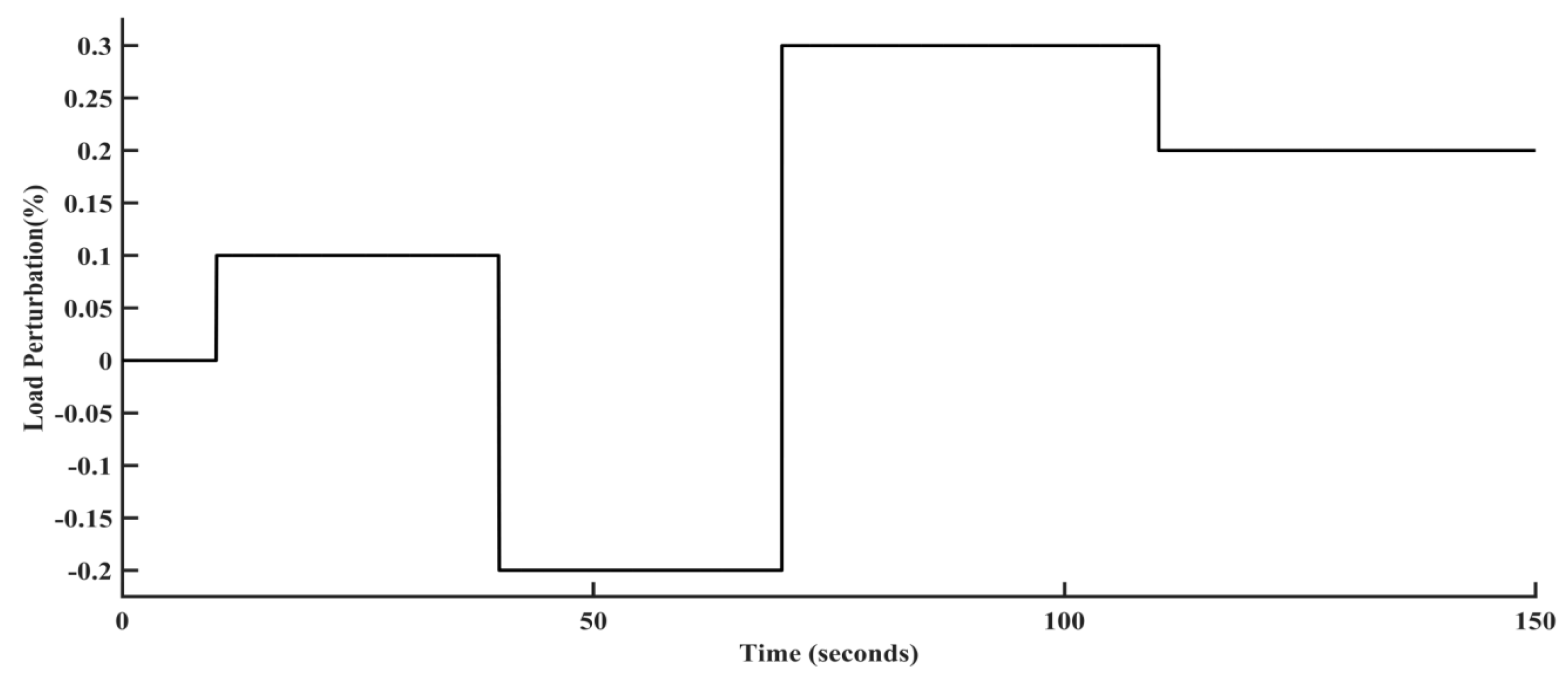
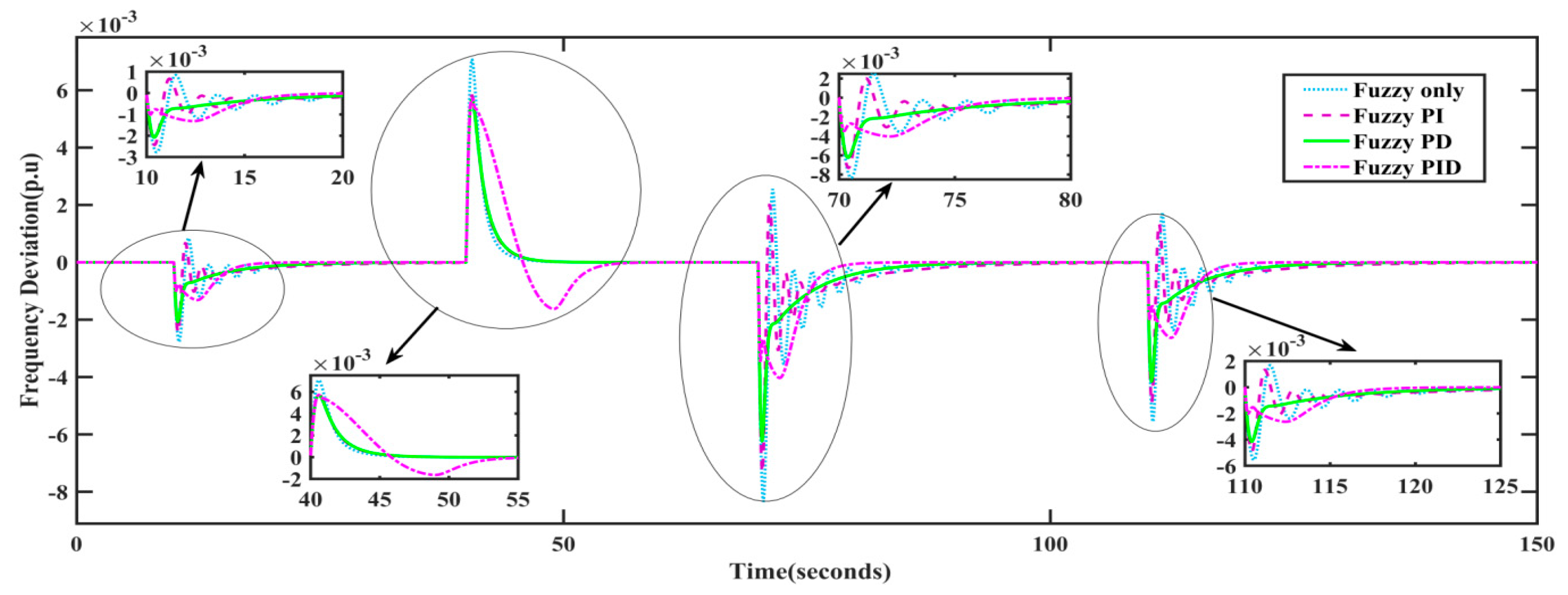
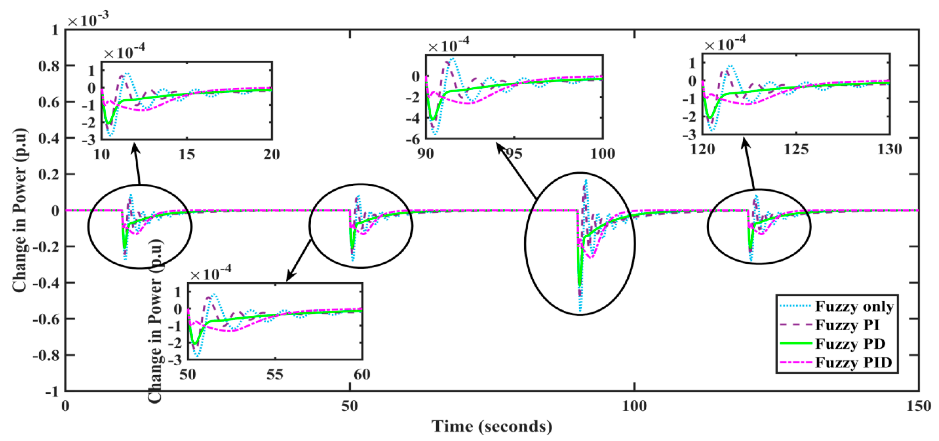
6.3. Case (iii) Performance Evolution under Random Rise in Load Disturbance
7. Conclusions
Author Contributions
Funding
Informed Consent Statement
Conflicts of Interest
References
- He, Y.; Guo, S.; Zhou, J.; Wu, F.; Huang, J.; Pei, H. The quantitative techno-economic comparisons and multi-objective capacity optimization of wind-photovoltaic hybrid power system considering different energy storage technologies. Energy Convers. Manag. 2021, 229, 113779. [Google Scholar] [CrossRef]
- Borenstein, S. The Private and Public Economics of Renewable Electricity Generation. J. Econ. Perspect. 2012, 26, 67–92. [Google Scholar] [CrossRef] [Green Version]
- Gatta, F.M.; Geri, A.; Lauria, S.; Maccioni, M.; Palone, F.; Portoghese, P.; Buono, L.; Necci, A. Replacing diesel generators with hybrid renewable power plants: Giglio smart island project. In Proceedings of the 2017 IEEE International Conference on Environment and Electrical Engineering and 2017 IEEE Industrial and Commercial Power Systems Europe (EEEIC/I&CPS Europe), Milan, Italy, 6–9 June 2017; pp. 1–6. [Google Scholar]
- Abazari, A.; Monsef, H.; Wu, B. Coordination strategies of distributed energy resources including FESS, DEG, FC and WTG in load frequency control (LFC) scheme of hybrid isolated micro-grid. Int. J. Electr. Power Energy Syst. 2019, 109, 535–547. [Google Scholar] [CrossRef]
- Elkadeem, M.R.; Wang, S.; Azmy, A.M.; Atiya, E.G.; Ullah, Z.; Sharshir, S.W. A systematic decision-making approach for planning and assessment of hybrid renewable energy-based microgrid with techno-economic optimization: A case study on an urban community in Egypt. Sustain. Cities Soc. J. 2020, 54, 102013. [Google Scholar] [CrossRef]
- Sebastián, R.; Peña-Alzola, R. Flywheel Energy Storage and Dump Load to Control the Active Power Excess in a Wind Diesel Power System. Energies 2020, 13, 2029. [Google Scholar] [CrossRef] [Green Version]
- Mbungu, N.T.; Naidoo, R.M.; Bansal, R.C.; Siti, M.W.; Tungadio, D.H. An overview of renewable energy resources and grid integration for commercial building applications. J. Energy Storage 2020, 29, 101385. [Google Scholar] [CrossRef]
- Gawas, N.L.; Shengale, R.; Greene, C.M. Quality Analysis of TAT for Supply Restoration Process. In IIE Annual Conference. Proceedings; Institute of Industrial and Systems Engineers: Norcross, GA, USA, 2021; pp. 896–901. [Google Scholar]
- Al-Bahrani, L.T.; Horan, B.; Seyedmahmoudian, M.; Stojcevski, A. Dynamic economic emission dispatch with load dema nd management for the load demand of electric vehicles during crest shaving and valley filling in smart cities environment. Energy 2020, 195, 116946. [Google Scholar] [CrossRef]
- Kumar, K.; Gandhi, V.I. Load frequency control for an isolated hybrid power system with hybrid control technique and comparative analysis with different control techniques. Malay. J. Comput. Sci. 2020, 78–92. [Google Scholar]
- Rajamand, S. Load frequency control and dynamic response improvement using energy storage and modeling of uncertainty in renewable distributed generators. J. Energy Storage 2021, 37, 102467. [Google Scholar] [CrossRef]
- Sitompul, S.; Fujita, G. Impact of Advanced Load-Frequency Control on Optimal Size of Battery Energy Storage in Islanded Microgrid System. Energies 2021, 14, 2213. [Google Scholar] [CrossRef]
- Oshnoei, A.; Kheradmandi, M.; Muyeen, S.M. Robust Control Scheme for Distributed Battery Energy Storage Systems in Load Frequency Control. IEEE Trans. Power Syst. 2020, 35, 4781–4791. [Google Scholar] [CrossRef]
- Mudi, J.; Shiva, C.K.; Vedik, B.; Mukherjee, V. Frequency Stabilization of Solar Thermal-Photovoltaic Hybrid Renewable Power Generation Using Energy Storage Devices. Iran. J. Sci. Technol. Trans. Electr. Eng. 2021, 45, 597–617. [Google Scholar] [CrossRef]
- Kumar, N.K.; Gandhi, V.I.; Ravi, L.; Vijayakumar, V.; Subramaniyaswamy, V. Improving security for wind energy systems in smart grid applications using digital protection technique. Sustain. Cities Soc. 2020, 60, 102265. [Google Scholar]
- Raja, S.K.; Badathala, V.P.; SS, K. LFC problem by using improved genetic algorithm tuning PID controller. Int. J. Pure Appl. Math. 2018, 120, 7899–7908. [Google Scholar]
- Panwar, A.; Sharma, G.; Bansal, R.C. Optimal AGC design for a hybrid power system using hybrid bacteria foraging optimization algorithm. Electr. Power Components Syst. 2019, 47, 955–965. [Google Scholar] [CrossRef]
- Kumar, M.R.; Deepak, V.; Ghosh, S. Fractional-order controller design in frequency domain using an improved nonlinear adaptive seeker optimization algorithm. Turk. J. Electr. Eng. Comput. Sci. 2017, 25, 4299–4310. [Google Scholar] [CrossRef]
- Pierezan, J.; Maidl, G.; Yamao, E.M.; Coelho, L.d.S.; Mariani, V.C. Cultural coyote optimization algorithm applied to a heavy duty gas turbine operation. Energy Convers. Manag. 2019, 199, 111932. [Google Scholar] [CrossRef]
- Ahmed, A.M.; Rashid, T.A.; Saeed, S.A.M. Cat swarm optimization algorithm: A survey and performance evaluation. Comput. Intell. Neurosci. 2020, 2020, 4854895. [Google Scholar] [CrossRef]
- Paliwal, N.; Srivastava, L.; Pandit, M. Application of grey wolf optimization algorithm for load frequency control in multi-source single area power system. Evolut. Intell. 2020, 15, 1–22. [Google Scholar] [CrossRef]
- Singh, S.; Singh, M.; Kaushik, S.C. Feasibility study of an islanded microgrid in rural area consisting of PV, wind, biomass and battery energy storage system. Energy Convers. Manag. 2016, 128, 178–190. [Google Scholar] [CrossRef]
- Zadeh, L.A. Fuzzy sets. In Fuzzy Sets, Fuzzy Logic, and Fuzzy Systems: Selected Papers by Lotfi A Zadeh; World Scientific: Singapore, 1996; pp. 394–432. [Google Scholar]
- Feng, G. A survey on analysis and design of model-based fuzzy control systems. IEEE Trans. Fuzzy Syst. 2006, 14, 676–697. [Google Scholar] [CrossRef] [Green Version]
- Ganguly, S.; Mahto, T.; Mukherjee, V. Integrated frequency and power control of an isolated hybrid power system considering scaling factor based fuzzy classical controller. Swarm Evolut. Comput. 2017, 32, 184–201. [Google Scholar] [CrossRef]
- Arya, Y. Improvement in automatic generation control of two-area electric power systems via a new fuzzy aided optimal PIDN-FOI controller. ISA Trans. 2018, 80, 475–490. [Google Scholar] [CrossRef] [PubMed]
- Karaboga, D.; Basturk, B. A powerful and efficient algorithm for numerical function optimization: Artificial bee colony (ABC) algorithm. J. Global Optim. 2007, 39, 459–471. [Google Scholar] [CrossRef]
- Khader, A.T.; Al-betar, M.A.; Mohammed, A.A. Artificial bee colony algorithm, its variants and applications: A survey. J. Theor. Appl. Inf. Technol. 2013, 47, 434–459. [Google Scholar]
- Akay, B.; Karaboga, D. A survey on the applications of artificial bee colony in signal, image, and video processing. Signal Image Video Process. 2015, 9, 967–990. [Google Scholar] [CrossRef]
- Gopi, R.S.; Srinivasan, S.; Panneerselvam, K.; Teekaraman, Y.; Kuppusamy, R.; Urooj, S. Enhanced Model Reference Adaptive Control Scheme for Tracking Control of Magnetic Levitation System. Energies 2021, 9, 1455. [Google Scholar] [CrossRef]
- Ilic, M.; Xie, L.; Liu, Q. (Eds.) Engineering IT-Enabled Sustainable Electricity Services: The Tale of Two Low-Cost Green Azores Islands; Springer Science & Business Media: Berlin/Heidelberg, Germany, 2013; Volume 30. [Google Scholar]


| e | |||||||
|---|---|---|---|---|---|---|---|
| LN | MN | SN | Z | SP | MP | LP | |
| LN | LP | MP | SP | SP | Z | SP | Z |
| MN | SP | SP | MP | SP | LN | MN | MN |
| SN | LP | MP | MP | MP | Z | SN | SN |
| Z | LN | MN | SN | Z | SN | MP | LP |
| SP | MP | SP | SP | Z | SP | SP | SP |
| MP | SP | SP | MP | MP | Z | SN | LN |
| LP | Z | SP | MP | Z | SN | MN | LN |
| Load (p.u) | Change in Frequency (Hz) | Change in Power (p.u) | ||||||
|---|---|---|---|---|---|---|---|---|
| Fuzzy Only | Fuzzy PI | Fuzzy PD | Fuzzy PID | Fuzzy Only | Fuzzy PI | Fuzzy PD | Fuzzy PID | |
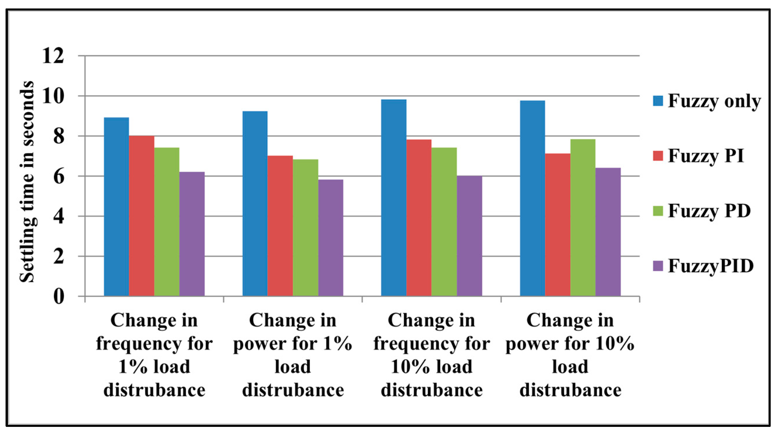
| 0.01 | 8.921 | 8.012 | 7.421 | 6.213 | 9.245 | 7.012 | 6.841 | 5.824 |
| 0.1 | 9.821 | 7.821 | 7.423 | 6.012 | 9.762 | 7.121 | 7.845 | 6.412 |
| Load (p.u) | Change in Frequency (Hz) | Change in Power (p.u) | ||||||
|---|---|---|---|---|---|---|---|---|
| Fuzzy Only | Fuzzy PI | Fuzzy PD | Fuzzy PID | Fuzzy Only | Fuzzy PI | Fuzzy PD | Fuzzy PID | |
| 0.01 | 0.0053 | 0.0048 | 0.0051 | 0.0021 | 0.0024 | 0.0024 | 0.0027 | 0.0009 |
| 0.1 | 0.0281 | 0.0247 | 0.0213 | 0.0191 | 0.0582 | 0.0495 | 0.0467 | 0.0433 |
| Load (p.u) | Change in Frequency (Hz) | Change in Power (p.u) | ||||||
|---|---|---|---|---|---|---|---|---|
| Fuzzy Only | Fuzzy PI | Fuzzy PD | Fuzzy PID | Fuzzy Only | Fuzzy PI | Fuzzy PD | Fuzzy PID | |
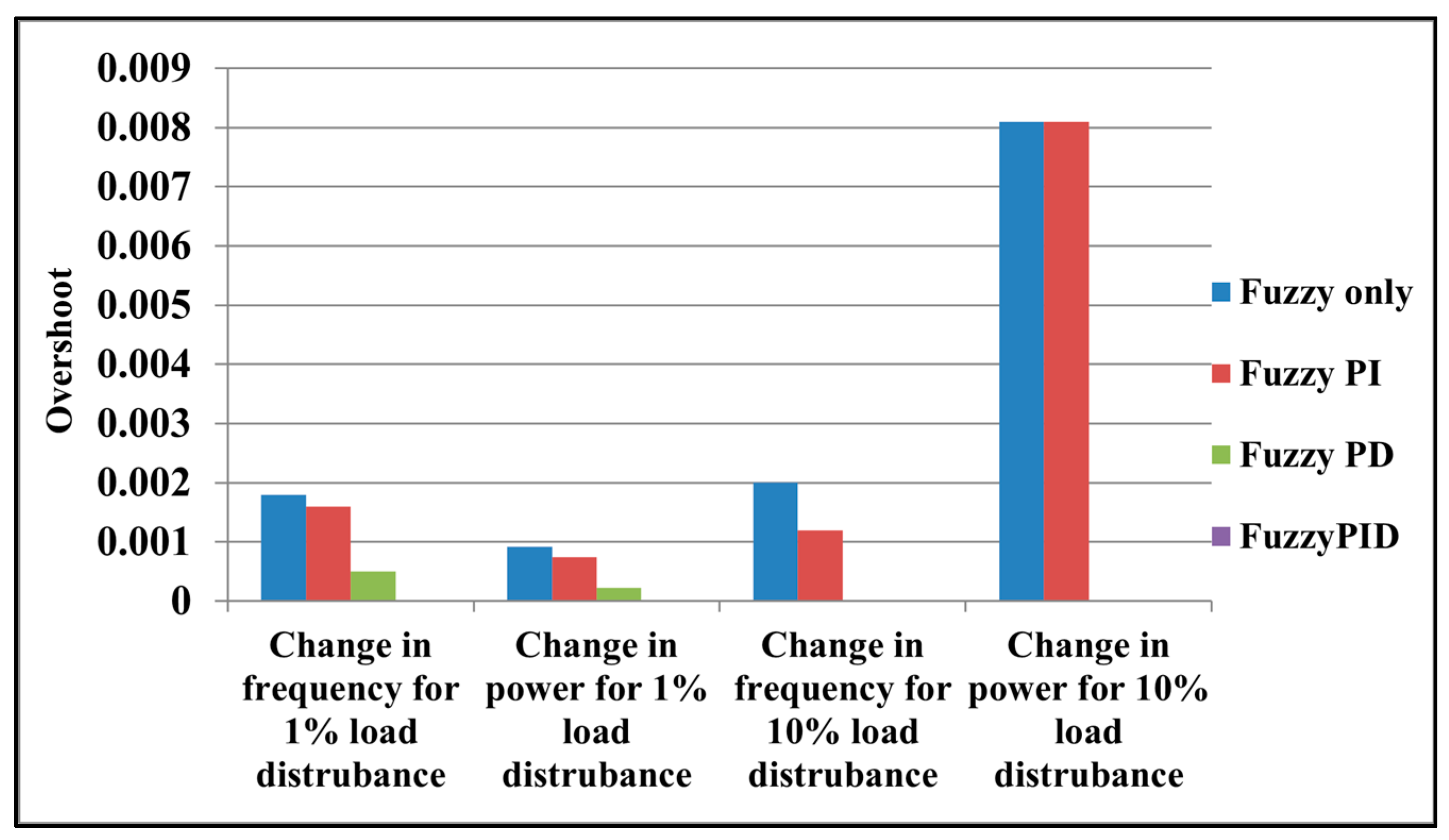
| 0.01 | 0.0018 | 0.0016 | 0.0005 | - | 0.00092 | 0.00075 | 0.00022 | - |
| 0.1 | 0.002 | 0.0012 | - | - | 0.0081 | 0.0081 | - | - |
| Controllers | Parameters | Fuzzy-‘PI’ | Fuzzy-‘PD’ | Fuzzy-‘PID’ |
|---|---|---|---|---|
| Controller-1 | KP1 | 45.2721 | 89.5956 | 20.7350 |
| KI1 | 87.6931 | - | 81.8322 | |
| KD1 | - | 51.5380 | 21.8282 | |
| Controller-2 | KP2 | 12.4553 | 54.4526 | 93.7196 |
| KI2 | 85.8704 | - | 32.4170 | |
| KD2 | - | 60.6446 | 66.8124 |
| Controllers | Parameters | Fuzzy-‘PI’ | Fuzzy-‘PD’ | Fuzzy-‘PID’ |
|---|---|---|---|---|
| Controller-1 | KP1 | 94.1045 | 52.2055 | 71.2286 |
| KI1 | 92.5639 | - | 45.7883 | |
| KD1 | - | 52.5204 | 82.6825 | |
| Controller-2 | KP2 | 52.6068 | 63.7013 | 81.4496 |
| KI2 | 4,300,986 | - | 42.4122 | |
| KD2 | - | 9,109,677 | 93.3730 |
Publisher’s Note: MDPI stays neutral with regard to jurisdictional claims in published maps and institutional affiliations. |
© 2022 by the authors. Licensee MDPI, Basel, Switzerland. This article is an open access article distributed under the terms and conditions of the Creative Commons Attribution (CC BY) license (https://creativecommons.org/licenses/by/4.0/).
Share and Cite
Kumar, N.K.; Gopi, R.S.; Kuppusamy, R.; Nikolovski, S.; Teekaraman, Y.; Vairavasundaram, I.; Venkateswarulu, S. Fuzzy Logic-Based Load Frequency Control in an Island Hybrid Power System Model Using Artificial Bee Colony Optimization. Energies 2022, 15, 2199. https://doi.org/10.3390/en15062199
Kumar NK, Gopi RS, Kuppusamy R, Nikolovski S, Teekaraman Y, Vairavasundaram I, Venkateswarulu S. Fuzzy Logic-Based Load Frequency Control in an Island Hybrid Power System Model Using Artificial Bee Colony Optimization. Energies. 2022; 15(6):2199. https://doi.org/10.3390/en15062199
Chicago/Turabian StyleKumar, Neelamsetti Kirn, Rahul Sanmugam Gopi, Ramya Kuppusamy, Srete Nikolovski, Yuvaraja Teekaraman, Indragandhi Vairavasundaram, and Siripireddy Venkateswarulu. 2022. "Fuzzy Logic-Based Load Frequency Control in an Island Hybrid Power System Model Using Artificial Bee Colony Optimization" Energies 15, no. 6: 2199. https://doi.org/10.3390/en15062199
APA StyleKumar, N. K., Gopi, R. S., Kuppusamy, R., Nikolovski, S., Teekaraman, Y., Vairavasundaram, I., & Venkateswarulu, S. (2022). Fuzzy Logic-Based Load Frequency Control in an Island Hybrid Power System Model Using Artificial Bee Colony Optimization. Energies, 15(6), 2199. https://doi.org/10.3390/en15062199