A Study of the Interface Fluctuation and Energy Saving of Oil–Water Annular Flow

Abstract

Oil–water annular flow is an efficient method of heavy oil transportation for energy-saving. To deeply study the influencing factors of the energy savings of oil–water annular flow, this paper compares the interface fluctuation and energy-saving situation of oil–water annular flow under different pipe structures (such as straight pipe, sudden-contraction pipe, and elbow pipe), flow parameters, and fluid properties. In the straight pipe, the flow parameters can impact the oil–water annular flow pattern and the energy savings, and the interface fluctuation is consistent with the energy savings. The stable oil–water core annular flow has slight interface fluctuation and significant energy savings. At the same time, the influences of pipe structure and fluid properties on energy saving are also analyzed. In the sudden-contraction pipe, the oil–water interface fluctuates, largely due to the sharp changes in flow cross-section, which leads to reduced energy savings. In the elbow, the oil–water interface fluctuates greatly due to the influence of centrifugal force caused by flow direction variation, and also leads to a decline in energy savings. The effects of oil property or annulus liquid property on the interface fluctuates, and the energy savings are analyzed; reducing surface tension is an effective measure to provide an energy-saving effect. These results can provide a reference for the design of heavy-oil-transportation pipelines, the analysis of interface fluctuation, and the energy-saving evaluation of oil–water annular flow.

1. Introduction

Heavy oil–water annular flow is a potential method for heavy oil transportation, whose center is heavy oil, and the annulus is water film. It could reduce the energy consumption of heavy oil transportation in a pipeline [1] and is a low-carbon and cost-effective transportation mode [2]. Even if the oil core sticks to the pipe wall, the pressure drop of heavy oil flow with oil–water annular flow is still much smaller than that of only a single heavy oil flow [3].

Since Isaacs and Speed proposed annular flow technology (oil–water core–annular flow) in 1904 [4], which acted as water-lubricated transportation for heavy oil, it has received attention from many researchers [5]. Charles et al. studied oil–water annular flow, the parts of which were of equal density and different viscosity, and a theoretical model was proposed to obtain the reduction in pressure loss and energy [5]. Hasson et al. conducted an experimental investigation of oil–water annular flow and proposed a water film rupturing condition and oil core break-up condition [6]. Bentwich studied the interface shape and its influencing factors (interfacial tension, capillary forces, and so on), and found that core–annular flow could reduce the pressure by 50% if the viscosity ratio of oil to water was 20 [7]. Ooms et al. hypothesized that the buoyancy of a heavy oil core could be balanced by the dynamic pressure of water annulus and attempted to discuss the stability of oil–water annular flow by using hydrodynamic lubrication theory [8]. Oliemans et al. noted the turbulent behavior in the core–annular flow and proposed empirical correlations for predicting wavelength (which could indicate the pressure gradient) and water holdup [9]. Bai et al. found a new flow pattern (bamboo waves and corkscrew waves) and noted that the pressure loss was minimal under a particular flow rate of water and oil [10]. Miesen et al. used water mixed with sodium silicate solution to prevent the oil core from sticking to the pipe wall [11]. Arney et al. presented the empirical relationship of holdup and water cut and proposed the correlation of friction factor and Reynolds number [12]. Huang et al. studied the influence of oil core eccentricity on the friction factor and found that the friction factor increases under increasing eccentricity [13]. Bai et al. simulated oil–water annular flow to analyze the wave shape, wavelength, pressure gradient, and pressure distribution [14]. Parda and Bannwart proposed a theoretical method to obtain the pressure loss of oil–water annular flow in a vertical pipe and found that the pressure loss of an oil–water annular flow was 45 times smaller than that of a single oil flow [15]. Kao et al. compared the pressure distribution and wavelength of oil–water annular flow under different turbulence models (such as the k-w model, the shear stress transport model) [16]. Ooms and Poesio showed that the lubrication force could counterbalance the buoyance force for snake waves [17]. Bensakhria et al. found that the annular flow could reduce pressure drops by 90% [18]. Rodriguez et al. determined the volume fraction of oil by measuring the wave speed and wavelength [19]. Additionally, they further used the analytical model to predict the wavelength, amplitude, and holdup ratio [20]. Jana et al. showed that the range of annular flow was very limited [21]. Ooms et al. continued to apply a hydrodynamic lubrication model to investigate the development of interfacial waves [22]. Olce et al. performed experiments to analyze the instability of oil–water core annular flow inside a pipe and found instability under some parameters [23]. Sharma et al. presented the hydrodynamics of heavy oil–water annular flow inside a return bend and found that the direction had a great influence on the phase volume fraction [24]. Kaushik et al. investigated oil–water annular flow inside a sudden contraction and expansion pipe, and they noticed that a pressure drop increased suddenly at the contraction while decreasing steeply at the expansion [25]. Ooms et al. compared the pressure distribution of the upper and lower regions of a pipe. The variations of pressure at these parts could lead to wave variation [26]. Jiang et al. analyzed the pressure distributions of oil–water annular flow in a return bend and optimized the operation and geometric parameters [27]. Abubakar et al. investigated the flow patterns of medium-viscosity oil and water flow in a horizontal straight pipe and they revealed that the pressure gradients increased with both mean speeds and inlet oil phase fractions [28]. Loh and Premanadhan conducted an experimental study and found the occurring condition of the flow-transitions regime [29]. Shi et al. compared the accuracy of some pressure-drop models of annular flow, and the flow pattern influenced the pressure drop [30]. Sarmadi et al. used a visco-plastic fluid to eliminate the instabilities of the oil core and explored the impacts of input flow ratios and interfacial shape on the pressure loss [31]. Garmroodi et al. simulated the waxy crude oil–water annular flow in inclined pipes and indicated the regimes of pressure loss varied with the dip angle of the pipe [32].

The above research can help us study the flow patterns of oil and water core–annular flow and the relationship of pressure drops and flows and geometric parameters. A critical component of core–annular flow is energy savings. Some research has involved the energy analysis of annular flow. Brauner analyzed the energy factor of core–annular flow, which is a function of the viscosity ratio of oil and water. They found that the energy factor increases with the decrease in the density difference between the two fluids [33]. Rovinsky et al. found that the energy factor, velocity distribution, and pressure-drop-reduction factor were related to the viscosity ratio of oil and water. The energy factor increases as the viscosity ratio increases and is influenced by the flow rate ratio [34]. Sharma et al. hypothesized that oil–water core–annular flow would be stable to its minimum total energy. They used the energy-minimization approach to investigate the pressure drop and flow pattern [35]. Al-Wahaibi et al. studied the energy of oil–water flow and found the polymer could reduce the pumping energy by about 57.3% [36]. Coelho et al. reported that the energy savings of core–annular flow could be half of single heavy oil transportation [37]. Therefore, investigating the energy-saving situation of oil–water annular flow can provide supporting data for the design of parameters for heavy oil transportation, and it is worth continuing.

In the present work, the interface fluctuation and energy-saving situation of oil and water annular flow in pipes with different structures (such as a horizontal straight pipe, sudden-contraction pipe, and elbow pipe) are examined by using numerical simulation. The influence factor of energy saving will be investigated, and these results will provide a basis for optimizing the operation and geometric parameters for the pipelines design of heavy oil transportation.

2. The Governing Equations

The data in this work come from numerical simulation. To track the two-phase interface, Albadawi et al. compared LS (Level Set), VOF (Volume of Fluid), and CLSVOF (coupled LS with VOF), and found that CLSVOF combines the advantages of VOF (mass conservation) and LS (sharp interface) [38], so the CLSVOF approach is adopted for tracking the oil–water interface, which involves the N-S (Navier–Stokes) equations and LS and VOF equations.

2.1. N-S Equations

The N-S equations continuity equation, the momentum equation of two fluids, can be described as [1,26,27].

$$\nabla \cdot \overrightarrow{u}=0$$

(1)

$$\frac{\partial \left(\rho \overrightarrow{u}\right)}{\partial t}+\nabla \cdot \left(\rho \overrightarrow{u}\overrightarrow{u}\right)=-\nabla p+\nabla \cdot \mu \left(\nabla \overrightarrow{u}+\nabla {\overrightarrow{u}}^T\right)+\rho \overrightarrow{g}+{\overrightarrow{F}}_{\sigma }$$

(2)

where $\rho$ is the fluid density, $\mu$ is the fluid viscosity, $u$ is the velocity, $g$ is the acceleration of gravity, $p$ is the pressure, and $F_{\sigma }$ is the interfacial tension force.

Because the Reynolds number of water is greater than the critical Reynolds number, the turbulence model needs to be used, and the standard $k-\epsilon$ model is used, which are written as follows.

$$\frac{\partial \left(\rho k\right)}{\partial t}+\mathsf{\Delta }\left(\rho kU\right)=\mathsf{\Delta }\left(\frac{{\mu }_t}{{\sigma }_k}\mathsf{\Delta }k\right)+2{\mu }_t{E}_{ij}{E}_{ij}-\rho \epsilon$$

(3)

$$\frac{\partial \left(\rho \epsilon \right)}{\partial t}+\mathsf{\Delta }\left(\rho \epsilon U\right)=\mathsf{\Delta }\left(\frac{{\mu }_t}{{\sigma }_{\epsilon }}\mathsf{\Delta }\epsilon \right)+C_{1\epsilon }\frac{\epsilon }{k}2{\mu }_t{E}_{ij}{E}_{ij}-C_{2\epsilon }\rho \frac{{\epsilon }^2}{k}$$

(4)

$${\mu }_t=C_{\mu }\rho \frac{k^2}{\epsilon }$$

(5)

where $k$ is the turbulent kinetic energy,$\epsilon$ is the dissipation rate, ${\mu }_t$ is the eddy viscosity, and $E_{ij}$ is written as follows.

$$E_{ij}=\frac{1}{2}\left(\frac{\partial U_i}{\partial X_j}+\frac{\partial U_j}{\partial X_i}\right)$$

(6)

The constants are taken as $C_{\mu }=0.09$, ${\sigma }_k=1$, ${\sigma }_{\epsilon }=1.3$, $C_{1\epsilon }=1.44$, $C_{2\epsilon }=1.92$.

2.2. LS Approach

In the LS approach, the LS function ($\varphi$) and Heaviside function (H) are set, which are impacted by the VOF field ($\alpha$), and their relationship is as follows [39]:

$${\varphi }_0=\left(2\alpha -1\right)\mathsf{\Gamma }$$

(7)

$$\frac{\partial \varphi }{\partial \tau }=\mathrm{sign}\left({\varphi }_0\right)\left(1-\left|\nabla \varphi \right|\right)$$

(8)

$$\varphi \left(x,0\right)={\varphi }_0\left(x\right)$$

(9)

where $\mathsf{\Gamma }$ is a dimensionless number, and $\mathsf{\Gamma }=0.75\mathsf{\Delta }x$, $\mathsf{\Delta }x$ is the cell spacing.

2.3. VOF Approach

In the VOF approach, the volume fraction $\alpha$ of oil and water complies with the following conservation equation [1,26,27]:

$$\frac{\partial \alpha }{\partial t}+\overrightarrow{u}\cdot \nabla \alpha =0$$

(10)

The phase volume fraction $\alpha$ is written as

$$\alpha =\{\begin{array}{c} 0\begin{array}{cc}& \mathrm{water}\end{array}\\ 1\begin{array}{cc}& \mathrm{oil}\end{array}\\ 0<\alpha <1\begin{array}{cc}& \mathrm{interface}\end{array}\end{array}$$

(11)

For Equation (2), density $\rho$, and viscosity $\mu$ are written by using ${\alpha }_o$ and ${\alpha }_w$, which are described as

$$\rho ={\alpha }_o{\rho }_o+{\alpha }_w{\rho }_w$$

(12)

$$\mu ={\alpha }_o{\mu }_o+{\alpha }_w{\mu }_w$$

(13)

${\rho }_w$ is the water density, ${\rho }_o$ is oil density, ${\alpha }_o=\alpha$ is the oil volume fraction, while ${\alpha }_w=\left(1-\alpha \right)$ is the water volume fraction; ${\mu }_w$ and ${\mu }_o$ are the water and oil viscosity, respectively.

In Equation (2), for the overall flow, Equations (8) and (9) are used for density and viscosity. For each fluid flow, Equation (2) needs to be modified to the VOF (${\alpha }_o$ or ${\alpha }_w$) of the fluid. For example, for the oil phase, Equation (2) is modified as follows.

$$\nabla \cdot {\alpha }_o\overrightarrow{u_o}=0$$

(14)

$$\frac{\partial \left({\alpha }_o{\rho }_o\overrightarrow{u_o}\right)}{\partial t}+\nabla \cdot \left({\alpha }_o{\rho }_o\overrightarrow{u_o}\overrightarrow{u_o}\right)=-\nabla p+\nabla \cdot \mu \left(\nabla \overrightarrow{u_o}+\nabla {\overrightarrow{u_o}}^T\right)+{\alpha }_o{\rho }_o\overrightarrow{g}+{\overrightarrow{F}}_{\sigma }$$

(15)

In Equation (2), the external force is the surface tension force ${\overrightarrow{F}}_{\sigma }$, and complies with the CSF (continuum surface force) model. The CSF model is described by

$$F_{\sigma }={\sigma }_{ow}\frac{{\alpha }_o{\rho }_o\kappa \nabla {\alpha }_w+{\alpha }_w{\rho }_w\kappa \nabla {\alpha }_o}{0.5\left({\rho }_o+{\rho }_w\right)}$$

(16)

$$\kappa =\nabla \cdot \left(\frac{n}{\left|n\right|}\right)$$

(17)

$$n=\nabla {\alpha }_o$$

(18)

where $F_{\sigma }$ is the surface tension force (external force in Equation (2)), ${\sigma }_{ow}$ is the surface tension coefficient, $n$ is the normal surface for wall adhesion, $n=n_{wall}cos{\theta }_{wall}+t_{wall}sin{\theta }_{wall}$, ${\theta }_{wall}$ is the contact angle, $n_{wall}$ and $t_{wall}$ are the unit normal vector and tangent vector to the wall, respectively, and $\kappa$ is the curvature.

In some cases, the heavy oil is considered as non-Newtonian fluid, and its viscosity is modeled according to the power law, which is described as follows:

$$\mu =K{\left(\dot{\gamma }\right)}^{n-1}$$

(19)

where K is a consistency index; n is a flow behavior index, both chosen empirically; and $\dot{\gamma }$ is the shear rate.

2.4. Coupled LS and VOF (CLSVOF)

In the CLSVOF approach, the LS approach and VOF approach are coupled, and the CSF model varies with the LS approach, which can be expressed as

$$F_{\sigma ,\varphi }={\sigma }_{ow}{k}_{\varphi }{\delta }_{\varphi }\nabla \varphi$$

(20)

in which the delta function ${\delta }_{\varphi }$ is written as

$${\delta }_{\varphi }=\{\begin{array}{c}\frac{1}{2e}(1+cos(\frac{\pi \varphi }{e}))\begin{array}{cc}& \left|\varphi \right|<e\end{array}\\ 0\begin{array}{cc}& \mathrm{elsewhere}\end{array}\end{array}$$

(21)

where e is the interface thickness, $e=1.5\mathsf{\Delta }x$.

The physical properties in Equation (2) can be computed by using the Heaviside function:

$$H\left(\varphi \right)=\{\begin{array}{c}0\begin{array}{cc}& \varphi <-e\end{array}\\ \frac{1}{2}[1+\frac{\varphi }{e}+\frac{1}{\pi }sin(\frac{\pi \varphi }{e})]\begin{array}{cc}& \left|\varphi \right|\ge e\end{array}\\ 1\begin{array}{cc}& \varphi >e\end{array}\end{array}$$

(22)

Some dimensionless numbers used in this work are described as follows [1,12,27,36].

(1) Water cut, ${\epsilon }_w$

$${\epsilon }_w=Q_w/Q_T$$

(23)

where $Q_w$ is the water rate of flow, $Q_T$ is the rate of total volumetric flow, and $Q_T=Q_w+Q_o$.

(2) The area-weighted average of oil volume fraction, ${\alpha }_o$

$${\alpha }_o=\frac{1}{A}{{\displaystyle \sum }}_{i=0}^n{\alpha }_{oi}{A}_i$$

(24)

where $A_i$ is the area occupied by oil, and A is the area of the cross-section of the pipe.

${\alpha }_o$ could be obtained using the empirical formula proposed by Arney et al. [13], which is expressed as

$${\alpha }_o=1-{\epsilon }_w\left[1+0.35\left(1-{\epsilon }_w\right)\right]$$

(25)

(3) Head loss, h_L

The head loss in the pipe should be in the form of the energy-saving index, and it can be defined as

$$h_L=\frac{\Delta P}{{\rho }_{m}g}$$

(26)

where ΔP is the pressure drop, and ${\rho }_m={\epsilon }_w{\rho }_w+\left(1-{\epsilon }_w\right){\rho }_o$ is the mixture density.

3. Numerical simulation

3.1. Geometry

In these simulations, four pipe structures are considered as the flow domain, which are the straight pipe, the sudden-contraction pipe, the elbow pipe, and the return pipe, as shown in Figure 1.

3.2. Mesh Generation of the Flow Domain

The above geometries of the flow domain are meshed by ANSYS Workbench Mesh. The results of the cell and node are listed in

Table 1. The cells and nodes of flow domains.

Flow Domain	Number of Cells	Number of Nodes
Horizontal pipe	225,240	231,495
Sudden-contraction pipe	1,987,200	2,020,681
Elbow pipe	1,117,200	1,137,236
Return pipe	177,185	187,327

. Because the computational accuracy can be influenced by the geometry’s discretization, in our earlier studies [1,40], the cell convergence was validated, and we concluded that this cell number was sufficient.

3.3. Solution Strategy

The package OpenFOAM and the package Fluent are used for these simulations. The CLSVOF model is employed to describe a clear interface between oil and water. In the OpenFOAM package, the pressure–velocity coupling is performed by the PISO scheme. A second-order upwind scheme is used for momentum, turbulent kinetic energy, and the dissipation rate [1]. In the Fluent package, the pressure–velocity coupling is implemented by the SIMPLE (Semi-Implicit Method for Pressure Linked Equation) algorithm. The turbulence model adopts standard k-ε [39]. The convergence criteria are chosen according to the residual value of the calculated variables (such as mass, velocity components, and volume fraction). For computational cases in both packages, the convergence criterion is set to be 10⁻³ for all variables.

3.4. The Boundary Conditions and the Parameters

For the horizontal straight pipe (using OpenFOAM solver, because it is easier to set the periodic boundary conditions), a periodic boundary condition was employed in the axial direction. The pressure drop was set at two ends and remained the same during the calculation. The pipe wall was set to the no-slip, no penetration boundary condition [1]. The computational domain was initially filled with the ideal oil–water annular flow, in which the initial oil core diameter d is given by the water volume fraction. The viscosities of the two fluids were μ_o = 0.697 Pa·s and μ_w = 0.00067 Pa·s, respectively; the densities were ρ_o = 901.49 kg/m³ and ρ_w = 993.15 kg/m³, respectively; and the interfacial tension between the two fluids was σ = 1.6 ×10⁻² N/m.

For other pipes (using Fluent solver, because it is more efficient), the oil velocity was set at the core region, $v_x=v_{oil}$, and the water velocity was set at the annulus region, $v_x=v_{water}$; $v_{water}, v_{oil},$ adjusted according to the working conditions. The pipe wall was set as a stationary, no-slip ($v_x=0$), no penetration ($v_r=0$) boundary. In addition, a contact angle (${\theta }_{wall}={27}^{°}$) between water and pipe wall material was set at the wall. The pressure outlet boundary was considered on the outlet [26,27,28,29]. The initial fluids were considered with lube oil (ρ_o = 960 kg/m³ and μ_o = 0.22 Pa·s) at the center, and water (ρ_w = 998.2 kg/m³ and μ_w = 0.001003 Pa·s) at the annulus.

4. Results and Discussions

To validate the numerical results, seven cases are calculated, where ε_w is varied from 0.072 to 0.1293. The simulated results are compared with the empirical data, as presented in Figure 2. It is evident that the numerical predictions are consistent with the empirical results [12].

Furthermore, the head losses between the single oil flow and oil–water flow are compared, under the conditions of the water cut being 0.19 and average velocity being 0.8–1.6 m/s, and the comparison results are depicted in Figure 3. According to Figure 3, the energy savings of oil–water annular flow is very significant; this is because the water film wrapped the oil flow in the center region and avoided the direct friction between the oil core and pipe wall, which led to a smaller pressure drop. Figure 4 shows some oil–water annular flow behaviors in the horizontal straight pipe. The oil–water interfaces with different water cuts (${\epsilon }_w$) indicate that with the increase in the water cut, the interface wave amplitude increases, the oil core floats above the pipeline, and the upper interface wave amplitude is less than the lower interface wave amplitude.

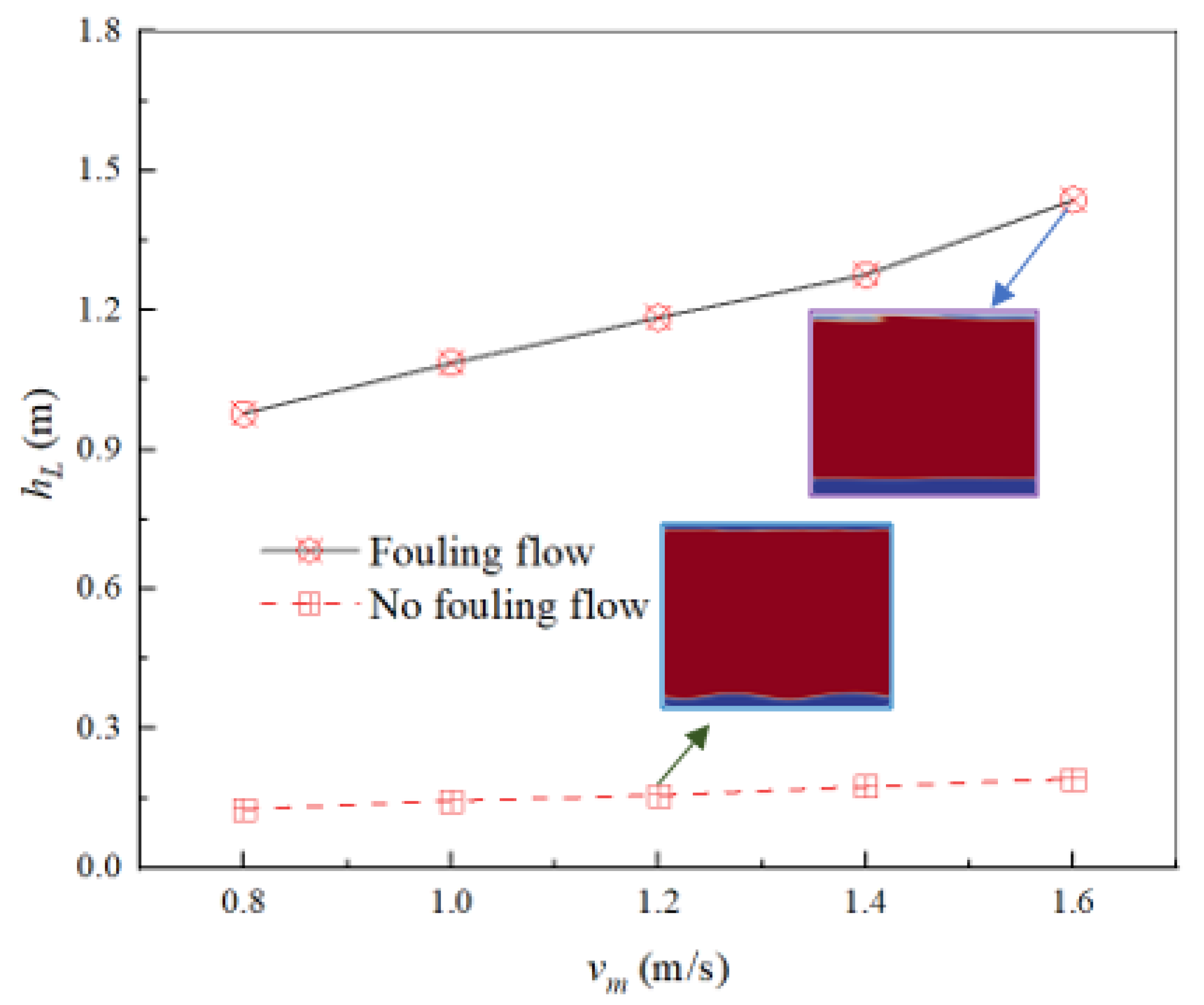
4.1. The Effect of Flow Parameters

The parameters of oil and water core–annular flow impact transportation energy consumption. As can be seen from Figure 3, the head loss increases when the average velocity increases. The reason for this is that the flow resistance increases with the increase in the flow velocity, resulting in the increase in the pressure drop.

The influence of the water cut on head loss is further investigated, which is shown in Figure 5. With the increase in the water cut, the head loss increases. The reason for this is that the smaller the water cut, the thinner the water film, and the smaller the resistance, the smaller the pressure drop. This tendency shows no difference from the experimental data of Al Wahaibi et al. [36].

When the oil–water annular flow loses stability and sticks to the wall, the head loss will increase sharply and increase the energy consumption (see Figure 6) because the fouling flow leads to a rapidly increased pressure drop. However, this is still less than the single oil flow; Shi et al. stated that the pressure drop, even under the condition of core–annular flow with oil fouling, is still lower than the pressure drop of the single oil flow [3].

The core–annular flow is stable under certain flow conditions (the water cut is more than 0.97 in this work). Only by stabilizing the annular flow can energy savings be achieved, and the instability of core–annular flow will lead to a marked increase in transportation energy consumption. Figure 7 depicts the top oil–water interface wave of oil–water annular flow under stable and unstable conditions. After the interface wave experiences instability, the interface wave crest will adhere to the pipe wall, the oil core will hinder the flow, and an increase in the pressure drop will follow. Therefore, keeping an appropriate water cut and flow rate (or average velocity) has an essential impact on the stability of core–annular flow and energy savings.

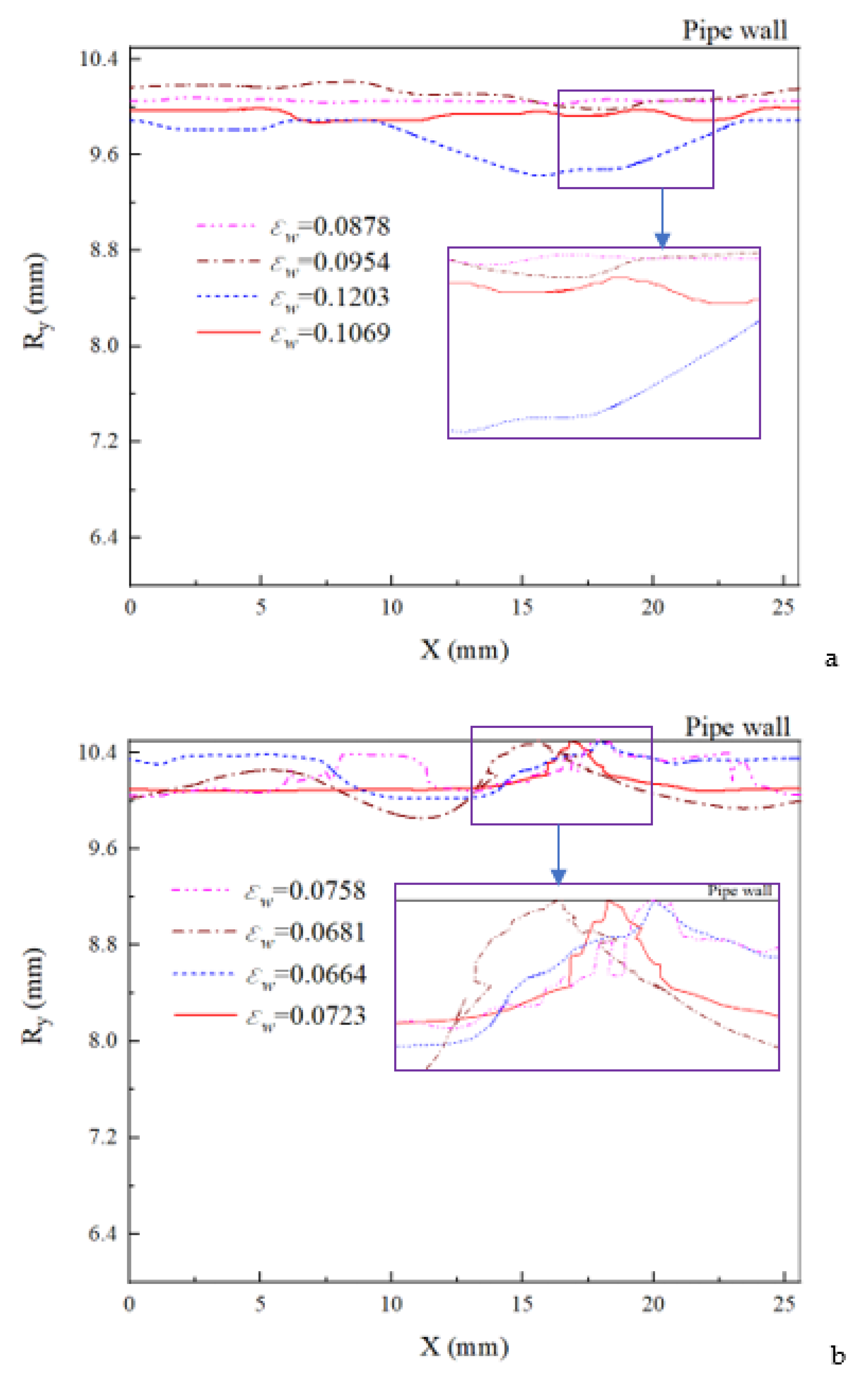
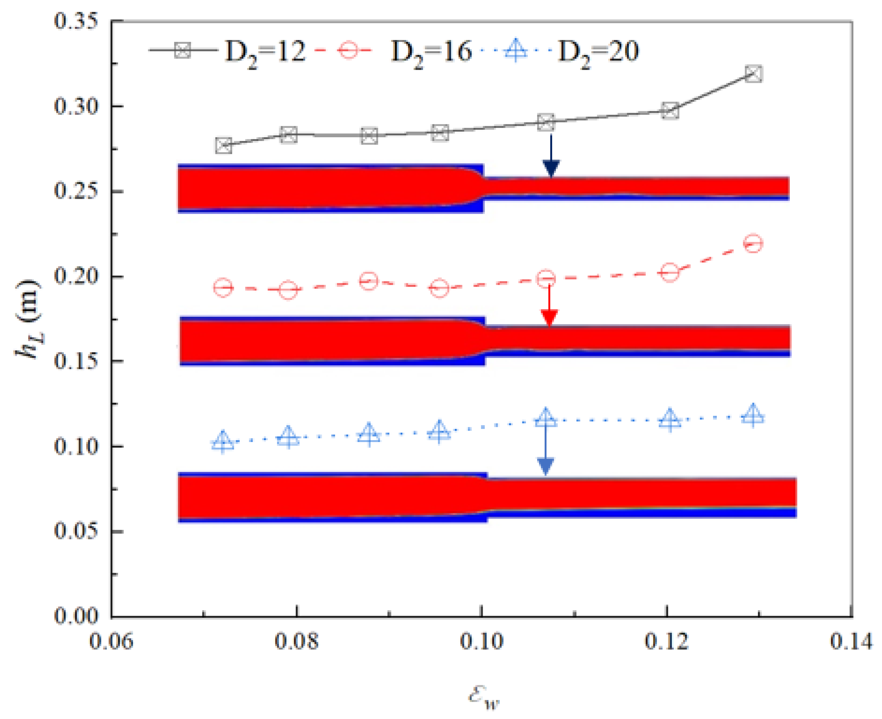
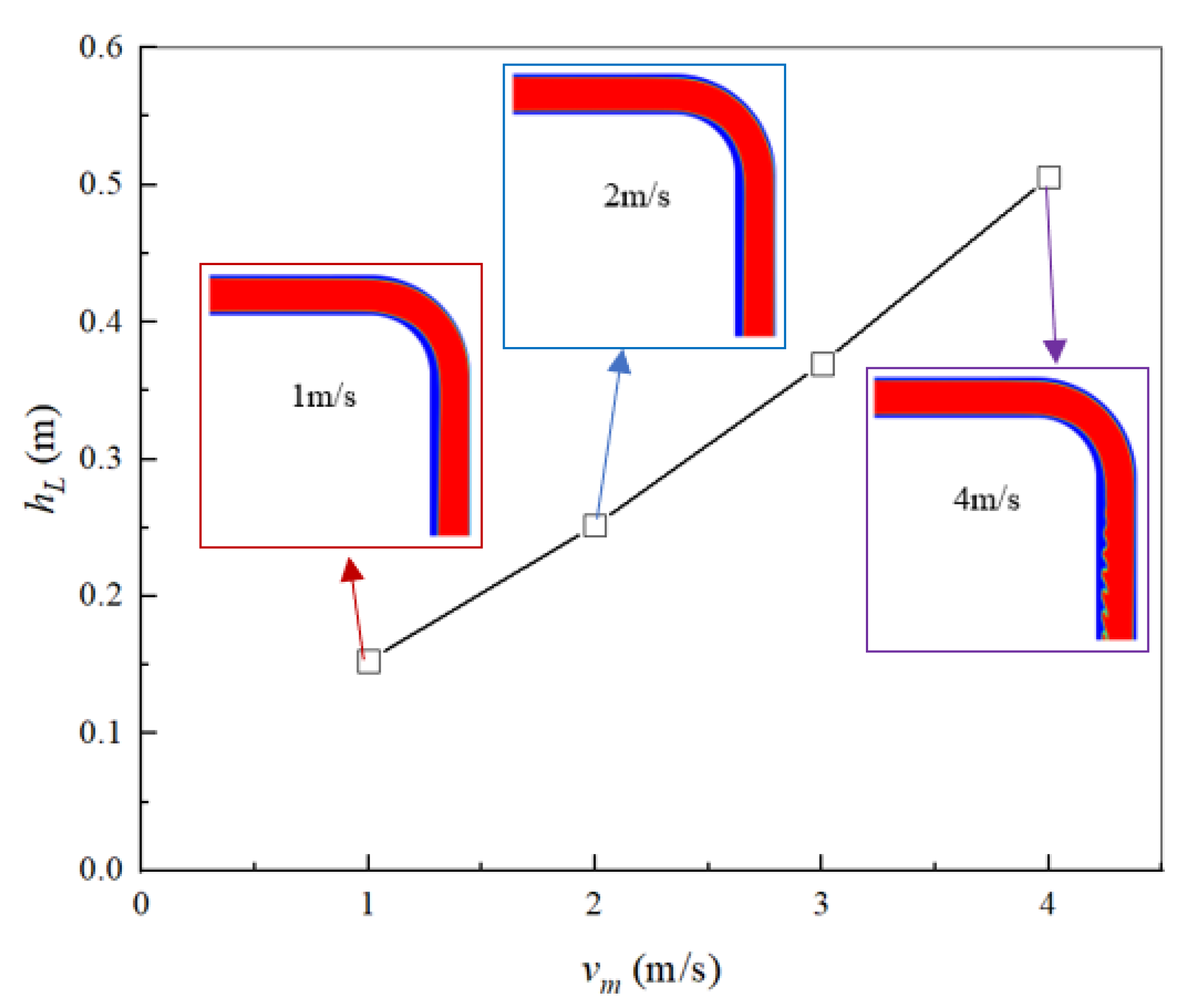
4.2. The Effect of Structures

Figure 5 depicts the head loss difference between the horizontal straight pipe and sudden-contraction pipe. In the present work, four different structures are considered (see Figure 1), and the structural parameters of these pipelines are also changed.

For the sudden-contraction pipe, the sharp change of the flow section leads to a large local head loss. While the oil–water core–annulus flows through in the sudden-contraction pipe, via the action of secondary flow, a turbulent vortex is formed in the water annulus at the diameter-reduction location, which destroys the stability of the core–annular flow, increases the pressure drop, and leads to an increase in the head loss. According to Figure 8, the oil–water annular flow is shown under different water superficial velocities ($v_w=0.1472-0.8832\mathrm{m}\mathrm{/}\mathrm{s}$). When the water velocity enlarges, the downstream oil–water annular flow gradually reaches instability. As water velocity is larger than 0.736 m/s, the annular flow downstream of the sudden-contraction pipe is unstable. Figure 5 also shows that the head loss increases with the increase in the water cut, which is due to the oil–water annulus leading to instability downstream.

When the contraction area ratio of the sudden-contraction pipe is changed, the flow pattern of core–annular flow is varied, and the local head loss is also changed, as shown in Figure 9.

The elbow pipe, due to the change of flow direction, also produces a local head loss, which increases the transportation energy consumption. Figure 10 represents the pattern of oil–water annular flow and the head loss in the 90° elbow pipe. When the flow velocity increases, the head loss increases. When the flow velocity exceeds 4 m/s, the oil–water interface loses its stability.

Figure 11 compares the oil–water annular water head loss of elbows with different curvatures. When the curvature is smaller, the centrifugal force is greater, the secondary flow and vortex intensity are greater, and the interface fluctuation is more intense, resulting in a greater local head loss. As the curvature increases, the pressure drop and the local head loss decreases.

For the return bend, the change of flow direction is greater than the elbow, resulting in greater local head loss, as shown in Figure 12. When the flow velocity of water is less than or much greater than the flow velocity of oil under certain conditions of initial water holdup, the oil–water interface will be unstable, resulting in an increased head loss.

From the above analysis, the pipe structures impact the interface wave and energy saving of oil–water annular flow. Reducing the variation of pipe structure (variation of the flow’s cross-section and direction) is very helpful to keep the stability of the oil–water annular flow and maintain a good energy-saving effect.

4.3. The Effect of Fluids’ Properties

When changing the properties of oil and water, the state of two-phase flow and head loss will be changed. In the sudden-contraction pipe, four CTAC (cetyltrimethylammonium chloride) solutions are selected to replace water (the water annulus is replaced by the CTAC solution annulus). The surfactant can significantly inhibit the interface wave development and reduce head loss, as shown in Figure 13. Figure 13 compares the results between the water annulus in the sudden-contraction pipe and the other four solutions’ annuli. The higher the concentration of the surfactant solution in the solution annulus, the lower the head loss, mainly because the surfactant reduces the surface tension.

Figure 14 shows the conditions of the top (Figure 14a) and bottom (Figure 14b) of oil–water interfaces of the sudden-contraction pipe downstream with different surfactant solution annuli (CTAC0 is pure water). The amplitude of the interface fluctuation decreases with the increase in the surfactant concentration.

When the property of the oil core is varied, the head loss is also varied. Five viscous oils are considered, whose densities are the same, and viscosities are 0.697, 0.787, 0.9182, 1.335, and 1.9931 Pa·s, respectively. When the oil core viscosity increases within a specific range, the head loss will gradually decrease, as depicted in Figure 15. After the oil core viscosity increases, the oil core rigidity increases, the oil–water interface does not easily destabilize, and the transportation pressure drop is small; this trend is in agreement with the results of our previous work [1] on the fouling limit of oil and water annular flow.

In the oil–water annular downflow in a return bend with v_so = 0.15 m/s and v_sw = 0.3 m/s, seven non-Newtonian oils (see

Table 2. Physical properties of non-Newtonian oil [41] and h_L.

Oil Name	Density (kg/m3)	Fluid Consistency Coefficient	Flow Behavior Index	Surface Tension (N/m)	hL under v = 0.8 m/s	hL under v = 1 m/s
CMC1	999.9	0.089	0.789	0.0714	0.130	0.152
CMC2	1000.0	0.469	0.658	0.0718	0.231	0.256
CMC3	1000.4	0.972	0.615	0.0727	0.264	0.275
CMC4	1000.8	0.00218	0.948	0.0735	0.129	0.143
CMC5	1001.2	0.00419	0.910	0.0745	0.133	0.148
CMC6	1001.3	0.00588	0.871	0.075	0.141	0.151
CMC7	1001.5	0.00692	0.850	0.0755	0.146	0.161

) are simulated, and the impact of oil properties on head loss are presented in Table 2. With the increase in density, viscosity, and surface tension, the head loss increases, in which viscosity and surface tension are the main influencing factors. As the interfacial tension increases, the interface wave instability of oil and water increases. The oil core will break through the water film in the case of large interface fluctuations, causing wall adhesion and a pressure drop, which is consistent with our previous analysis’s results [41].

The above results reveal the consequences of fluids’ properties on the energy savings of oil and water flow. Reducing the surface tension between the two fluids is an important means to maintain the stability of annular flow and reduce energy consumption.

5. Conclusions

Oil–water annular flow is an energy-saving approach for heavy oil transportation, but its energy saving is impacted by flow parameters, pipe structure, fluid properties, and so on. In this work, the influencing factors and trends of the energy saving of oil and water flow are discussed, and the following conclusions are obtained.

The flow parameter is an essential factor in keeping the stability of oil–water annular flow. Appropriate flow parameters (oil–water flow rate, water cut, etc.) should be used to keep interface fluctuation slight and maintain the stability of annular flow, and a better energy saving can be obtained.

The change of pipe structure impacts the energy-saving effect of core–annular flow. In engineering practice, the change of pipe section and flow direction should be minimized so as to reduce the chance of the core–annular losing stability and to keep good energy savings.

The variation of the two-phase fluid properties of core–annular flow influences the flow state and energy-saving effect of annular flow, among which the viscosity and surface tension have significant influence. Reducing the surface tension between the two phases can help to achieve better energy savings.

Oil–water interface fluctuation is bad for energy savings; the control methods of oil–water interface fluctuation are different in pipelines with different structures. Interface fluctuation is mainly inhibited by controlling flow parameters and adding a surfactant.

References

1. Jiang, F.; Li, H.Y.; Mathieu, P.; Gijs, O.; Ruud, H. Simulation of the hydrodynamics in the onset of fouling for oil-water core-annular flow in a horizontal pipe. J. Pet. Sci. Eng. 2021, 207, 109084. [Google Scholar] [CrossRef]
2. Praveen, K.; Jashanpreet, S. Computational study on effect of Mahua natural surfactant on the flow properties of heavy crude oil in a 90° bend. Mater. Today: Proc. 2021, 43, 682–688. [Google Scholar]
3. Shi, J.; Lao, L.; Yeung, H. Water-lubricated transport of high-viscosity oil in horizontal pipes: The water holdup and pressure gradient. Int. J. Multiph. Flow 2017, 96, 70–85. [Google Scholar] [CrossRef] [Green Version]
4. Joseph, D.D.; Bai, R.; Chen, K.P.; Renardy, Y.Y. Core-annular flows. Annu. Rev. Fluid Mech. 1997, 29, 65–90. [Google Scholar] [CrossRef] [Green Version]
5. Charles, M.E.; Govier, G.W.; Hodgson, G.W. The horizontal pipeline flow of equal density oil-water mixtures. Can. J. Chem. Eng. 1961, 39, 27–36. [Google Scholar] [CrossRef]
6. Hasson, D.; Mann, U.; Nir, A. Annular flow of two immiscible liquids. I. Mechanisms. Can. J. Chem. Eng. 1970, 48, 514–520. [Google Scholar] [CrossRef]
7. Bentwich, M. Two-phase axial laminar flow in a pipe with naturally curved surface. Chem. Eng. Sci. 1971, 31, 71–76. [Google Scholar] [CrossRef]
8. Ooms, G.; Segal, A.; Vanderwees, A.J.; Meerhoff, R.; Oliemans, R.V.A. A theoretical model for core-annular flow of a very viscous oil core and a water annulus through a horizontal pipe. Int. J. Multiph. Flow 1984, 10, 41–60. [Google Scholar] [CrossRef]
9. Oliemans, R.V.A.; Ooms, G.; Wu, H.L.; Duijvestijn, A. Core annular oil/water flow: The turbulent-lubricating–film model and measurements in a 5 cm pipe loop. Int. J. Multiph. Flow 1987, 13, 23–31. [Google Scholar] [CrossRef]
10. Bai, R.; Chen, K.; Joseph, D.D. Lubricated pipelining: Stability of core-annular flow: Part 5, Experiments and comparison with theory. J. Fluid Mech. 1992, 240, 97–132. [Google Scholar] [CrossRef]
11. Miesen, R.; Beijnon, G.; Duijvestijn, P.E.M.; Oliemans, R.V.A.; Verheggen, T. Interfacial waves in core annular flow. J. Fluid Mech. 1993, 238, 97–117. [Google Scholar] [CrossRef]
12. Arney, M.S.; Bai, R.; Guevara, E.; Joseph, D.D.; Liu, K. Friction factor and hold up studies for lubricated pipelining-1. Experiments and correlations. Int. J. Multiph. Flow 1993, 19, 1061–1067. [Google Scholar] [CrossRef]
13. Huang, A.; Christodoulou, C.; Joseph, D.D. Friction factor and hold up studies for lubricated pipelining part. 2: Laminar and k–e models of eccentric core flow. Int. J. Multiph. Flow 1994, 20, 481–491. [Google Scholar] [CrossRef]
14. Bai, R.; Kelkar, K.; Joseph, D.D. Direct simulation of interfacial waves in a high viscosity ratio and axisymmetric core annular flow. J. Fluid Mech. 1996, 327, 1–34. [Google Scholar] [CrossRef] [Green Version]
15. Parda, V.J.W.; Bannwart, A.C. Modeling of vertical core-annular flows and application to heavy oil production. J. Energy Resour. Technol. 2001, 123, 194–199. [Google Scholar] [CrossRef]
16. Kao, T.; Choi, H.G.; Bai, R.; Joseph, D.D. Finite element method simulation of turbulent wavy core-annular flows using a k–w turbulence model method. Int. J. Multiph. Flow 2002, 28, 1205–1222. [Google Scholar] [CrossRef]
17. Ooms, G.; Poesio, P. Stationary core-annular flow through a horizontal pipe. Phys. Rev. E 2003, 68, 066301. [Google Scholar] [CrossRef] [Green Version]
18. Bensakhria, A.; Peysson, Y.; Antonini, G. Experimental study of the pipeline lubrication of heavy oil transport. Oil Gas Sci. Technol. Rev. D IFP Energ. Nouv. 2004, 59, 523–533. [Google Scholar] [CrossRef]
19. Rodriguez, O.M.H.; Bannwart, A.C. Experimental study on interfacial waves in a vertical core flow. J. Pet. Sci. Eng. 2006, 54, 140–148. [Google Scholar] [CrossRef]
20. Rodriguez, O.M.H.; Bannwart, A.C. Analytical model for interfacial waves in vertical core flow. J. Pet. Sci. Eng. 2006, 54, 173–182. [Google Scholar] [CrossRef]
21. Jana, A.K.; Das, G.; Das, P.K. Flow regime identification of two-phase liquid–liquid upflow through vertical pipe. Chem. Eng. Sci. 2006, 61, 1500–1515. [Google Scholar] [CrossRef]
22. Ooms, G.; Vuik, C.; Poesio, P. Core-annular flow through a horizontal pipe: Hydrodynamic counterbalancing of buoyancy force on core. Phys. Fluids 2007, 19, 092103. [Google Scholar] [CrossRef]
23. Selvam, B.; Talon, L.; Lesshaft, L.; Meiburg, E. Convective/absolute instability in miscible core. J. Fluid Mech. 2009, 618, 323–348. [Google Scholar] [CrossRef] [Green Version]
24. Sharma, M.; Ravi, P.; Ghosh, S.; Das, G.; Das, P.K. Hydrodynamics of lube oil–water flow through 180° return bends. Chem. Eng. Sci. 2011, 66, 4468–4476. [Google Scholar] [CrossRef]
25. Kaushik, V.V.R.; Sumana, G.; Gargi, D.; Prasanta, K.D. CFD simulation of core annular flow through sudden contraction and expansion. J. Pet. Sci. Eng. 2012, 86–87, 153–164. [Google Scholar] [CrossRef]
26. Ooms, G.; Pourquié, M.J.B.M.; Beerens, J.C. On the levitation force in horizontal core-annular flow with a large viscosity ratio and small density ratio. Phys. Fluids 2013, 25, 032102. [Google Scholar] [CrossRef]
27. Jiang, F.; Wang, Y.; Ou, J.J.; Xiao, Z.M. Numerical simulation on oil-water annular flow though the π bend. Ind. Eng. Chem. Res. 2014, 53, 8235–8244. [Google Scholar] [CrossRef]
28. Abubakar, A.; Al-Wahaibi, Y.; Al-Wahaibi, T.; Al-Hashmi, A.; Al-Ajmi, A.; Eshrati, M. Effect of low interfacial tension on flow patterns, pressure gradients and holdups of medium-viscosity oil/water flow in horizontal pipe. Exp. Therm. Fluid Sci. 2015, 68, 58–67. [Google Scholar] [CrossRef]
29. Loh, W.L.; Premanadhan, V.K. Experimental investigation of viscous oil-water flows in pipeline. J. Pet. Sci. Eng. 2016, 147, 87–97. [Google Scholar] [CrossRef]
30. Shi, J.; Gourma, M.; Yeung, H. CFD simulation of horizontal oil-water flow with matched density and medium viscosity ratio in different flow regimes. J. Pet. Sci. Eng. 2017, 151, 373–383. [Google Scholar] [CrossRef] [Green Version]
31. Parisa, S.; Ian, A.F. Stable core-annular horizontal flows in inaccessible domains via a triple-layer configuration. Chem. Eng. Sci.: X 2019, 3, 100028. [Google Scholar]
32. Brauner, N. Two-phase liquid liquid annular flow. Int. J. Multiph. Flow 1991, 17, 59–76. [Google Scholar] [CrossRef]
33. Rovinsky, J.; Brauner, N.; Moalem, M.D. Analytical solution for laminar two-phase flow in a fully eccentric core annular configuration. Int. J. Multiph. Flow 1997, 23, 523–543. [Google Scholar] [CrossRef]
34. Garmroodi, M.; Ahmadpour, A. A numerical study on two-phase core-annular flows of waxy crude oil/water in inclined pipes. Chem. Eng. Res. Des. 2020, 159, 362–376. [Google Scholar] [CrossRef]
35. Sharma, A.; Al-Sarkhi, A.; Sarica, C.; Zhang, H.Q. Modeling of oil–water flow using energy minimization concept. Int. J. Multiph. Flow 2011, 37, 326–335. [Google Scholar] [CrossRef]
36. Al-Wahaibi, T.; Abubakar, A.; Al-Hashmi, A.R.; Al-Wahaibi, Y.; Al-Ajmi, A. Energy analysis of oil-water flow with drag-reducing polymer in different pipe inclinations and diameters. J. Pet. Sci. Eng. 2017, 149, 315–321. [Google Scholar] [CrossRef]
37. Coelho, N.M.D.A.; Taqueda, M.E.S.; Souza, N.M.O.; de Paiva, J.L.; Santos, A.R.; Lia, L.R.B.; de Moraes, M.S.; de Moraes, D., Jr. Energy Savings on Heavy Oil Transportation through Core Annular Flow Pattern: An Experimental Approach. Int. J. Multiph. Flow 2020, 122, 103127. [Google Scholar] [CrossRef]
38. Albadawi, A.; Donoghue, D.B.; Robinson, A.J.; Murray, D.B.; Delauré, Y.M.C. On the analysis of bubble growth and detachment at low Capillary and Bond numbers using Volume of Fluid and Level Set methods. Chem. Eng. Sci. 2013, 90, 77–91. [Google Scholar] [CrossRef]
39. Yamamoto, F.; Okano, Y.; Dost, S. Validation of the S-CLSVOF method with the density-scaled balanced continuum surface force model in multiphase systems coupled with thermocapillary flows. Int. J. Numer. Method Fluids 2017, 83, 223–244. [Google Scholar] [CrossRef]
40. Jiang, F.; Wang, K.; Skote, M.; Wong, T.N.; Duan, F. The effects of oil property and inclination angle on oil–water core annular flow through U-Bends. Heat Transf. Eng. 2018, 39, 536–548. [Google Scholar] [CrossRef]
41. Jiang, F.; Wang, K.; Skote, M.; Wong, T.N.; Duan, F. Simulation of non-Newtonian oil-water core annular flow through return bends. Heat Mass Transf. 2018, 54, 37–48. [Google Scholar] [CrossRef]
Figure 1. The geometries of pipe structures. (a) The straight pipe; (b) The sudden-contraction pipe; (c) The elbow pipe; (d) The return pipe.
Energies 15 02123 g001
Figure 2. Comparison of numerical and empirical results.
Energies 15 02123 g002
Figure 3. Comparison of single oil flow and oil–water annular flow.
Energies 15 02123 g003
Figure 4. Oil–water core–annular flow in horizontal pipe ((a) ε w = 0.0877 ; (b) ε w = 0.0954 ; (c) ε w = 0.1203 ; red is oil, blue is water, which means the same later).
Energies 15 02123 g004
Figure 5. The effect of water cut on head loss.
Energies 15 02123 g005
Figure 6. The effect of stability condition on head loss (the input pressure drop is 600–1500 Pa).
Energies 15 02123 g006
Figure 7. The top interfacial wave on the top of pipe. (a) No fouling; (b) fouling.
Energies 15 02123 g007
Figure 8. The oil–water annular flow inside the sudden-contraction pipe. ( v w = 0.1472 0.8832   m / s ,     v o = 0.7056   m / s ).
Energies 15 02123 g008
Figure 9. The effect of area ratio on the head loss.
Energies 15 02123 g009
Figure 10. The head loss and the oil–water core–annular flow in the elbow (90° elbow; the same velocity of oil and water).
Energies 15 02123 g010
Figure 11. The head loss and the oil–water core–annular flow in the elbows with different R/D (90° elbow; the oil and water velocity is 1 m/s).
Energies 15 02123 g011
Figure 12. The head loss and the oil–water core–annular flow in the return bend (vo = 0.6 m/s).
Energies 15 02123 g012
Figure 13. The head loss and surface tension in the sudden-contraction pipe.
Energies 15 02123 g013
Figure 14. The interface at the sudden-contraction pipe downstream. (a) top interface; (b) bottom interface.
Energies 15 02123 g014
Figure 15. The head loss of oil–water annular flow with different oil viscosities.
Energies 15 02123 g015