Studying the Wake of a Tidal Turbine with an IBM-LBM Approach Using Realistic Inflow Conditions

Abstract

The lattice Boltzmann method is used to model a horizontal axis tidal turbine. Because tidal turbines generally operate in highly turbulent flows, a synthetic eddy method is implemented to generate realistic turbulent inflow condition. The approach makes use of the open-source code Palabos. Large eddy simulation is employed. A coupling between an immersed boundary method and a wall model is realized to model the turbine. Calculations are performed at two different turbulence rates. The upstream flow condition is first set up to match with experimental results. Numerical simulations of a tidal turbine with realistic turbulent inflow conditions are then realized with the lattice Boltzmann method. The approach is found to be in good agreement with experimental data. Cases with three different inflow turbulence rates are simulated. An almost linear evolution with the turbulence rate is observed for the axial velocity deficit. An analysis of the propagation of tip-vortices in the close wake is carried out. It is found that turbulence has a great impact on the tip-vortices propagation envelope.

1. Introduction

Worldwide energy consumption keeps increasing and some areas still do not have access to electricity. In order to provide more clean energy, new concepts have been created by academia and industry. Among those concepts are renewable marine energy devices and more precisely tidal turbines. Resulting from gravitational forces, tidal forces create a periodic movement of ocean water level [1]. Induced displacements are not constant and can highly vary from one place to another. In some sites, they create a strong current, like in the Alderney Race where it can go up to 5 ms${}^{-1}$. Using lift generating devices such as airfoils, tidal turbines extract the kinetic power from those currents. Interactions between tidal flows and their environments (sea bottom, coast, wind) may result in the creation of turbulent structures in the flow [2]. Several in site campaigns have already been performed to evaluate the turbulence rate of tidal sites. Thomson et al. [3] measured a turbulence rate between 8.4% and $11.4\%$ in Puget Sound, USA. Turbulence can also vary along the tidal cycle of a specific site. Milne et al. [4] observed that the stream-wise turbulence rate varies between $7\%$ and more than $20\%$ along a tidal cycle at the sound of Islay, Scotland. The project Turbulence In Marine Environment (TIME) [2] lists several problems associated with marine turbulence. It quotes that turbulence may affect the turbines’ integrity, performance and hydrodynamics. To understand turbulence’s influence on tidal turbines, experiments in flume tanks have been carried out. Chen et al. [5] realized an experimental study of the wake, which is critical for the placement of tidal turbines in a farm. Mycek et al. [6] showed that turbulence greatly affects wake recovery and turbine performances. Blackmore et al. [7] showed that high turbulence rates can generate thrust fluctuation up to $20\%$, increasing fatigue failure risk. A good understanding of the turbulence influence on a tidal turbine is thus necessary in order to go from prototype to full industrial exploitation. In addition to flume experiments and in situ measurements, computational fluid dynamics (CFD) has also been used to gather such knowledge.

CFD simulations can be divided into two categories, steady simulations and unsteady simulations. Steady models have already proven their capability of predicting the performance of tidal turbines [8]. However, turbulence is chaotic and steady models may miss some important features of turbulent flows. Unsteady simulations can capture those phenomena. Several unsteady approaches have already been carried out. Elie et al. [9] and Grondeau et al. [10] used actuator large eddy simulation (LES) approaches to model tidal turbines. Their approaches do not model the geometry of the blade but rather represent it with a force. Forces coefficients, medium and far wake are correctly computed. Those kinds of methods cost less computational resources than geometry resolved LES and are well suited for far wake propagation and tidal farm studies. However, a priori knowledge of the blade behaviour is required. Geometry resolved LES simulations of tidal turbines have already been performed by Ouro et al. [11] and Ebdon et al. [12]. It was proved in the report that both turbine performances and wake are recovered. Ahmed et al. [13] used a Navier–Stokes LES model to predict the effect of turbulence on the loads applied to a real-size tidal turbine. Ebdon et al. [12] used a DES model to show that the length scale of turbulent structures might have a significant influence on the wake of the tidal turbine. All the previously mentioned studies used Navier–Stokes based models. The lattice Boltzmann method (LBM) is based on the Boltzmann equation. It is an unsteady method and derived from lattice gas automata [14]. LBM is currently not very popular in tidal turbine modelling. However, it is well suited to the detailed description of large areas thanks to its local and explicit formulation [14]. Moreover, it is known to be a low dissipative method [15], which is fundamental in modelling wake propagation. Setting up a reliable LBM model could therefore be of primary importance for tidal farms optimization. Some studies already exist in wind turbine modelling. Deiterding et al. [16] have correctly predicted the performance and wake of a wind turbine with a grid-adaptive LBM code. The computed tip vortices along with their interactions with the mast show that this method is well suited for complex wake modelling. The method was used to obtain a characterization of the turbulence in tidal site [17,18].

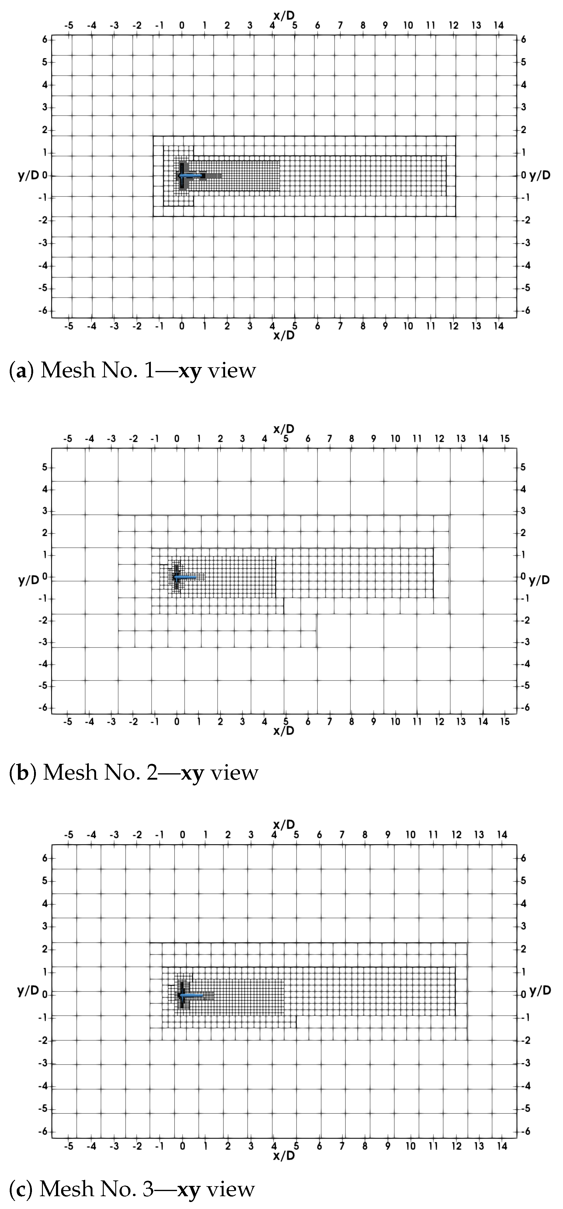
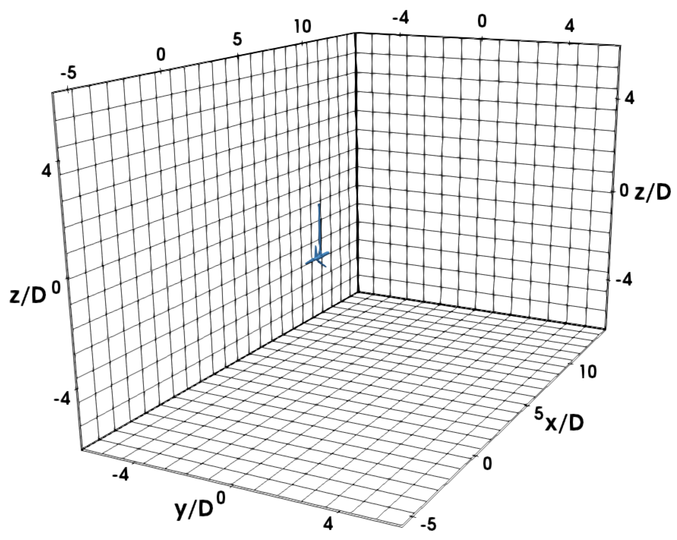
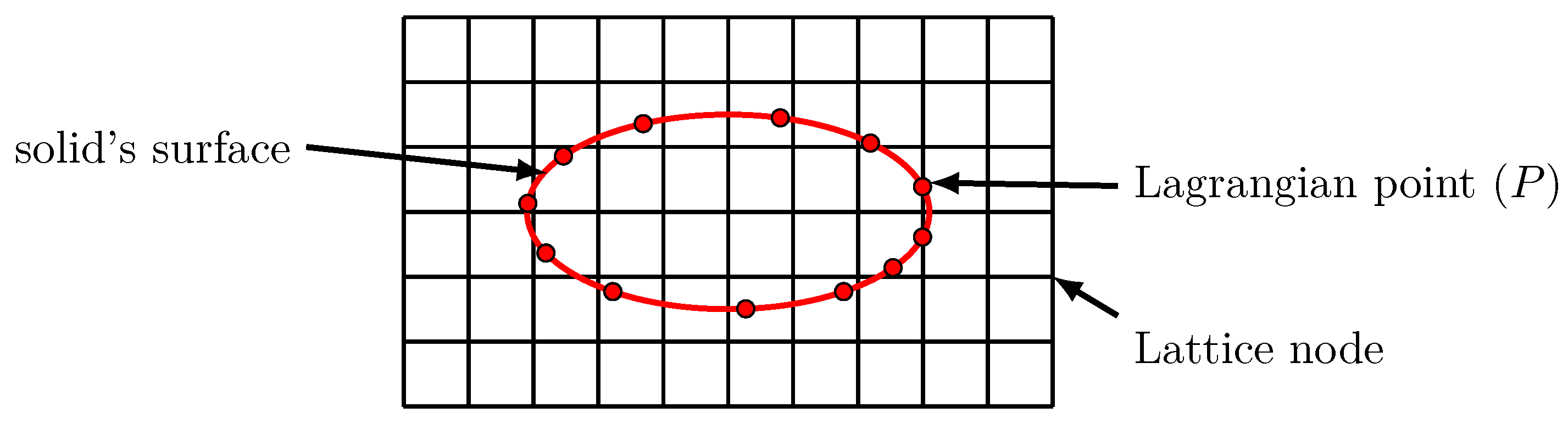
The LBM code used for this study works on a non-moving Cartesian mesh. A first comparison of the method with an NS-LES code has been made in [19]. The immersed boundary method (IBM) allows the modelling of complex geometries without any unstructured mesh fitting the geometry. The IBM is used here for modelling both the rotor and stator of the tidal turbine model. Ouro et al. [11] showed the capability of the IBM-NS to model the complex wake of vertical axis tidal turbine. Ouro et al. 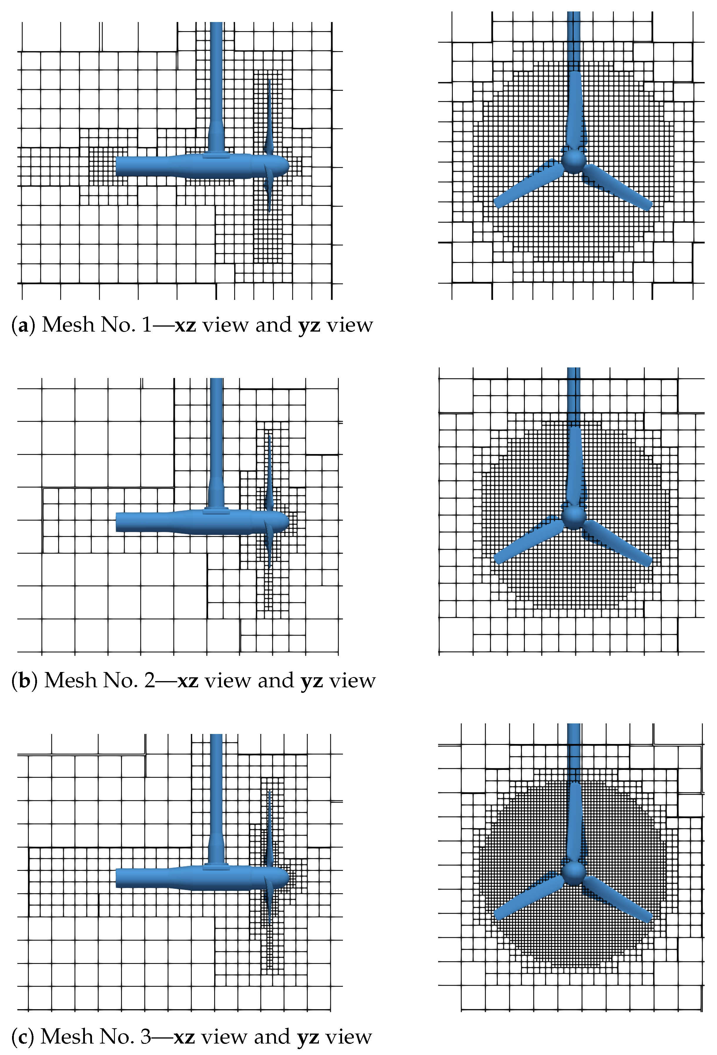[20] also used an IBM-NS model to predict the influence of turbulence on the loading of a tidal turbine. The use of a Cartesian mesh can be disadvantageous since it increases the number of nodes in the mesh. A multi-level Cartesian mesh is used [21]. This allows having smaller grid spacing in areas of interest such as in the wake or close to the turbine, thus reducing the total number of nodes.

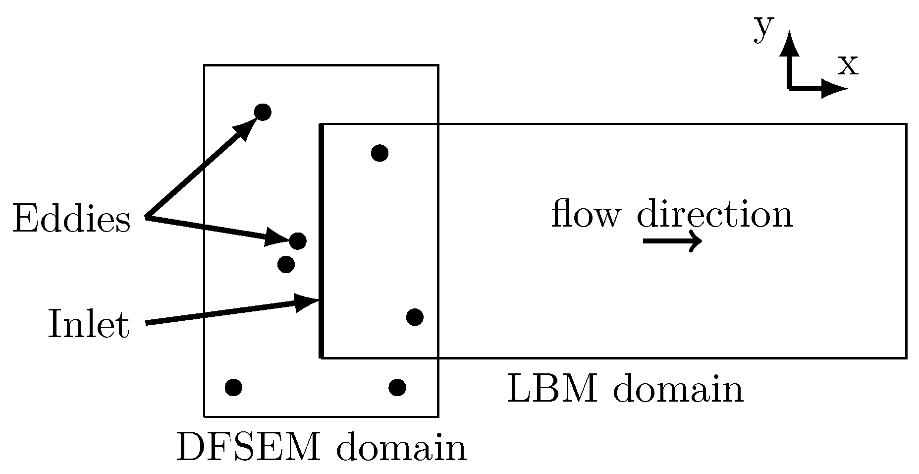
Turbulence intensity can vary from one site to another but it also varies along the tidal cycle of a specific site. Milne et al. [4] measured that the stream-wise turbulence rate varies between $7\%$ and more than $20\%$ along a cycle at the sound of Islay, Scotland. As the turbulence intensity varies significantly on a tidal site, it is important to know how a turbine reacts to several turbulence intensities. The influence of different turbulence intensities over quantities such as wake velocity and turbulence rate is investigated here. Upstream turbulence is generated with a divergence-free synthetic eddy method (DFSEM), introduced by Poletto et al. 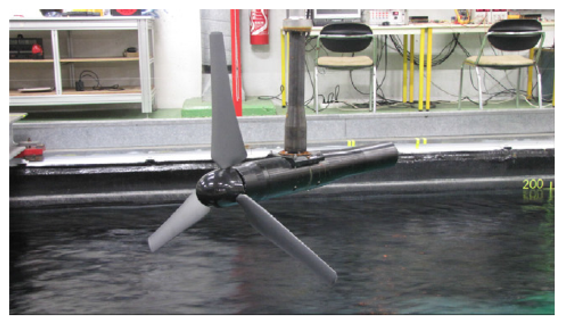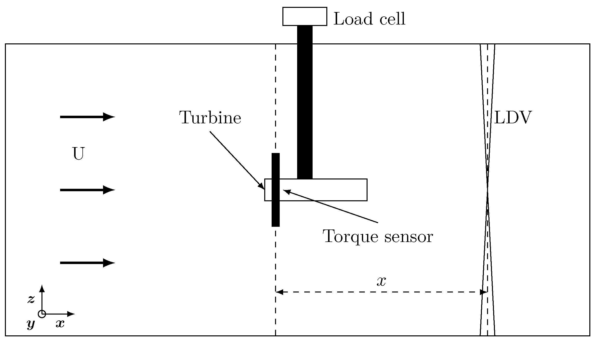[22]. The work presented in this paper aims at developing an LBM-LES tool to model tidal turbines in turbulent flows. This tool must be cheap enough to model several inflow configurations and turbine designs. This restriction is taken into account during the model setup. The case examined is a horizontal axis tidal turbine (HATT) model that was tested in Ifremer’s flume tank [6]. This case provides all the data required to validate the simulations at two turbulent rates, $3\%$ and $15\%$. Once the model is validated, a turbulent rate of $8\%$ is simulated. Simulations are performed with the open-source code Palabos.

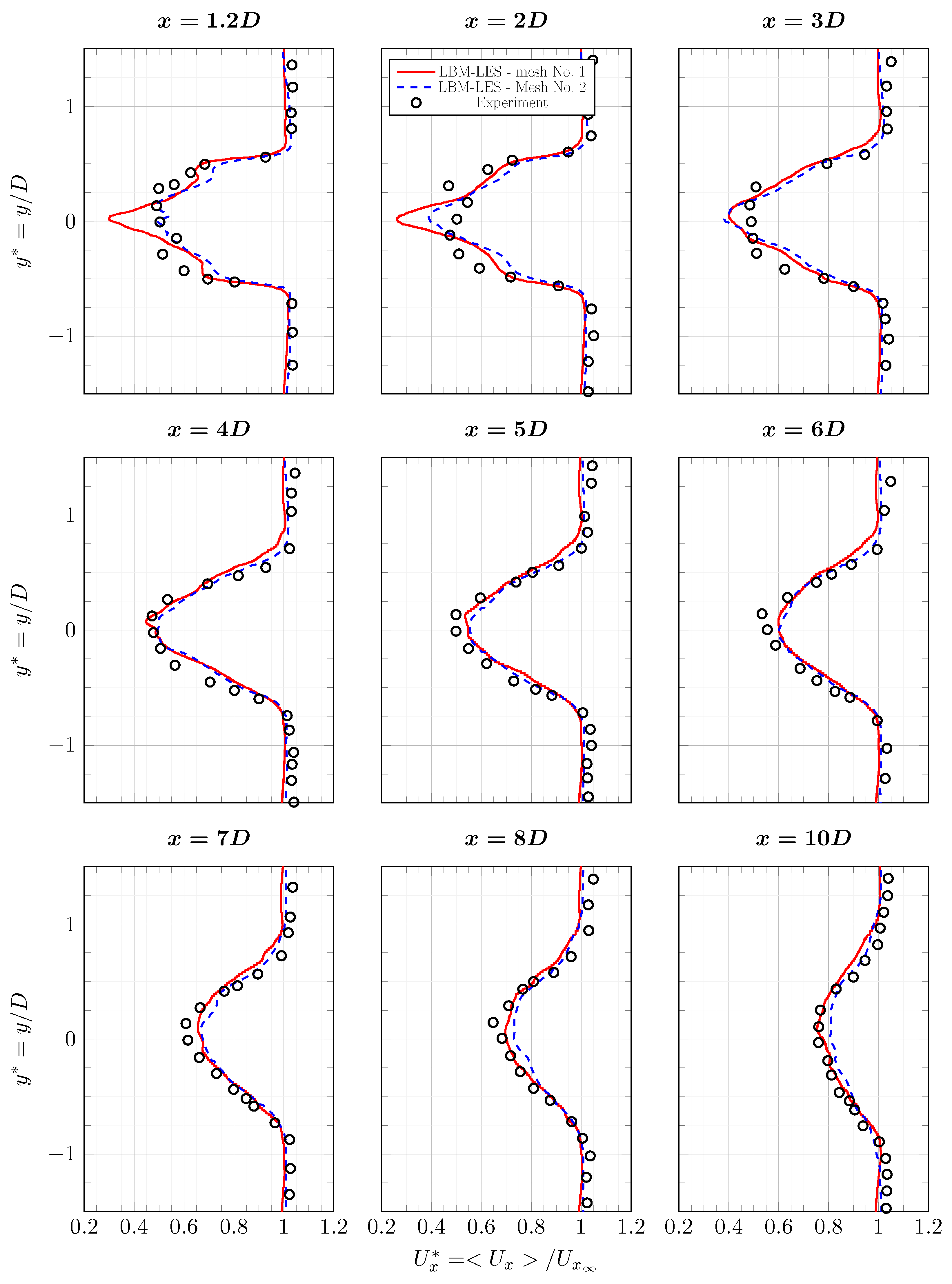
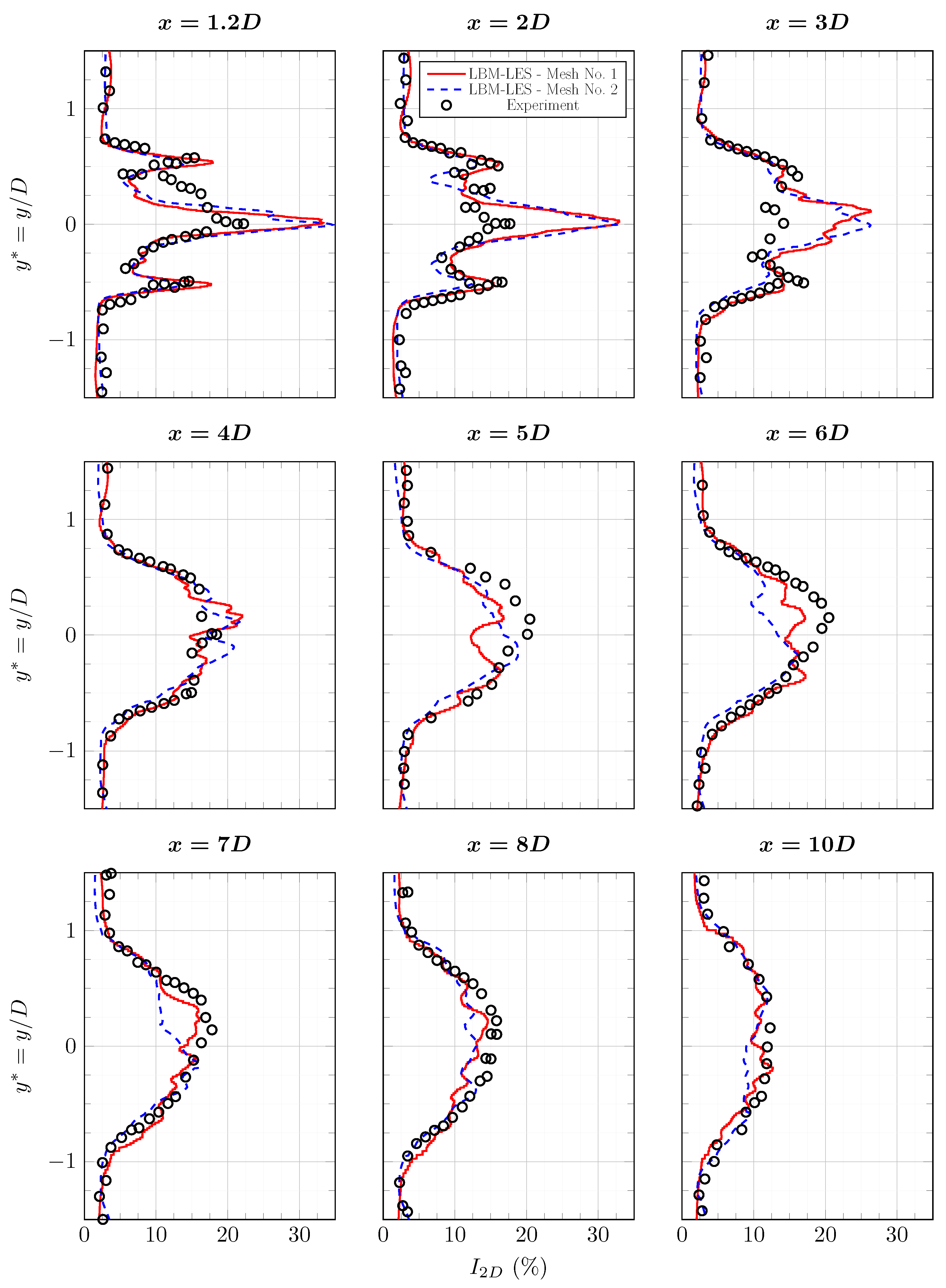
Section 2 describes the numerical and experimental set-up. Section 3 presents comparison of the model results with the experimental data from Mycek et al. In Section 4, the influence of the turbulence rate on the tidal turbine wake is investigated. Finally, Section 5 gives the conclusion and prospects of this study.

2. Materials and Methods

In this section, numerical methods and reference experiments are presented. The first part introduces the LBM and models chosen for this study. The experiment is then presented. The boundary conditions used to model the tidal turbine and the boundary conditions which generates inflow turbulence are presented in the third and fourth part. Finally, the numerical setup used to model the turbine is presented.

2.1. Lattice Boltzmann Method

The LBM is a numerical method that resolve the Boltzmann equation, Equation (1). It is an instationary weakly compressible method based on a statistical representation of the fluid through a density distribution function $f(\mathit{x},\mathit{\xi },t)$. This last represents the probability density for molecules being at a location $\mathit{x}$, which have the velocity $\mathit{\xi }$, at time t. The Boltzmann equation reads:

$$\frac{\partial f(\mathit{x},\mathit{\xi },t)}{\partial t}+\mathit{\xi }.\nabla f(\mathit{x},\mathit{\xi },t)=\Omega (f(\mathit{x},\mathit{\xi },t),f(\mathit{x},\mathit{\xi },t)),$$

(1)

where $\Omega$ is the collision operator and represents the collision between molecules. In the LBM, velocities $\mathit{\xi }$ are discretized using a predefined set of directions of propagation $c_i$ for molecules. A 2D example is given in Figure 1. Distribution functions are discretized according to these sets, giving the discrete partial distribution functions $f_i$. The method is implemented on a Cartesian lattice with temporal and spatial mesh width $\Delta t$ and $\Delta x$ of size 1.

The discretized Boltzmann equation is solved in two steps called collision and streaming. During the first one, post-collision distribution functions $f_i^{\prime }$ are computed using the collision operator $\Omega$. The second step is the streaming of post-collision distribution functions onto the neighbouring nodes pointed by the directions of propagation. Those two steps are illustrated in Figure 2 for a $D2Q9$ velocity scheme.

Macroscopic quantities of the fluid can be recovered using distribution functions. Density at a node is calculated with Equation (2) and velocity with Equation (3):

$$\rho =\sum _{i=0}^n{f}_i,$$

(2)

$$\rho \mathit{u}=\sum _{i=0}^n{c}_i{f}_i,$$

(3)

where n is the number of directions of propagation of the velocity scheme. Simulations presented in this study use a 3-dimensional set with 27 directions of propagation (D3Q27).

There are many collision operators. Simulations presented in this article are performed with a recursive and regularized collision operator (RR). The RR procedure was introduced by [23] to improve the stability and accuracy of the LBM. The collision operator is used with two-relaxation times (RR-TRT) and is available in Palabos under the name of Consistent Smagorinky Complete Regularized TRT dynamics. It is used at order 6. Boundary conditions use second-order accurate finite-difference approximations for velocity gradients scheme and can be used to apply velocity/pressure Dirichlet/Neumann conditions (Skordos [24]). This boundary condition is the most stable available in Palabos and is well suited for high Reynolds numbers simulations [25].

Uniform grids are not adapted to model complex geometries at high Reynolds numbers. To overcome this, static mesh refinement is used. The mesh refinement procedure is described in Lagrava et al. [21] and uses a multi-block approach. A convective scaling is set between various levels: $\Delta x_{coarse}=2\Delta x_{fine}$, $\Delta t_{coarse}=2\Delta t_{fine}$.

An LES approach is used and the subgrid model is a static Smagorinsky model [26]. It adds a turbulent viscosity calculated with Equation (4):

$${\nu }_{sgs}(\mathit{x},t)={(C_s^{\prime }\Delta x)}^2\left(2\right|\overline{S}(\mathit{x},t){{|}^2)}^{1/2},$$

(4)

where $\overline{S}$ is the filtered strain rate tensor. The implementation of the static Smagorinsky model in the LBM is described in Malaspinas and Sagaut [27]. The coefficient $C_s^{\prime }$ is linked to the Smagorinsky constant $C_s$ by using the Van Driest damping function, described in Equation (5), in order to cancel the turbulent viscosity close to the turbine’s surface. The distance normal to the surface is y, $\nu$ is the molecular viscosity of the fluid and $u_{\tau }$ is the friction velocity. The value $C_s=0.18$ has been chosen for this study.

$$C_s^{\prime }=C_s(1-exp\left(\frac{-y{u}_{\tau }}{26\nu }\right)).$$

(5)

2.2. Reference Experiment

The experiment as reference is the one of Mycek et al. [6]. He studied the wake and performances of a three-bladed tidal turbine model with two turbulent inflow conditions. The experiment has been carried out at Ifremer’s flume tank. The tidal turbine was developed by Ifremer and is illustrated in Figure 3. It is placed in the middle of the tank and the blockage ratio is approximately $4.8\%$.

Two turbulent inflow conditions were tested. The first one with $I=3\%$, where flow straighteners were used. The second one with $I=15\%$, where no flow straighteners were used. Several tip speed ratios (TSR) were also tested. The TSR of the numerical simulations is set close to the operating point at $TSR=3.67$. Characteristics chosen for the LBM-LES study are listed in

Table 1. Experimental configurations from Mycek et al. [6] studied with the LBM-LES.

Quantity	Value	Unit
Blade radius $R=D/2$	$0.35$	m
Flow velocity $<U_{x_{\infty }}>$	$0.8$	m.s${}^{-1}$
Tip speed ratio $TSR=\omega R/<U_{x_{\infty }}>$	$3.67$	~
Reynolds number $Re=<U_{x_{\infty }}>R/\nu$	$280\times {10}^3$	~
Turbulence intensity I	$\left[3,15\right]$	%

.

Performances of the turbine are evaluated with the thrust coefficient $C_T$ and power coefficient $C_P$, defined in Equations (6) and (7). $F_x$ is the axial force, $M_x$ the axial torque and $\omega$ the rotational speed of the rotor.

$$C_T=\frac{F_x}{0.5\rho \Pi R^2<U_{x_{\infty }}{>}^2}.$$

(6)

$$C_P=\frac{M_x\omega }{0.5\rho \Pi R^2<U_{x_{\infty }}{>}^3}.$$

(7)

The axial force is measured with a load cell placed at the fixing point of the turbine mast, so $F_x$ is the force applied to both stator and rotor. The torque is measured with a torque sensor located on the rotor axis. Wake measurements are made with laser Doppler velocimetry (LDV) and the frame origin is the rotor centre. The flow velocity $\mathit{U}$ and the location of the measurements x are presented in dimensionless units with ${\mathit{U}}^{*}=\mathit{U}/<U_{x_{\infty }}>$ and $x^{*}=x/R$. The experimental set-up is presented in Figure 4.

2.3. Modelling the Turbine

Boundary conditions for straight walls introduced in Section 2.1 are not adequate for modelling complex geometries like tidal turbines. Using such conditions would end with a staircase approximation of the surface and an inaccurate wake. The technique applied here is the immersed boundary method (IBM), which is well suited for modelling complex geometries [11]. The IBM was first introduced by Peskin [28] for simulating blood flow in the heart. The first use of IBM in an LBM simulation was done by Feng and Michaelides [29]. In Palabos IBM-LBM, the solid surface is discretized into a set of Lagrangian points. There should be enough points to correctly describe the solid and the spacing between points should not be superior to $\Delta x$. The IBM uses interpolations to compute the fluid velocity and density at each Lagrangian points P (Figure 5). Quantities are interpolated from lattice macroscopic quantities computed from pre-collision distribution functions. The solid boundary is modelled through a force acting on the fluid at the Lagrangian point’s location. The forcing method used in Palabos is based on [30]. The momentum at a Lagrangian point is written:

$${\rho }_P{\mathit{U}}_{boundary}={\rho }_P{\mathit{U}}_P+F_P,$$

(8)

where ${\mathit{U}}_{boundary}$ is the velocity of the boundary and $F_P$ is the forcing term. The force $F_P$ can be written: $F_P={\rho }_P({\mathit{U}}_{boundary}-{\mathit{U}}_P)$. The no-slip condition is then enforced by redistributing the force $F_P$ to the fluid momentum (Equation (9)):

$$\rho \left(\mathit{x}\right)\mathit{U}\left(\mathit{x}\right)=\rho \left(\mathit{x}\right)\mathit{U}\left(\mathit{x}\right)+\sum _P\tau S_P{F}_{P}D(\mathit{x}-{\mathit{x}}_{\mathit{P}}),$$

(9)

where S is the surface portion of the boundary represented by P and $D\left(\mathit{x}\right)$ is the Dirac distribution function. The relaxation frequency $\tau$ comes from the collision operator. This procedure is applied to every Lagrangian points of the boundary. The collision step is then executed with a modified momentum for the lattice nodes surrounding the Lagrangian points. More advanced IBM methods such as [31] could be explored in the future.

Simulating high Reynolds numbers flow with LBM-LES can be very resource consuming. Indeed, LES mesh size constraints at the wall are almost the same as direct numerical simulation (DNS) ones [32]. Using grid refinement helps but Cartesian meshes have many nodes compared to structured or unstructured meshes. To reduce the computational cost of simulations, a wall model is used. It is implemented using a pre-existing wall model of a beta version of Palabos. It is based on the model described in Ruffin et al. [33] and uses Spalding’s formulation of the boundary layer [34]:

$$y^{+}=u^{+}+e^{-\kappa B}\left[e^{\kappa u^{+}}-1-\kappa u^{+}-\frac{{\left(\kappa u^{+}\right)}^2}{2}-\frac{{\left(\kappa u^{+}\right)}^3}{6}\right],$$

(10)

where $y^{+}$ is the normalized distance to the solid surface: $y^{+}=u_{\tau }y/\nu$. The velocity $u^{+}$ is calculated with: $u^{+}=U/u_{\tau }$. The variable $\kappa$ is the von Kármán constant and B is a constant. The Newton–Raphson method is used for computing $u_{\tau }$. The turbulent viscosity is computed like in Ruffin et al. [33] and applied to the lattice by modifying the relaxation time like in Malaspinas and Sagaut [35]. Spalding’s law of the wall needs two parameters: $\kappa$ and B. For the simulations presented thereafter, $\kappa =0.42$. The parameter B can slightly vary depending on the mesh size or the upstream turbulence, it is typically equal to $B=2.6\pm 0.2$.

2.4. Generating Realistic Inflow Conditions

There are several ways of implementing a realistic turbulent inflow condition. In Grondeau et al. [36], the synthetic eddy method (SEM) developed by Jarin et al. [37] has been implemented in Palabos. The SEM generates a random turbulent inflow condition that matches a specified average Reynolds tensor and average axial velocity. It gave good results at low Reynolds numbers. As the Reynolds number increases, simulations can become unstable due to density fluctuations generated by the SEM boundary condition. To overcome this issue, the divergence-free SEM (DFSEM) of Poletto et al. [22] has been implemented in Palabos and is used here. The DFSEM is closed to the SEM except for the calculation of velocity fluctuations. The algorithm can be summarized by the following steps:

(1)

Definition of the DFSEM parameters: average stream-wise velocity $<U>$, eddy length L, Reynolds tensor, number of eddies N;

(2)

Creation of the eddy box around the inlet of the LBM domain, see Figure 6;

(3)

Creation of N eddies at a random location and with random intensities;

(4)

Displacement of eddies in the stream-wise direction;

(5)

Computation of eddies contributions to the fluctuations of the average stream-wise velocity;

(6)

Repeat 4 and 5.

When an eddy is leaving the DFSEM domain it is deleted. A new eddy is created at $x=0$ in the DFSEM reference frame with random $y,z$ positions and intensities. Each eddy adds velocity fluctuations to the surrounding inlet nodes. The radius of an eddy influence zone is defined by the eddy length L. Fluctuations are computed using Equation (11).

$$u_{node}^{\prime }=\sqrt{\frac{1}{N}}\sum _{k=1}^N\frac{q_L\left(\right|{\mathit{r}}_k)|}{|{\mathit{r}}_k{|}^3}{\mathit{r}}_k\times {\alpha }_k,$$

(11)

where $q_L$ is the shape function and ${\mathit{r}}_k=\frac{\mathit{x}-{\mathit{x}}_k}{L}$, with $\mathit{x}$ the position of the node and ${\mathit{x}}_k$ the position of an eddy. The shape function used is defined in Equation (12).

$$q_L\left(a\right)=\sqrt{\frac{16V_B}{15\pi L^3}}sin{\left(\pi a\right)}^{2}a,$$

(12)

where $V_B$ is the volume of the DFSEM domain. Polleto et al., (2013) suggested to use an eddy density d around 1 in order to have a good compromise between computational cost and accuracy. The eddy density is define in Equation (13).

$$d=\frac{L^{3}N}{V_B}.$$

(13)

The DFSEM boundary condition is applied through the Dirichlet boundary condition of Palabos. The objective is to generate synthetic turbulence as close as possible to the turbulence of Mycek et al.’s [6] experiment. In addition to the data provided by Mycek et al. [6], an analysis of the upstream and downstream turbulence was made by Medina et al. [38]. The general definition of the turbulence intensity, noted I or $I3D(\%)$, is based on the three components of the velocity fluctuations, and is given by Equation (14), where $<u_i^{{}^{\prime }2}>$ are the time-averaged velocity fluctuations and $<U_i>$ are the time-averaged velocity components. In addition, the stream-wise turbulence intensity $I1D(\%)$ is based on the velocity component in the current direction. Similarly, the two-dimensional turbulence intensity $I2D(\%)$ is based on the velocity fluctuation in the flow direction and in the transverse direction. The turbulence rates $I_{1D}$ and $I_{2D}$ are defined in equation Equations (15) and (16). Measured turbulence rate I, $I_{1D}$ and $I_{2D}$ were also provided by Ifremer. Depending on the source, the turbulence rate I is found between $12.5\%$ and $15\%$ for the case where no flow straighteners are used. According to those sources, the turbulence rate is constant in the stream-wise direction. When using a synthetic turbulent inflow condition, one should verify that the turbulence intensity is conserved over a long enough distance. Indeed, for a high turbulence rate, the artificial turbulent structures rapidly lose their intensity and the turbulence rate decreases according to the stream-wise direction. Accordingly, we choose to generate a flow with a turbulence rate of $I=12.5\%$. This case is denominated “$I=12.5\%$” from now on. When flow straighteners are used, the turbulence rate is close to $I=3\%$. This value is kept for this study and this case is denominated “$I=3\%$”.

$$I=I_{3D}=100\sqrt{\frac{1/3(<u_x^{{}^{\prime }2}>+<u_y^{{}^{\prime }2}>+<u_z^{{}^{\prime }2}>)}{<U_x{>}^2+<U_y{>}^2+<U_z{>}^2}}$$

(14)

$$I_{1D}=100\sqrt{\frac{<u_x^{{}^{\prime }2}>}{<U_x{>}^2}}$$

(15)

$$I_{2D}=100\sqrt{\frac{0.5(<u_x^{{}^{\prime }2}>+<u_y^{{}^{\prime }2}>)}{(<U_x{>}^2+<U_y{>}^2)}}$$

(16)

The study made by Medina et al. [39] has brought to light that the turbulence of the flume tank is fully developed. The length scale of turbulent structures was estimated to be between $0.25$ m and $0.6$ m for $I=12.5\%$ and between $0.65$ m and $0.9$ m for $I=3\%$. The turbulence is isotropic for $I=12.5\%$, whereas for $I=3\%$, the stream-wise velocity fluctuation is stronger than the other two components. The implemented DFSEM does not allow strong anisotropy ratios and the velocity fluctuations are smoothed over the three directions.

The DFSEM is used to generate a realistic inflow boundary condition. The implemented DFSEM needs four parameters to work: the convection velocity of the DFSEM eddies, the number of DFSEM eddies, the size of DFSEM eddies and the imposed Reynolds tensor. The velocity of the DFSEM eddies is equal to the average upstream stream-wise velocity $<U_{x_{\infty }}>$. To define the number of eddies, Polleto et al. (2013) suggested using an eddy density d around 1 in order to have a good compromise between computational cost and accuracy. The eddy density is defined in Equation (13). It is chosen to $d=1$ for the case with $I=3\%$. For the case with $I=12.5\%$, the eddy density is chosen to be $d=2$ to avoid spatial disparity. The size of DFSEM eddies and the imposed Reynolds tensor are chosen carefully after dedicated studies, presented in Section 3.1. Those studies are carried out without the turbine in order to save computational resources. It allows for longer simulated durations, enabling advanced statistics like spatial autocorrelation. For those studies, the numerical domain is 4 m high, 4 m wide and 12 m long. The mesh is uniform and, unless stated otherwise, $\Delta x=0.035$ m.

2.5. Setup of the Turbine Modelling

This subsection introduces the numerical domains used for modelling the turbine presented in Section 2.2. In order to have elements regarding the mesh sensitivity of the approach, three mesh configurations are studied. The static mesh refinement of Palabos is used here. The three meshes are summarized in

Table 2. Meshes selected for the LBM mesh sensitivity study. The finest level is the numerical domain surrounding the rotor of the turbine. $h.CPU$ is the wall-clock time multiplied by the number of CPU used.

Mesh	Finest Level	$\mathbf{\Delta }\mathit{x}$ at Finest Level	Number of Nodes Revolution in h.CPU	Computational Time Per
No. 1	6	$1.39\times {10}^{-3}$ m	$83\times {10}^6$	$450$ h.CPU
No. 2	6	$1.04\times {10}^{-3}$ m	$60\times {10}^6$	$1300$ h.CPU
No. 3	5	$7.32\times {10}^{-4}$ m	$124\times {10}^6$	$1910$ h.CPU

. The boundary layer model used is only valid in the logarithmic layer, viscous sub-layer and buffer layer [33]. Therefore, the coarsest mesh is chosen in order to have a $\Delta x_{max}^{+}\approx 300$ for $TSR=3.67$. The finest level of the mesh has the highest number and the coarsest level has level number 0.

Meshes around the turbine are shown in Figure 7. Only the area swept by the rotor is refined at the finest level. Indeed, the flow around the blades is the area where the Reynolds number is the highest and where the boundary layer is the thinnest. The finest mesh volume for mesh No. 2 and 3 is much smaller than for mesh No. 1. After running simulations with mesh No. 1, it seemed impractical to use the same finest mesh volume for mesh No. 2 and 3. In order to lower the computational cost, considerable work has been done to lower as much as possible the number of nodes in the finest domain. Since convective scaling is used, all three cases are run with a constant Mach number of $Ma=0.38$.

Full meshes are visible in Figure 8. The turbine is located more than $5D$ downstream of the inlet. Considering the small blockage ratio, the flume tank is not modelled and the turbine is $6D$ away from lateral boundaries. The wake is divided into two areas, the close wake up to $4D$ and the far wake from $4D$ and up to $11.5D$. Because of how the mesh refinement works in Palabos, the mesh size in the wake of the three cases is slightly different.

Table 3. Mesh sizes in the wake of the turbine.

Mesh	Close Wake Level	$\mathbf{\Delta }\mathit{x}$ Close Wake	Far Wake Level	$\mathbf{\Delta }\mathit{x}$ Far Wake
No. 1	3	$5.58\times {10}^{-3}$ m	2	$11.16\times {10}^{-3}$ m
No. 2	3	$8.30\times {10}^{-3}$ m	2	$16.60\times {10}^{-3}$ m
No. 3	3	$5.58\times {10}^{-3}$ m	2	$11.16\times {10}^{-3}$ m

summarizes the mesh size in the wake of the turbine. Liu and Hu [40] studied the turbine of Mycek et al. [6] with an ALM unsteady-RANS model. A converged solution have been obtained with a mesh size in the wake of $8.75\times {10}^{-3}$ m. This is slightly larger than the wake mesh size of Mesh No 2. A three-dimensional view of the domain is shown in Figure 9.

The Dirichlet boundary condition modified with DFSEM is used on the inlet and with $\mathit{U}=(<U_{x_{\infty }}>,0,0)$ on sides boundaries. The outlet is a pressure-imposed boundary condition. On every boundary, except for the inlet, a pressure-wave absorbing function is applied to distribution functions. This function is described in Xu and Sagaut [41]. Simulations are carried out at the Centre Régional Informatique et d’Application Numérique de Normandie (CRIANN, France) on Broadwell CPU cores ($2.4$ GHz).

3. Inlet Calibration and Validation

This section first presents the results of the study dedicated to the choice of DFSEM parameters. The chosen sets of DFSEM parameters are then used for the LBM-LES modelling of the turbine. Results of those simulations are presented afterwards.

3.1. Upstream Turbulence for the Tidal Turbine

The choice of DFSEM parameters is first investigated for the case with $I=3\%$ and then for the case with $I=12.5\%$. Stream-wise evolutions of quantities such as turbulence rate, power spectral density or integral length scale are investigated.

3.1.1. DFSEM, Low Upstream Turbulence Rate Case (I = 3%)

For this case, the choice of parameters is straightforward. The size of eddies is $L=1.0$ m, which is close to the maximum of the measured integral length scale ${\mathcal{L}}_{max}=0.9$ m. L is equal to the diameter of eddies since they are sphere shaped. The Reynolds tensor is chosen as a diagonal matrix and all diagonal terms are equal: $u_x^{{}^{\prime }2}=u_y^{{}^{\prime }2}=u_z^{{}^{\prime }2}=8.928\times {10}^{-4}$ m${}^2$.s${}^{-2}$.

Figure 10 shows the evolution of the turbulence rate $I_{1D}$ according to the stream-wise direction. The turbulence rate is almost conserved along the flume tank. An autocorrelation function is used to compute the integral length scale $\mathcal{L}$ of turbulent structures. This function is applied in the plane of normal $\mathit{z}$ at $z=2$ m and according to the direction $\mathit{y}$. It is defined in Equation (17):

$$AC\left(\mathit{x}\right)=\frac{3}{N_{AC}(<u_x^{{}^{\prime }2}>+<u_y^{{}^{\prime }2}>+<u_z^{{}^{\prime }2}>)}\sum _{i=0}^{N_{AC}}\mathit{U}\left(\mathit{x}\right).U\left({\mathit{x}}_0\right),$$

(17)

where $N_{AC}$ is the number of iterations during which the autocorrelation is applied. The point ${\mathit{x}}_0$ is located at the centre of the domain. Figure 11 shows the evolution of the estimated integral length scale according to the stream-wise direction.

The integral length scale of turbulent structures generated by the DFSEM boundary condition is conserved along the stream-wise direction and is close to the prescribed eddy length L.

Turbulent flows are complex phenomena where coherent structures of several scales evolve. Large structures are the most energetic and energy goes from big structures to small structures. This energy cascade is observable with a power spectral density (PSD) calculated from a sampling of the velocity. The PSD from a developed turbulent flow has a slope of $-5/3$, characteristic of the energy cascade. The stream-wise velocity component is recorded at the centre of the flume at $f=112$ Hz in $x=2.0,4.0$ and $9.0$ m. The PSD calculated from this recording is plotted in Figure 12.

A drop in the PSD for frequencies higher than 1 Hz is observed. This drop has two origins: only big structures are generated by the DFSEM boundary condition and the relatively coarse mesh does not allow for small structures to be conserved. The PSD would certainly be closer to the $-5/3$ slope with a finer mesh but the volume upstream of the turbine is too big for a finer mesh size. For the frequencies inferiors to 1 Hz, the PSD is close to the $-5/3$ slope.

To conclude, the turbulent flow generated with the DFSEM is close to the experimental flow upstream of the turbine for $I=3\%$. The chosen set of parameters is: $u_i^{{}^{\prime }2}=8.928\times {10}^{-4}$ m${}^2$.s${}^{-2}$ and $L=1.0$ m. Those parameters are used to model the tidal turbine with the LBM-LES with $I=3\%$ in Section 3.2.1.

3.1.2. DFSEM, High Upstream Turbulence Rate Case (I = 12.5%)

The turbulent flow generated by the DFSEM loses its intensity as it travels in the flume. This effect increases with the turbulence rate. Consequently, the choice of parameters is less straightforward for high inflow turbulence rates and several sets of parameters must be tested. Three sizes of eddies are tested: $L=0.25,0.66$ and $1.2$ m. Two Reynolds tensors are tested. They are both diagonal and diagonal terms are equal to: $u_x^{{}^{\prime }2}=u_y^{{}^{\prime }2}=u_z^{{}^{\prime }2}=0.01638$ and $0.04000$ m${}^2$.s${}^{-2}$. Two mesh sizes are tested: $\Delta x=0.035$ and $0.025$ m. The evolution of the turbulence rate $I_{1D}$ according to the stream-wise direction, for several sets of parameters, is plotted in Figure 13.

In cases where L is equal to $0.25$ m and $0.6$ m both, have a strong decay of the turbulence rate. The eddy size seems to have a great influence on the decay of the turbulence rate. Cases with $u_i^{{}^{\prime }2}=0.01638$ m${}^2$.s${}^{-2}$ and $u_i^{{}^{\prime }2}=0.04000$ m${}^2$.s${}^{-2}$ converge toward the same turbulence rate. Increasing the velocity fluctuations at the inlet is not a solution. A finer mesh size does not have a significant influence on the decay of the turbulence rate. It appears that the best solution to conserve a high enough turbulence rate is to increase the size of eddies.

The autocorrelation function used previously is applied to the case with $L=1.2$ m. Results are plotted in Figure 14. The estimated integral length scale is conserved and close to the prescribed size of eddies. Following Blackmore et al. [42] and Ebdon et al. [12] the turbulence integral length scale has a great influence on the behaviour of the turbine. Because the prescribed size L is conserved in the canal, a compromise must be chosen. The set $L=1.2$ m and $u_i^{{}^{\prime }2}=0.01638$ m${}^2$.s${}^{-2}$ allows conserving the turbulence rate above $10\%$. This set is chosen for the case $I=12.5\%$. Since L is twice as large as $\mathcal{L}$, this set of parameters may induce some discrepancies.

Table 4. Turbulence rates from a LBM-LES simulation using DFSEM with $L=1.2$ m, $u_i^{{}^{\prime }2}=0.01638$ m${}^2$.s${}^{-2}$ and $\Delta x=0.025$ m. x is the distance from the inlet of the LBM domain. Turbulence rates are calculated at the centre of the LBM domain.

x (m)	${\mathit{I}}_{1\mathit{D}}(\%)$	${\mathit{I}}_{2\mathit{D}}(\%)$	${\mathit{I}}_{3\mathit{D}}(\%)$
$0.1$	$13.00$	$12.76$	$12.88$
$2.0$	$12.65$	$12.28$	$12.25$
$6.0$	$10.34$	$10.06$	$9.98$
$9.0$	$8.25$	$8.11$	$8.13$
Slope	$-0.547$	$-0.533$	$-0.543$

presents the evolution of the turbulence $I_{1D}$, $I_{2D}$, and $I_{3D}$ defined in Equations (14)–(16). The slope linear regression through the data points employed in [43,44] was used to estimate the rate of change in the distance from the inlet of the LBM domain with turbulence rates. It was observed that as the distance from the inlet of the LBM domain increases, $I1D(\%)$ decreases at the rate of $-0.547$, $I2D(\%)$ decreases at the rate of $-0.533$, while $I3D(\%)$ decreases at the rate of $-0.543$. Rates at which the 1D, 2D and 3D turbulence intensities decreases are extremely close, which tends to indicate that the turbulence generated by the DFSEM is isotropic.

The PSD of the stream-wise velocity is plotted in Figure 15. Close to the inlet, a drop is observed at the frequency of DFSEM eddies. This drop quickly disappears and the slope of the PSD converges toward the $-5/3$ slope around $x=4.0$ m.

To conclude, a compromise has been made in order to conserve the turbulence rate over a long enough distance. The chosen set of parameters is: $u_i^{{}^{\prime }2}=0.01638$ m${}^2$.s${}^{-2}$ and $L=1.2$ m. A distance of convergence of approximately 4 m has been observed. The turbine location, presented in Section 2.5, respects this conclusion.

3.2. Tidal Turbine Modelling

Results from the LBM-LES simulations of the turbine are presented here, at first with a low upstream turbulence rate, then with a high upstream turbulence rate. Simulations results are compared with experimental results, investigated wake quantities are the average axial velocity and the average turbulence rate. Force coefficients from simulations are also compared to experimental ones.

3.2.1. Turbine, Low Upstream Turbulence Rate Case (I = 3%)

The simulation of the tidal turbine, described in Section 2.2, with an upstream turbulence rate of $I=3\%$ is performed with an LBM-LES code. Quantities in the wake and force coefficients are averaged over 12 s at a sampling rate of 398 Hz. A convergence duration of 16 s is respected before the calculation of average quantities.

Table 5. Turbine force coefficients from [6] and from LBM-LES simulations at $TSR=3.67$ and $I=3\%$. Differences are calculated between the experiment and simulations.

Mesh	${\mathit{C}}_{\mathit{T}}$	Difference	${\mathit{C}}_{\mathit{P}}$	Difference
Experiment	$0.805$	∖	$0.420$	∖
No. 1	$0.74$	$-7.8\%$	$0.50$	$19.7\%$
No. 2	$0.79$	$-1.2\%$	$0.48$	$13.5\%$
No. 3	$0.82$	$1.4\%$	$0.46$	$9.1\%$

presents force coefficients from both the experiment and simulations. It appears that mesh No. 2 and 3 are converged in thrust coefficient $C_T$. Mesh No. 1 gives a relatively good $C_T$ prediction with an error of less than $10\%$. The difference in power coefficient $C_P$ keeps decreasing with the mesh size. Nevertheless, the error in $C_P$ is always lower than $20\%$, which is relatively good considering the fact that the boundary layer is not fully resolved. Mesh No. 2 is a compromise between accuracy and computational cost. For the rest of the study, simulations are carried out with mesh Nos. 1 and 2. Mesh No. 1 is kept because it cost three times less than mesh No. 2 and may give good wake prediction.

Average axial velocity profiles and turbulence intensity profiles are plotted in Figure 16 and Figure 17. At $1.2D$ downstream of the turbine, in the close wake, the difference between LBM-LES simulations with mesh No. 1 and mesh No. 2 is non-negligible. The average axial velocity is better calculated with mesh No. 2. The interaction between the mast and the wake creates an asymmetry of the wake and is visible on the experimental turbulence profile at $x=1.2D$. This asymmetry is not on the simulations profiles. This interaction is probably not properly computed by the boundary layer model. The turbulence peak around $y=\pm 0.5D$ is correctly predicted by both LBM-LES simulations, it is most probably coming from tip-vortices. Tip-vortices can be observed in Figure 18. After $2D$, both the axial velocity and the turbulence intensity are correctly calculated by LBM-LES simulations with mesh Nos. 1 and 2. On the turbulence profile obtained with mesh No. 1, a small irregularity is observed $5D$ downstream of the turbine. Considering the shape of this irregularity, it may come from the tip-vortices. This could indicate that either the tip-vortices have slightly different behaviour in this simulation, or the quantities are not averaged over a duration long enough.

3.2.2. Turbine, High Upstream Turbulence Rate Case (I = 12.5%)

The simulation of the tidal turbine described in Section 2.2 with an upstream turbulence rate of $I=12.5\%$ is performed with an LBM-LES code. As stated in Section 3.2.1, LBM-LES simulations are only carried out with mesh No. 1 and 2. Quantities in the wake and force coefficients are averaged over 16 s at a sampling rate of 398 Hz. It is slightly more than for $I=3\%$ because a higher turbulence rate requires a longer sampling duration. Convergence lasts 16 s.

Table 6. Turbine force coefficients from [6] at $TSR=3.67$ and $I=12.5\%$ and from LBM-LES simulations at $TSR=3.67$ with $I=12.5\%$.

Mesh	${\mathit{C}}_{\mathit{T}}$	Difference	${\mathit{C}}_{\mathit{P}}$	Difference
Experiment	$0.73$	∖	$0.37$	∖
No. 1	$0.70$	$-4.4\%$	$0.462$	$23.0\%$
No. 2	$0.75$	$3.4\%$	$0.48$	$28.6\%$

shows force coefficients from the LBM-LES simulations and experiment. Mesh Nos. 1 and 2 give good thrust predictions. However, they both overestimate the power coefficient and gives relatively close power predictions. It has been pointed out in Section 3.1 that the chosen size of eddies could induce discrepancies. Indeed, Blackmore et al. [42] have observed that increasing the integral length scale could increase force coefficients. This could explain the observed differences in $C_P$.

Average axial velocity profiles and turbulence intensity $I_{2D}$ profiles are plotted in Figure 19 and Figure 20. Differences are small between the two meshes, except at $1.2D$ where the average axial velocity is a bit more accurate with mesh No. 2. At $1.2D$ downstream, a slight shift of the wake in the y direction is observed on the experimental profile. Data provided by Ifremer show that the upstream flow is not perfectly uni-axial when no flow straighteners are used. A small $\mathit{y}$ component exists and may affect the direction of propagation of the wake. It could explain the difference. Except for this difference, the axial velocity profiles from the simulations are close to the experimental ones.

The maximum turbulence intensity predicted by the LBM-LES simulation is identical to the experimental one. There is a lack of turbulence elsewhere in the close wake. For instance, in the $-1<y^{*}<1$ interval at $x=1.2D$, the average experimental $I_{2D}$ intensity is $22\%$, whereas it is $16\%$ in the simulation with mesh No. 1. There is no obvious explanation for this difference but several sources may be suggested. The boundary layer model may react badly to the high rate of upstream turbulence or the integral length scale may influence the production of turbulence. This difference decreases in the far wake. Despite not being revealed through a located peak on averaged profiles, tip-vortices are observed in Figure 21. The ambient turbulence’s influence is seen to be notable as tip-vortices rapidly lose consistency.

The LBM-LES simulations have proven to be reliable to predict the wake of tidal turbines with a high upstream turbulence intensity. A more detailed study of the wake is proposed in the next section.

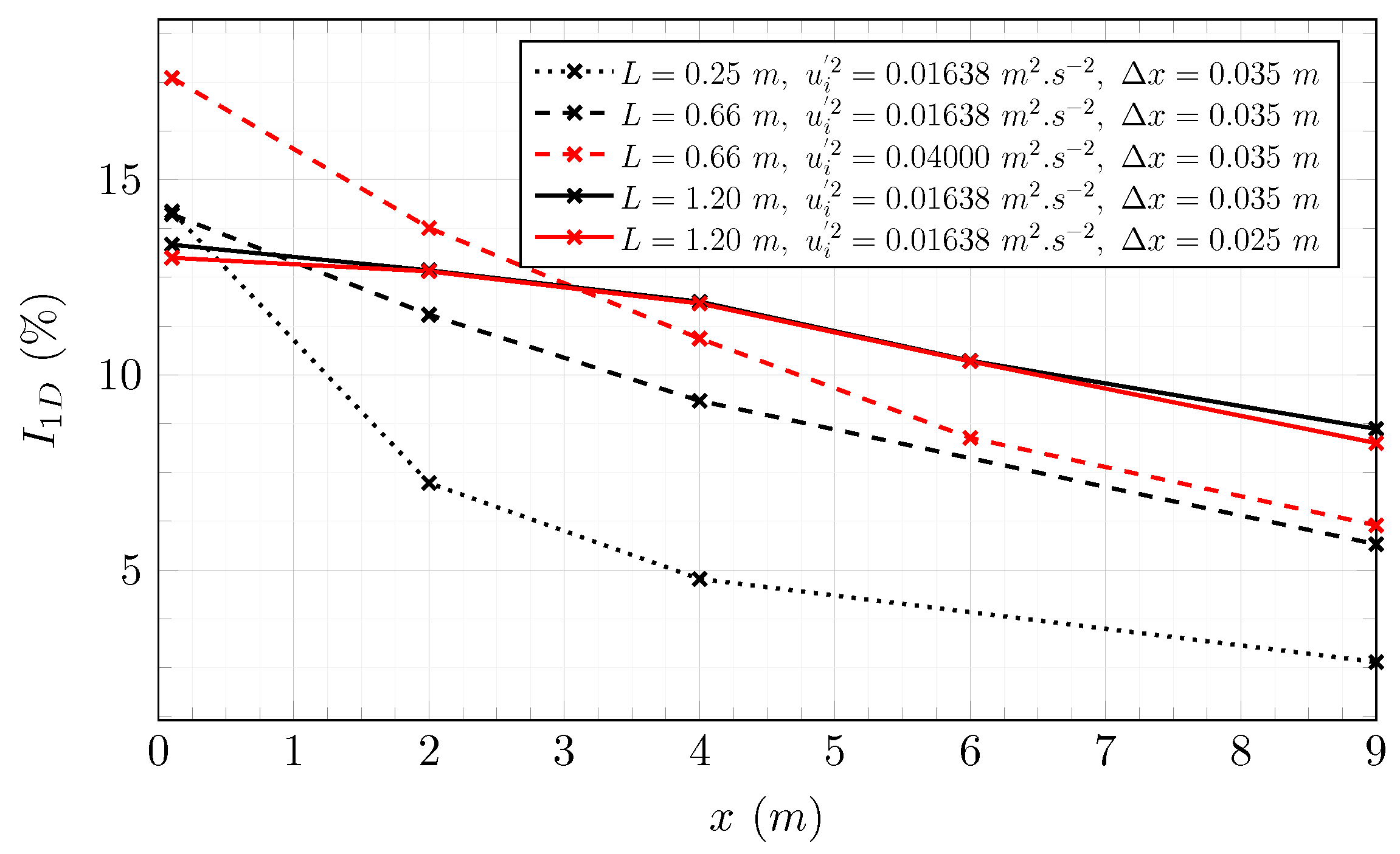
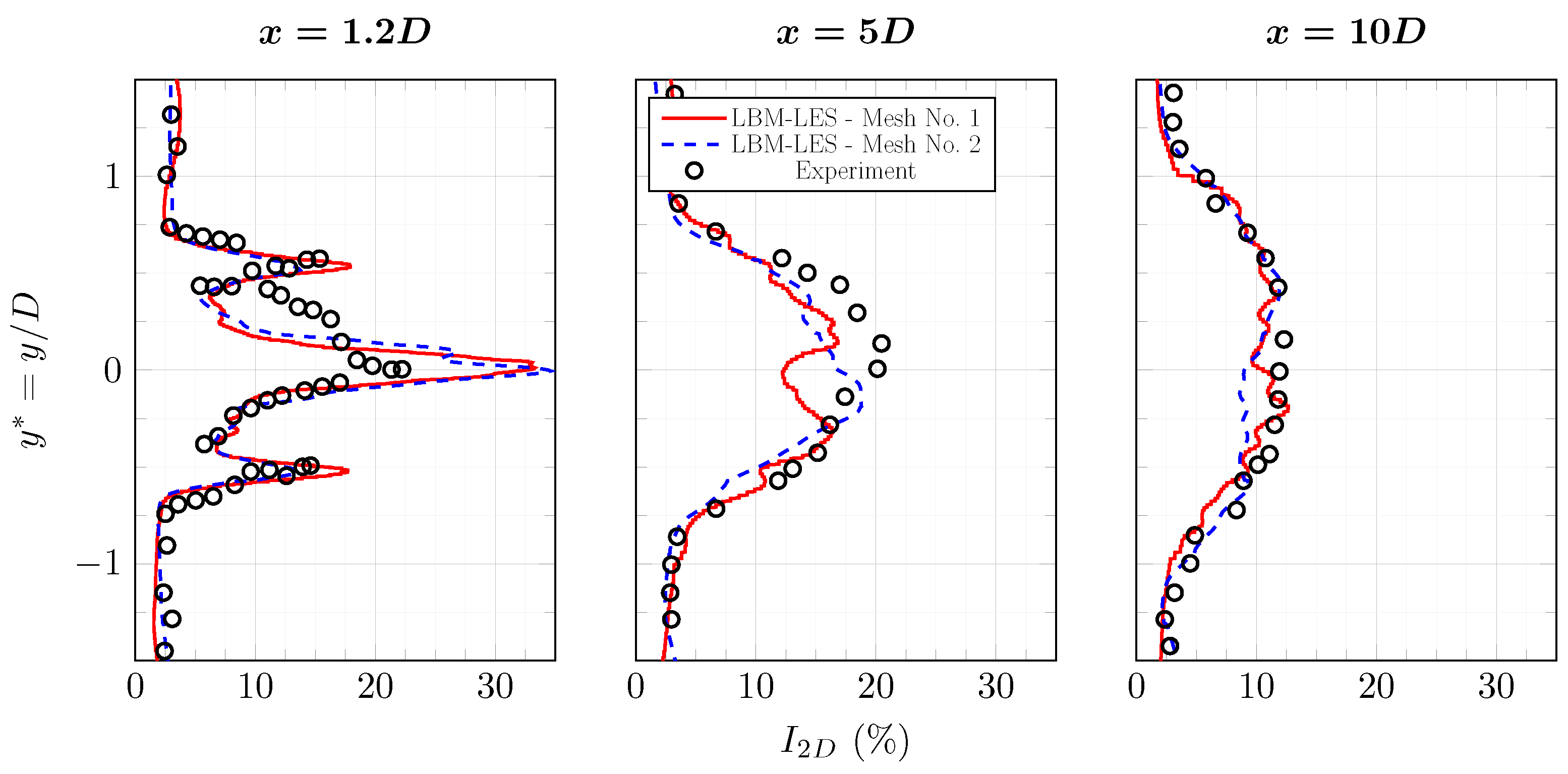
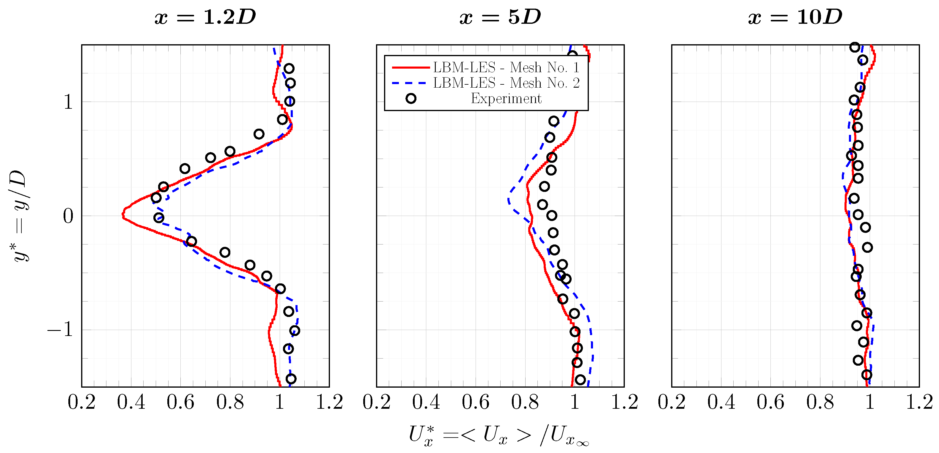
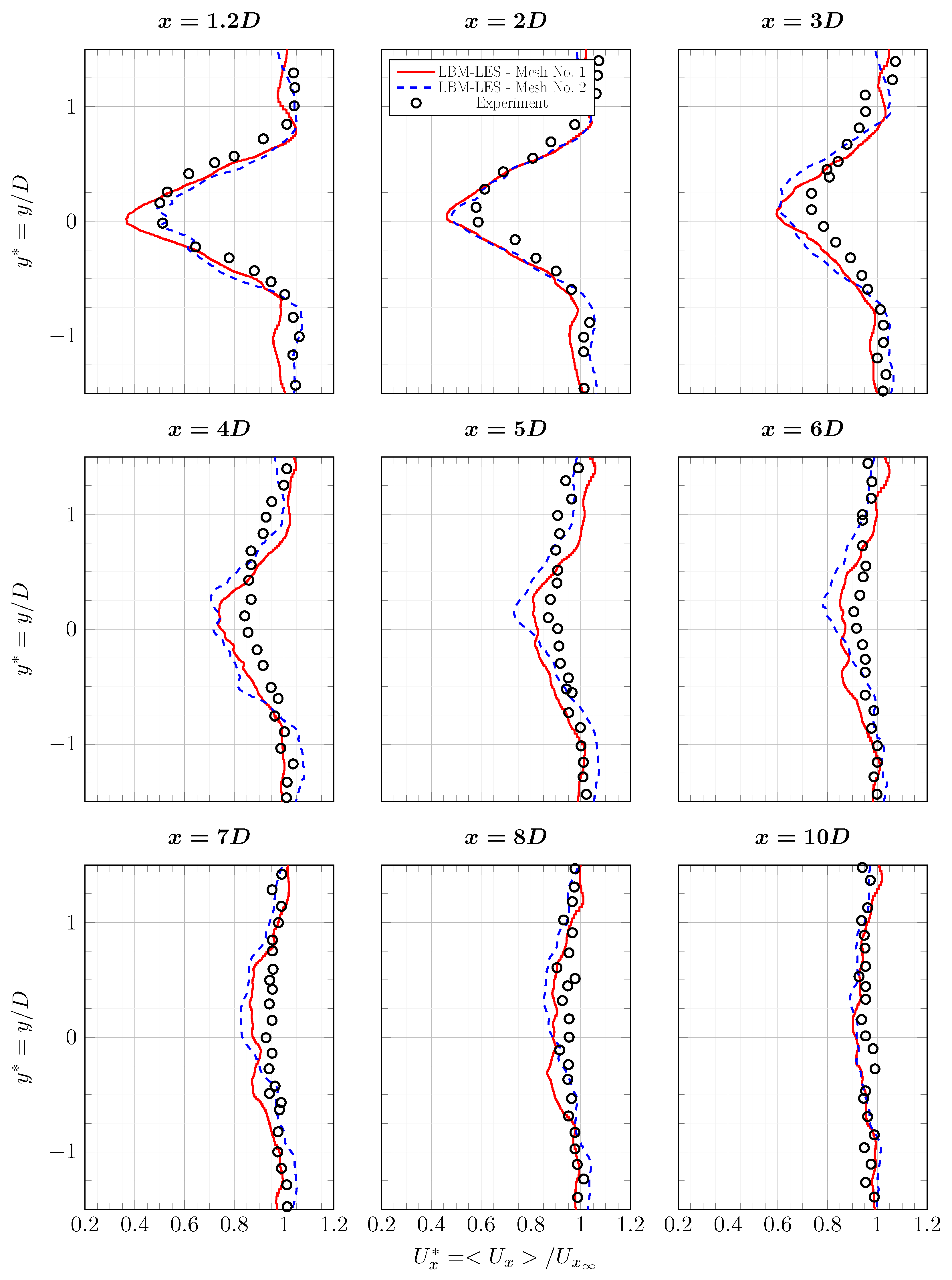
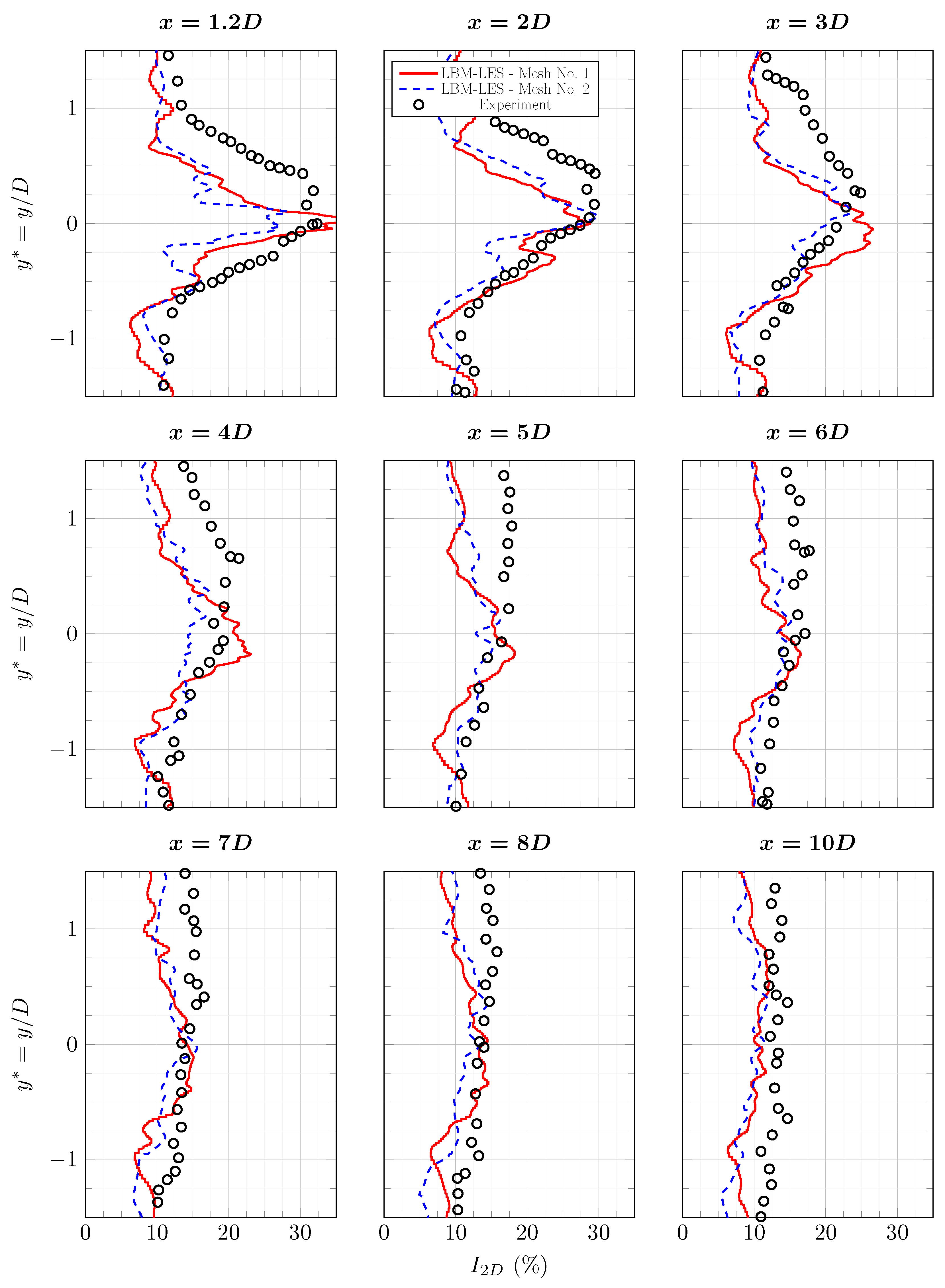
4. Wake Analysis

Velocity deficit and increase of turbulence have been observed in turbines’ wake. Thus, previous results have shown that the upstream turbulence has a great influence over the wake of a tidal turbine. In this section, a cross-comparison between simulations at I = 3, 8 and 12.5% is carried out. Then a spectral analysis is proposed. Finally, the propagation of tip-vortices is studied. A third LBM-LES simulation with an upstream intensity of I = 8% is realized. This turbulence intensity has been observed in different areas favourable to tidal stream facilities [3]. Except for the upstream turbulence, this simulation is identical to the simulation with an upstream turbulence intensity of I = 12.5%.

4.1. Cross-Comparison

A comparison based on the averaged axial velocity, the average turbulence rate and the average shear stress is proposed here. Quantities from the case at $I=8\%$ are obtained with the same procedure as for the case at $I=12.5\%$.

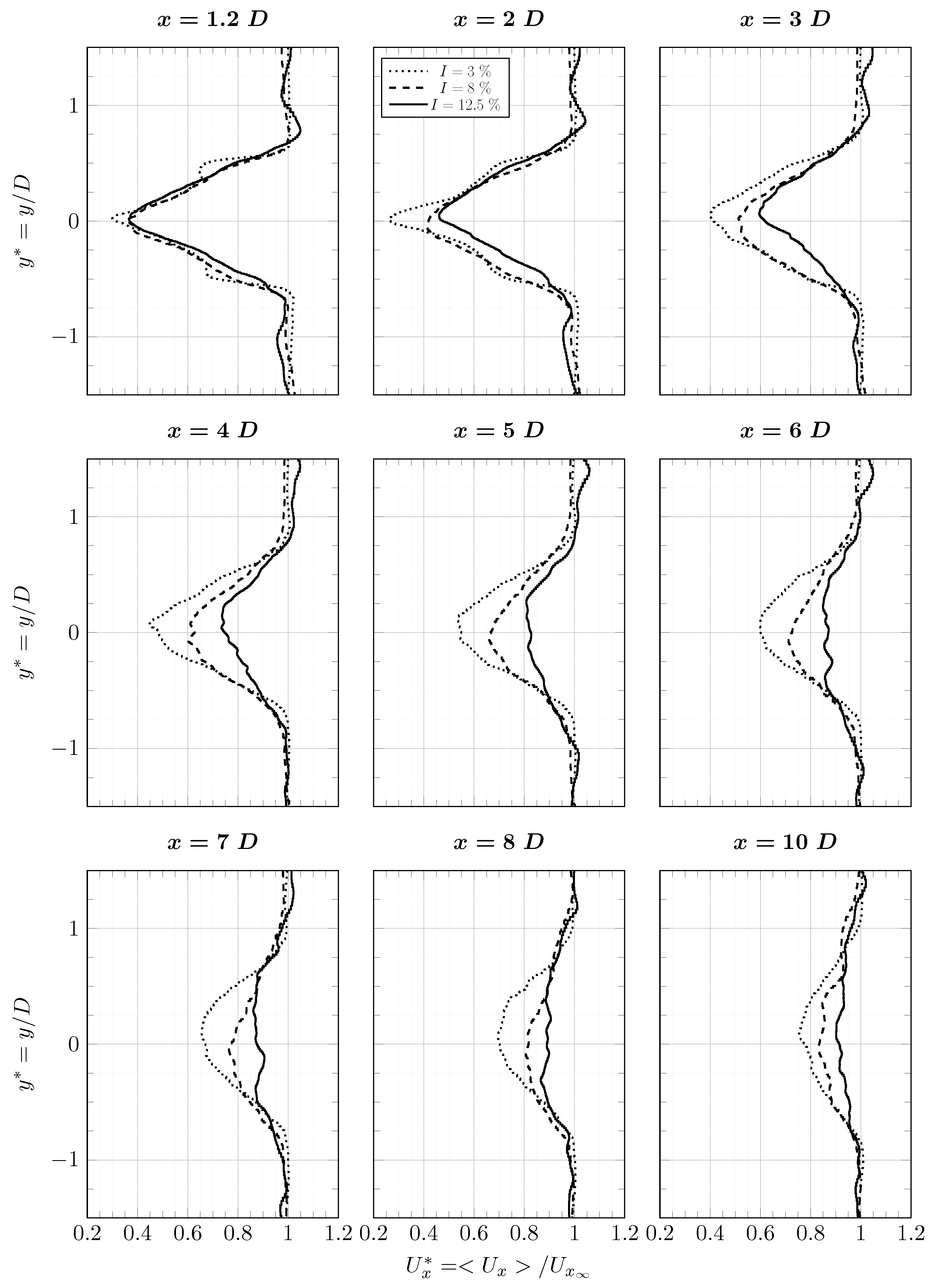
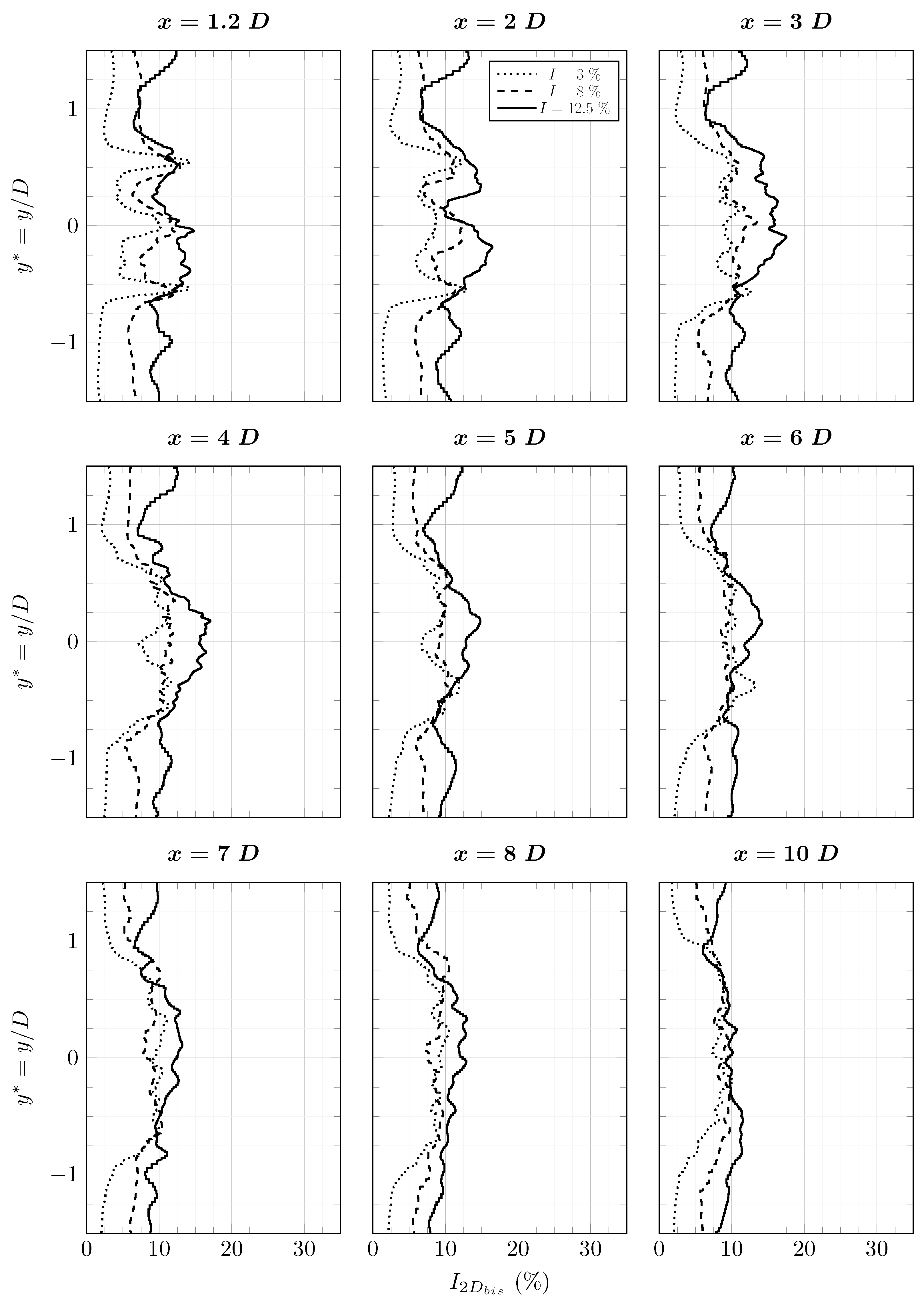
The axial velocity in the wake has a different evolution according to the upstream turbulence rate (Figure 22). The turbine footprint is still visible on the average axial velocity profile of the simulation at $I=8\%$ at $x=10D$. The axial velocity $<U_x>$ for the simulation at $I=8\%$ is always included between the axial velocity of the simulations at $I=3\%$ and $I=12.5\%$. The turbulence rate $I_{2D_{bis}}$ in the wake is plotted in Figure 23 and is defined in Equation (18):

$$I_{2D_{bis}}=100\sqrt{\frac{0.5(<u_x^{{}^{\prime }2}>+<u_y^{{}^{\prime }2}>)}{<U_{x_{\infty }}{>}^2}}.$$

(18)

The wake, observed with the quantity $I_{2D_{bis}}$, can be divided into three zones. A first zone from $x=0D$ to $x=5D$ where the turbulence rate $I_{2D_{bis}}$ is different for the three cases and increases with the upstream turbulence rate. A second zone between $x=5D$ and $x=9D$ is observed. In this zone, the turbulence rates $I_{2D_{bis}}$ of cases at $I=3\%$ and $I=8\%$ are equal. The turbulence rate $I_{2D_{bis}}$ from the case $I=12.5\%$ is greater. A third zone at $x=10D$ can be identified. In this zone, the turbulence rate $I_{2D_{bis}}$ is the same for all three cases. 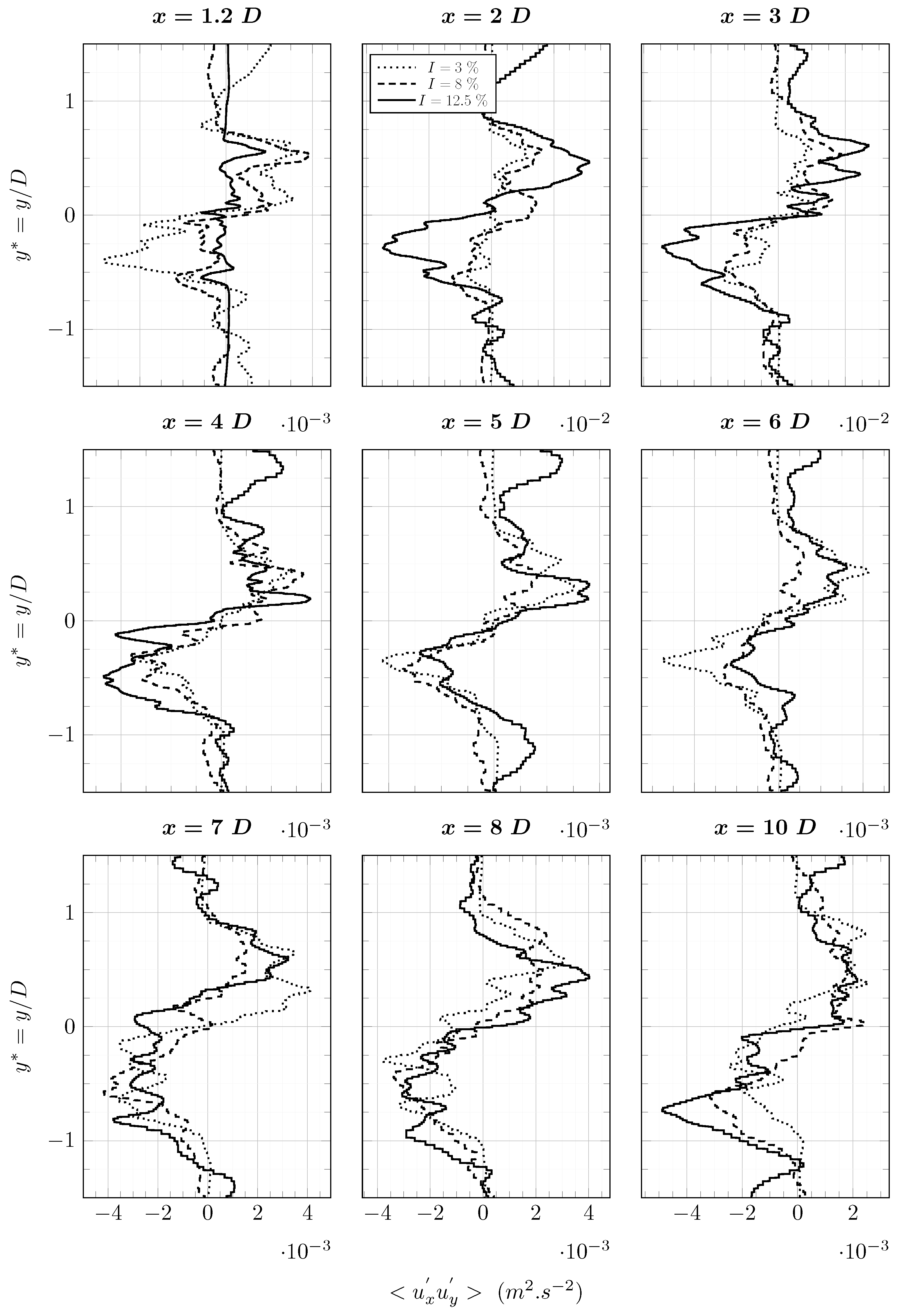The shear stress $<u_x^{{}^{\prime }}{u}_y^{{}^{\prime }}>$ has a different behaviour (Figure 24). From $x=6D$ to $x=10D$, the shear stress is very close for all three cases. However, the lack of samples makes observations difficult.

The diameter of the wake can be estimated from the axial velocity profiles (Figure 22). It is calculated assuming that the averaged axial velocity profiles are close to a Gaussian distribution. The diameter of the wake can be estimated as $D_w=(6/1.177)y_{1/2}$, where $y_{1/2}$ is the half-width of the profile at $<U_x>=(<U_{x_{\infty }}>+<U_{x_{min}}>)/2$. The calculated $D_w$ are summarized in

Table 7. Diameter of the wake of tidal turbine at $TSR=3.67$ calculated from averaged axial velocity profiles from LBM-LES simulations with upstream turbulence intensities of $I=\left[3,8,12.5\right]\%$.

Upstream Turbulence	Diameter at $\mathit{x}=4\mathit{D}$	Difference	Diameter at $\mathit{x}=5\mathit{D}$	Difference	Diameter at $\mathit{x}=7\mathit{D}$	Difference
$3\%$	$1.23$ m	∖	$1.33$ m	∖	$1.50$ m	∖
$8\%$	$1.57$ m	$+28\%$	$1.61$ m	$+21\%$	$2.07$ m	$+38\%$
$12.5\%$	$1.54$ m	$-2\%$	$2.13$ m	$+32\%$	$2.41$ m	$+16\%$

. The diameter of the wake increases according to the $\mathit{x}$ direction. It is wider for high upstream turbulence rates. Those observations are in agreement with the observations made by [6].

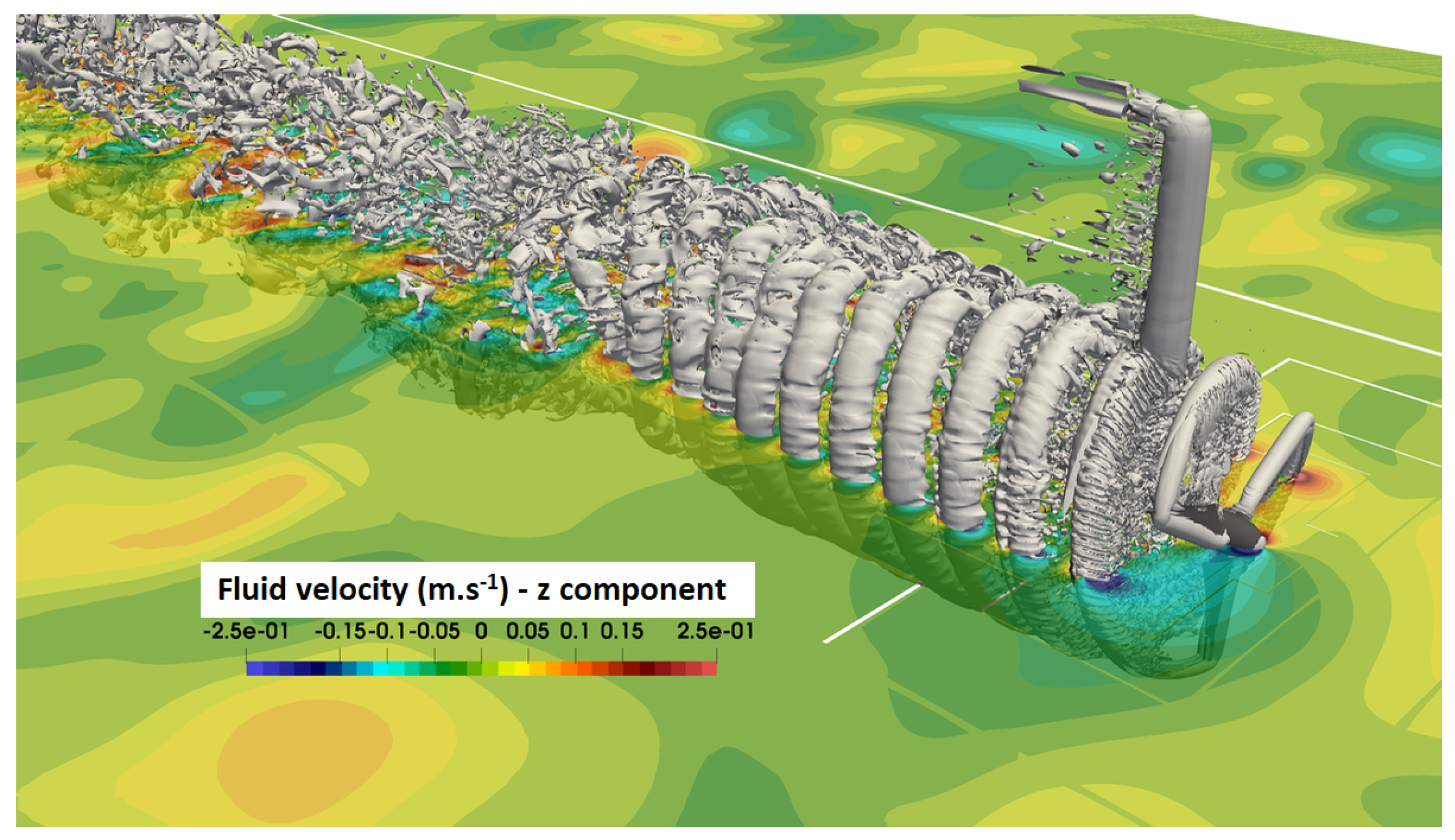
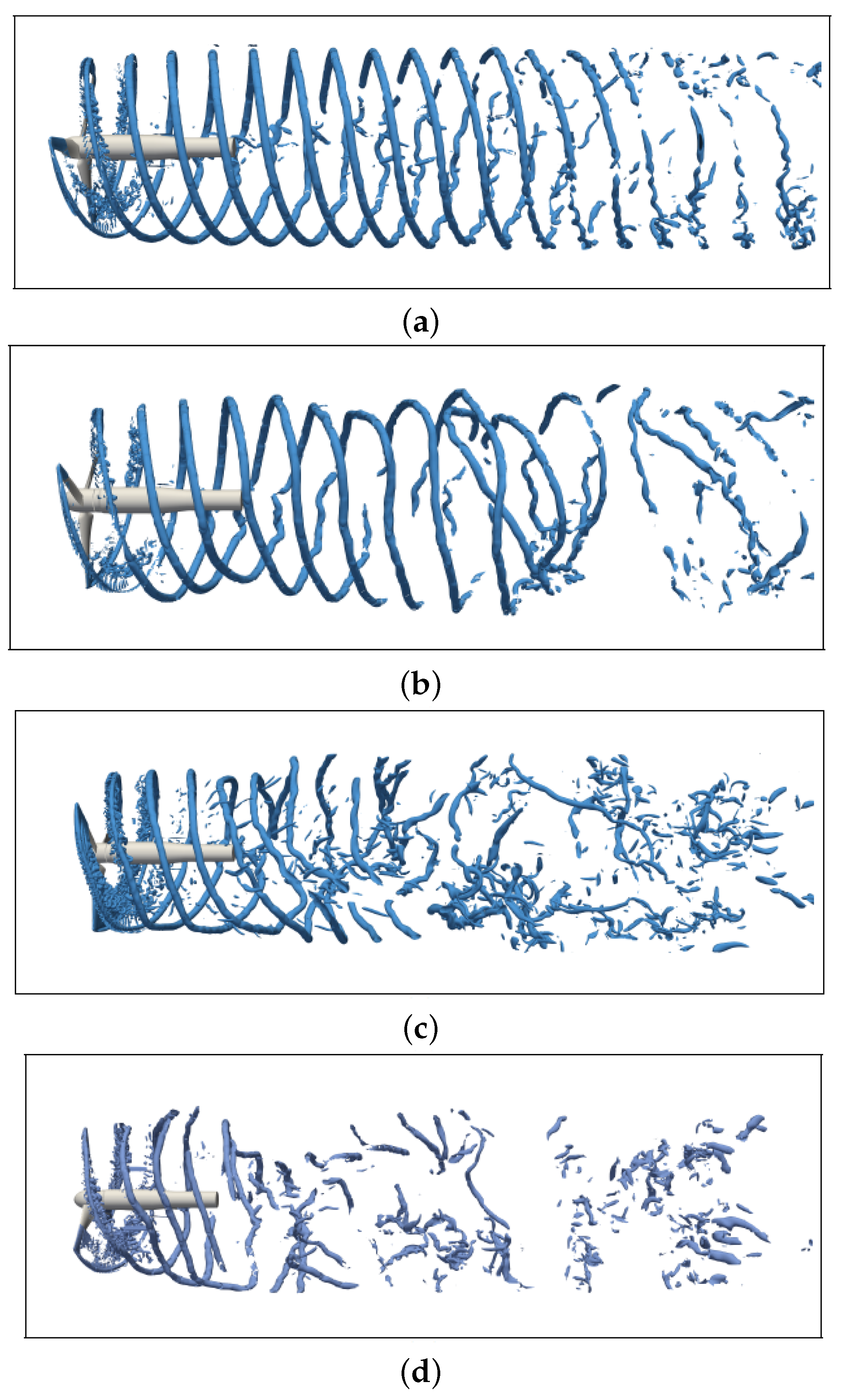
Iso-surfaces of the ${\lambda }_2$ criterion are shown in Figure 25. The ${\lambda }_2$ criterion was introduced by Jeong and Hussain [45] to identify the centre of turbulent structures in turbulent flows. More details about this criterion and others can be found in Kolár [46]. Only iso-surfaces included between $R=0.15$ m and $R=0.42$ m are shown in Figure 25. The iso-surface of ${\lambda }_2$ criterion is shown with no upstream turbulence in Figure 25a and with upstream turbulence $I=3\%$ in Figure 25b. The tip-vortices are visible on both figures. Tip-vortices are coherent turbulent structures with high energy. They are one of the main sources of turbulence in the wake. Studying their propagation is important for wake prediction. The upstream turbulence has an influence on the propagation of those structures. It seems to affect their envelope and the duration during which they are coherent.

Tip-vortices with an upstream turbulence of $I=8\%$ can be observed in Figure 25c and with $I=12.5\%$ in Figure 25d. They are highly disrupted by the upstream turbulence. Snapshots of the wake can hardly provide information about the propagation of turbulent structures such as tip-vortices.

Even if only average quantities of the wake are considered, it is difficult to predict a priori the evolution of the wake as a function of the upstream turbulence. The average velocity deficit on the rotation axis seems to have a linear behaviour whereas it is hard to perceive a pattern for average fluctuations and tip-vortices. The next two analyses bring some elements in order to have a better understanding of the phenomena that take place in the wake.

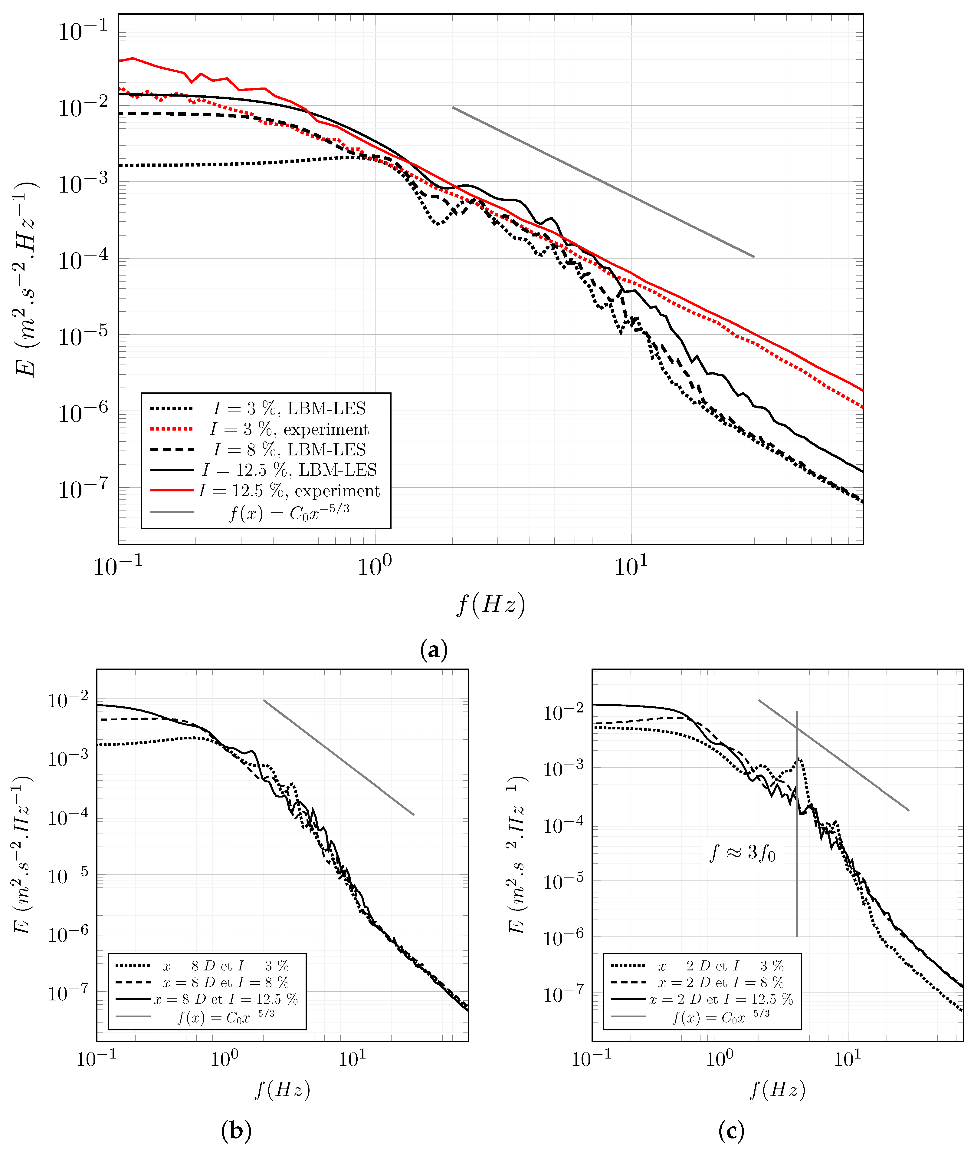
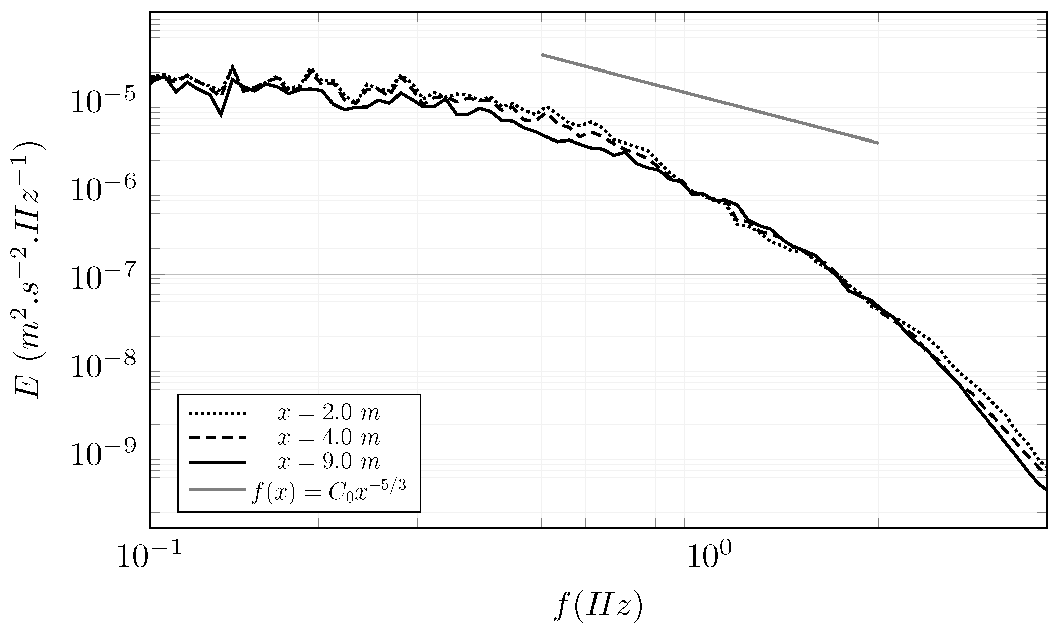
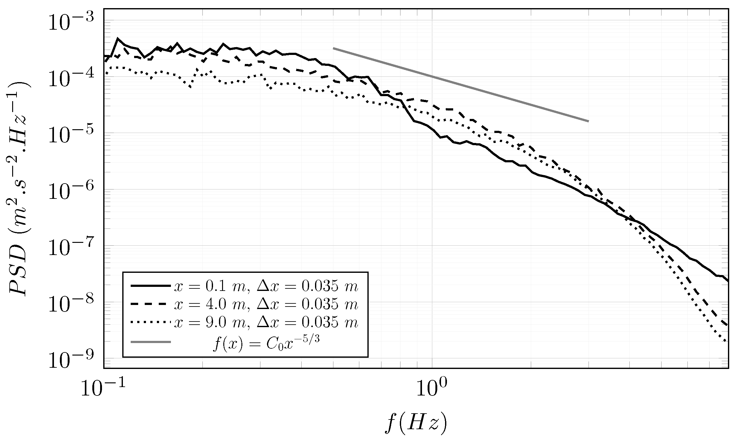
4.2. Spectral Analysis

Experimental spectral data in the wake of the tidal turbine are available in Medina et al. [38]. They used the same turbine as the one simulated here but at $TSR=4.0$.

Figure 26a compares LBM results with the experiment made by [38]. Power spectral density (PSD) computed from the LBM simulation with an upstream turbulence rate of $12.5\%$ is close to the experimental one up to 10 Hz frequency. After 10 Hz, the energy of the PSD from the LBM simulation drops below the experimental one. Numerical dissipation and mesh size, $\Delta x=5.58\times {10}^{-3}$ m, are the main cause of this difference. PSD from the simulation with $I=3\%$ is further away from the experiment. The PSD from the LBM simulation with $I=8\%$ is included between the $I=3\%$ PSD and $I=12.5\%$ PSD, which could be expected. It can be observed that it is closer to the $I=3\%$ PSD. A similar observation was made with $I_{2D_{bis}}$ in the previous section.

Far from the turbine at $x=8.0D$ (Figure 26b), PSD of the three cases are quite similar. This observation and the observations made in the cross-comparison suggest that the turbulence in the wake converge toward a state independent from the upstream turbulence intensity. It is to be noted that none of the chosen upstream turbulence rates exceed the turbulent rates calculated at $x=10D$ downstream of the turbine.

Figure 26c shows the PSD calculated from the axial velocity in the wake at $y=R$. A peak is observed on the PSD from the case $I=3\%$ at the frequency $3f_0$. The frequency $f_0=1.335$ Hz is the rotating frequency of the rotor. This peak is not present on the PSD from the cases $I=\left[8,12.5\right]\%$. There are two explanations. Either the tip-vortices have already lost their consistency or they are too much disrupted to be observed at a given location.

The PSD from the simulations has been found to be quite reliable compared to the experimental PSD. Some observations have been made regarding the evolution of the turbulence in the wake. It has been suggested that the turbulence converges toward a state independent from the upstream turbulence. The chosen spectral approach is not suited to observe the evolution of some specific structures like tip-vortices. A spatial approach is proposed hereafter to analyse the propagation of tip-vortices.

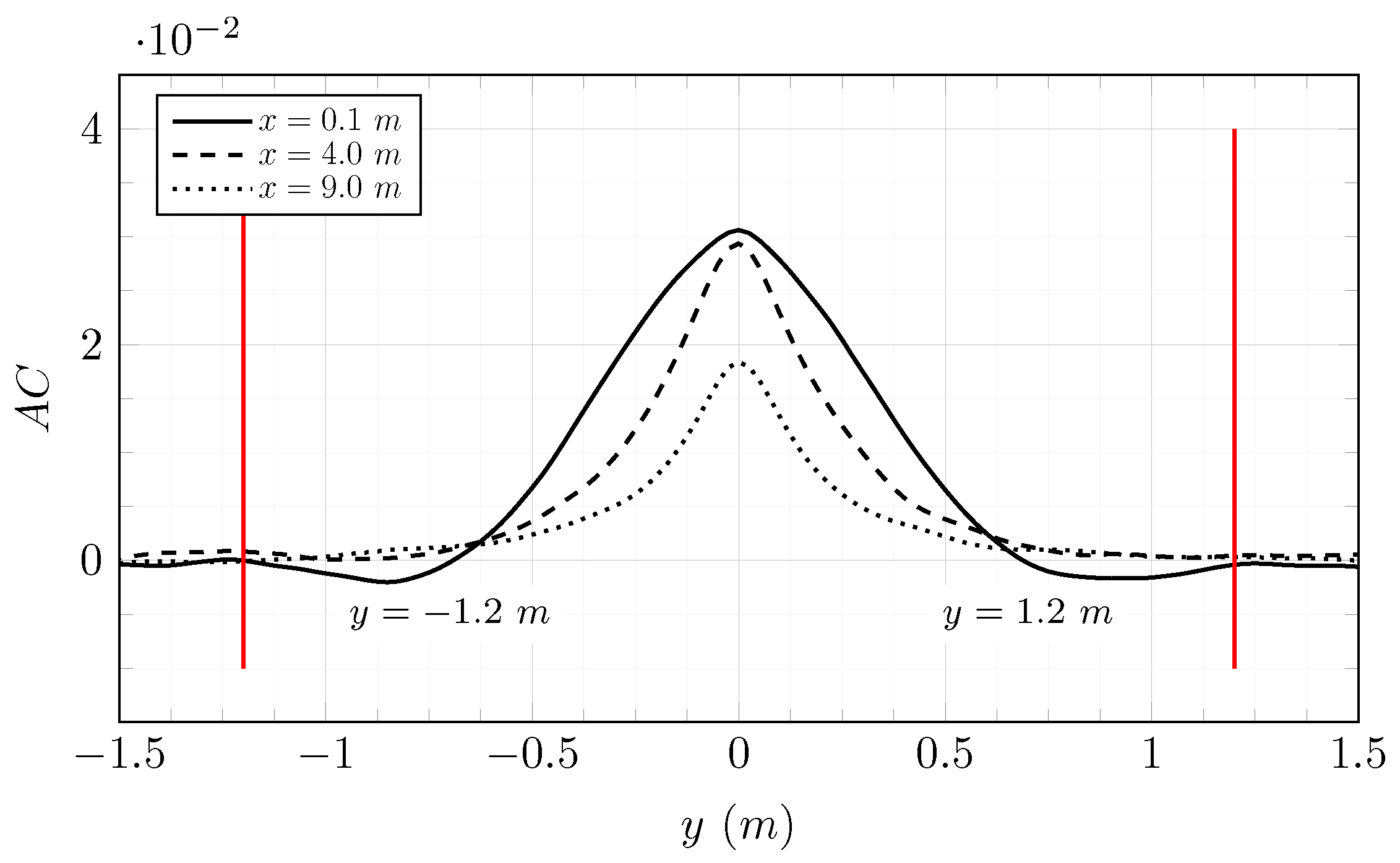
4.3. Spatial Analysis

Spatial analysis is based on instantaneous pressure maps of the wake. Those maps are in the $\mathit{xz}$ and $\mathit{xy}$ plans and contain the axis of rotation. There is 13 moments (26 maps) for the cases $I=\left[0,3\right]\%$ and 30 moments (60 maps) for the cases $I=\left[8,12.5\right]\%$. Intersections between plans and tip-vortices are identified with pressure minima. Locations of intersections are then recorded regardless of the moments or maps they are from. The sampling rate of the moments is 2 Hz.

The wake is divided according to the stream-wise direction into segments of $0.5$ m spaced $0.25$ m apart. The number of intersections per segment is $N_i$. If $x_0$ is the lower limit of a segment, the first segment is at $x_0=0.5$ m and the last at $x_0=2.5$ m. The number of intersections in the first segment is $N_0$ and the ratio $N_t=N_i/N_0$ is the intersections rate. It gives an estimation of the loss of consistency of tip-vortices. 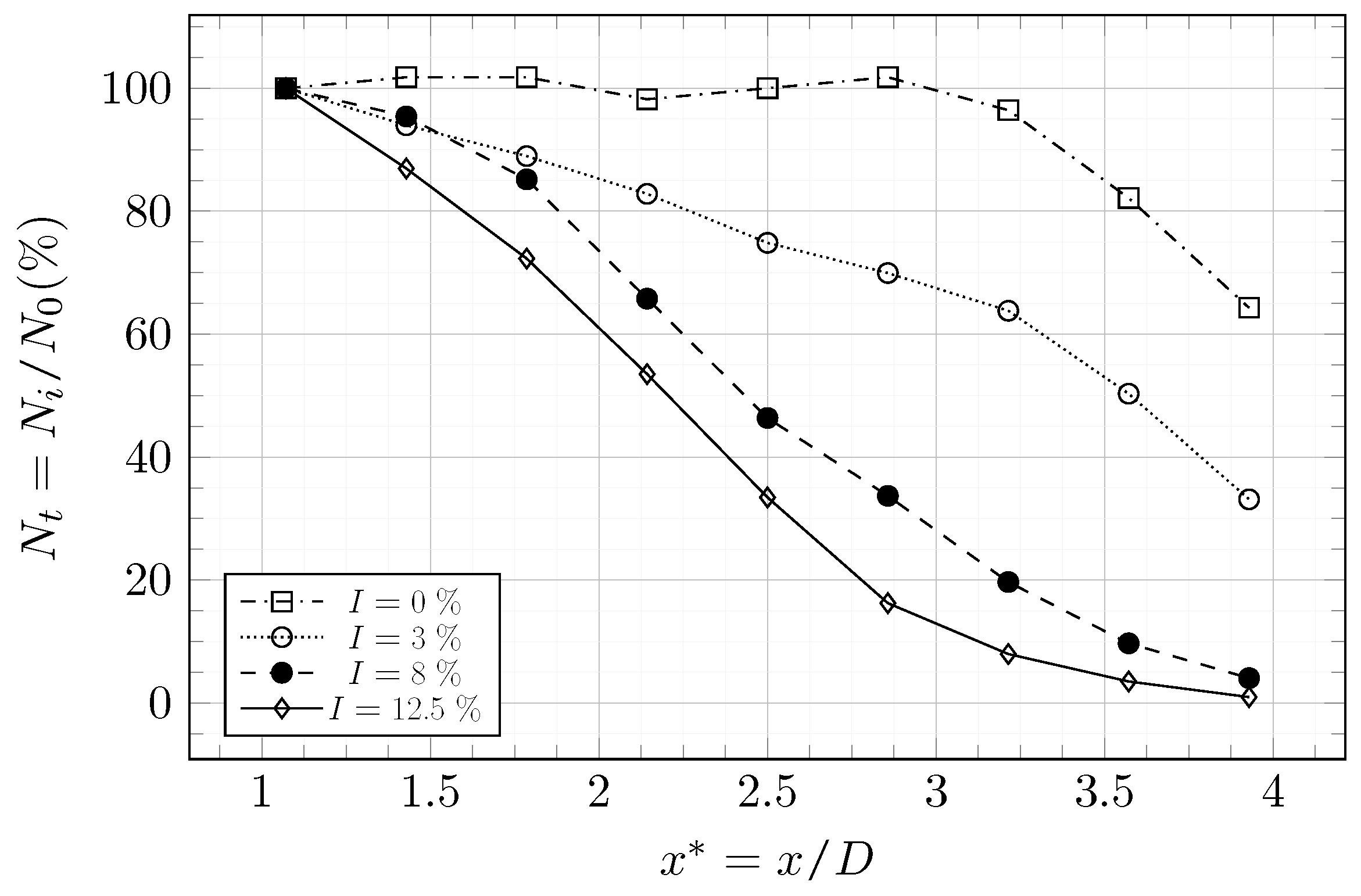Figure 27 shows the evolution of $N_t$ according to the stream-wise direction. Without upstream turbulence, the tip-vortices are still consistent after $x=3D$. It confirms what is observed in Figure 25a. Even a low turbulence intensity ($I=3\%$) has an influence over tip-vortices consistency. This was also observed in Figure 25b and in Figure 23. On that last one, the peak of turbulence intensity $I_{2D_{bis}}$ generated by tip-vortices is hardly observable at $x=3D$. With an upstream turbulence intensity of $I=\left[8,12.5\right]\%$, tip-vortices rapidly lose their consistency (Figure 25d). An analysis based on the height of tip-vortices is now carried out to have more detailed knowledge of the influence of turbulence over tip-vortices propagation.

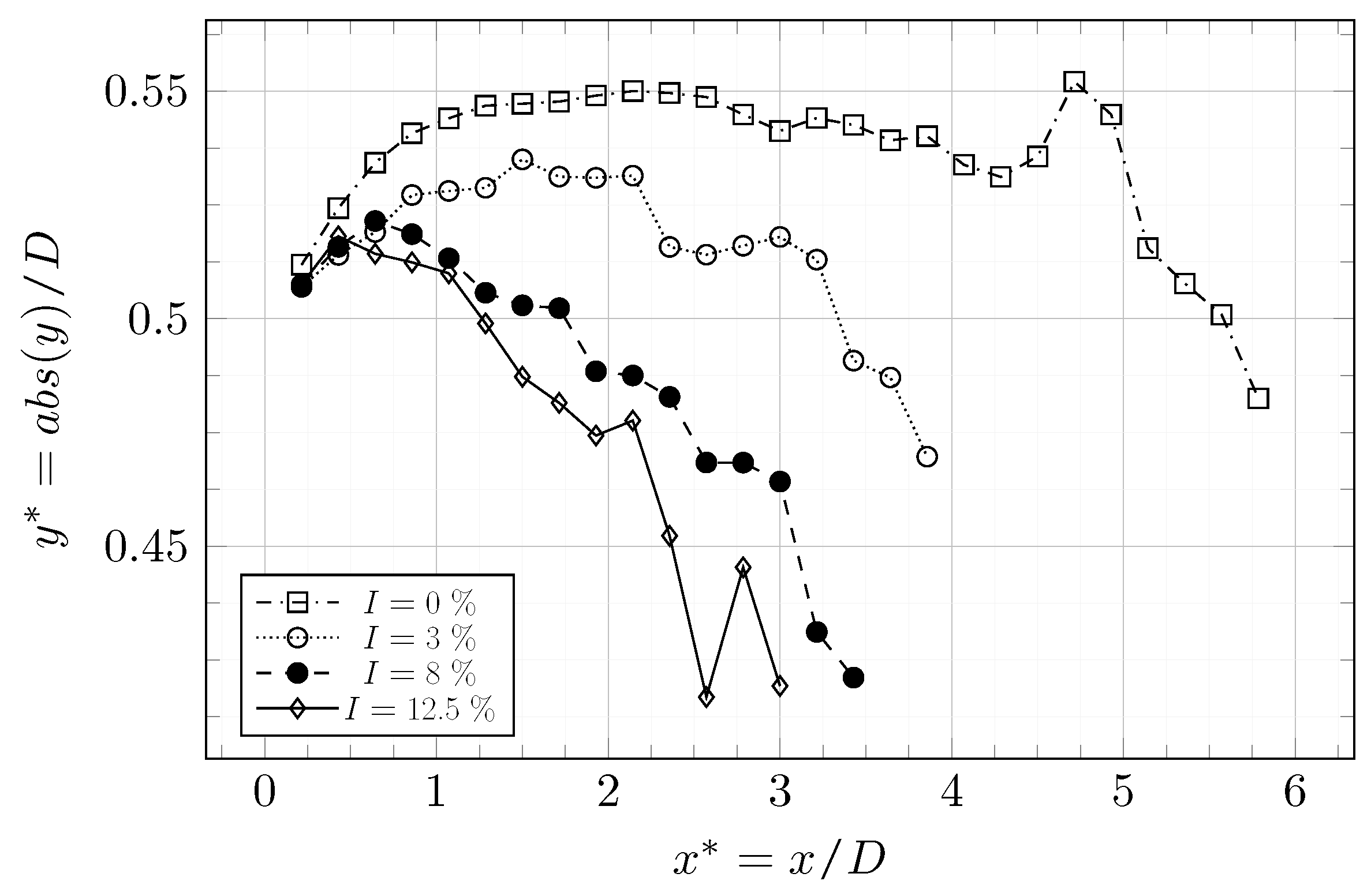
Figure 28 shows the distance $y^{*}$ from the intersections to the axis $y=z=0$ m. The height $y^{*}$ is averaged over $0.3$ m segments from $x_0=0$ m until $N_t<30\%$. The height $y^{*}$ decreases faster as the turbulence increases. A higher upstream turbulence intensity thus increases the trend of tip-vortices to move toward the axis $y=z=0$ m. The low turbulence rate $I=3\%$ as a significant impact over $y^{*}$ and the evolution of $y^{*}$ for the cases with $I=\left[8,12.5\right]$ are close.

An analysis of tip-vortices propagation has been carried out. Several trends that are consistent with observations made in the previous section have been highlighted. Since one of the main sources of turbulence in the close wake is tip-vortices, additional comments about the results of the previous section can be made. In Figure 20, a difference between the simulation and the experiment is observed at $x=1.2D$. The turbulence intensity from the simulation is too low compared to the experiment. By considering observations made on tip-vortices, a third source of error can be suggested. Tip-vortices may move too quickly toward the axis $y=z=0$ m, modifying the shape of turbulence intensity profiles. It is known that the integral length scale for the case $I=12.5\%$ is larger in the simulation than in the experiment. The integral length scale of the turbulence may influence the propagation of tip-vortices, and modify the turbulence intensity profiles.

5. Conclusions

1.

The modelling of a tidal turbine in a turbulence flow with an open-source LBM solver has been performed. To achieved this, an IBM boundary condition coupled to a wall model and a synthetic turbulence generation algorithm were implemented in the code.

2.

A realistic upstream turbulent condition has been validated for an LBM-LES tidal turbine modelling. For low turbulence rates, it has been observed that the choice of parameter is straightforward. The characteristics of the synthetic turbulence match experimental ones. It has been found that for a high turbulence rate, compromises have to be made in order to keep the turbulence rate high enough. As a consequence, the integral length scale of the synthetic turbulence is greater than the experimental one.

3.

Blade resolved IBM-LBM-LES simulations of a three-bladed HATT have been carried out for two turbulent rates. Three meshes have been tested to estimate the mesh sensitivity of the approach. It has been observed that the mesh convergence in the thrust coefficient is quickly reached. Differences in power coefficient are still observed for the finest mesh. For the high turbulence rate case, those differences may come from the upstream synthetic turbulence.

4.

Average wake quantities from LBM-LES simulations have been compared with experimental ones. It has been observed that refining the mesh has little influence over the average wake. It slightly improves the predicted average axial velocity in the close wake. Elsewhere in the wake, average quantities computed with the LBM-LES are in accordance with experimental data. The influence of turbulence on the turbine behaviour is well predicted by the model.

5.

A third case has been simulated with an upstream turbulence rate of $I=8\%$. A cross-comparison has been carried out between wakes of the three different cases $I=\left[3,8,12.5\right]\%$. The evolution of the averaged velocity deficit is quite intuitive. This is not the case for other quantities. Turbulence intensity and shear stress from cases $I=3\%$ and $I=8\%$ are close whereas for tip-vortices evolution, cases $I=8\%$ and $I=12.5\%$ are close. Based on turbulence intensity, shear stress and PSD, far wakes of the three cases converge toward similar states.

6.

It has been observed with iso-surfaces of ${\lambda }_2$ criterion that typical wake structures like tip-vortices are greatly influenced by ambient turbulence. An analysis of the evolution of tip-vortices in the wake has been proposed. The envelope of tip-vortices is shortened in the $\mathit{x}$ direction and shrunk toward the axis with the increase in turbulence rate. The close wake is thus greatly influenced by the upstream turbulence.

7.

Improvements to the model or further investigations can be suggested. Studying the influence of the integral length scale on the wake is an interesting lead. It would confirm or invalidate some of the hypotheses made. Finally, improvements of the boundary layer model are one of the top priorities. It would allow for proper force computation. If forces from the simulations are reliable enough, it is then possible to estimate the turbulence-induced fatigue. Such information is substantial for turbine optimization.