Optimal Power Systems Restoration Based on Energy Quality and Stability Criteria

Abstract

Electric power systems (EPS) are exposed to disconnections of their elements, such as transmission lines and generation units, due to meteorological factors or electrical failures. Thus, this research proposes a smart methodology for the re-entry of elements that have been disconnected from the EPS due to unforeseen events. This methodology is based on optimal AC power flows (OPF-AC) which allow verifying the state of variables such as voltage, angular deviation, and power (these variables are monitored in normal and fault conditions). The proposed study considers contingencies N-2, N-3, N-4, and N-5, for which the disconnection of transmission lines and generation units are carried out randomly. The analysis of the EPS after the disconnections of the elements is carried out by means of the contingency index, with which the impact that the disconnections of the elements have on the EPS is verified. In this way, the optimal route is generated to restore the elements that went out of operation, verifying that when the elements re-enter the acceptable limits, voltage and voltage angle are not exceeded. According to the results of the methodology used, it was found that NM contingencies can be applied in the proposed model, in addition to considering stability restrictions, modeled as restrictions on acceptable voltage limits, and a new restriction for the voltage angle between the differences of the bars.

1. Introduction

Nowadays, electrical power systems (EPS) are a fundamental part of the modern world since they are responsible for providing the electricity supply by supplying electricity for commercial, industrial, and residential users. The electrical systems are not exempt from failures; due to this, outages in the electrical service can be generated causing great economic losses. In addition, power outages affect a wide variety of institutions and departments, and among these, there are some considered of high importance: those that must have continuous electricity supply such as police, military and fire departments, hospitals, clinics, and health care centers. Therefore, it is of utmost importance that the restoration of the operation of the electrical power system is carried out in the shortest possible time, through maneuvers and corrective actions in a way that does not affect the continuity, quality, and stability of the electric power supply [1,2,3].

There are factors that affect the EPS which cause it to stop supplying the electricity, such as connection and disconnection of loads and generation units, meteorological phenomena such as lightning, and bad maneuvering of EPS operators. The presence of these events generates disturbances in the electrical system causing oscillations, overvoltages, and overcurrents; in addition, it causes elements such as transmission lines, generators, and loads to be out of operation. The disconnection of transmission lines, generators, and loads can cause loss of stability in EPS and a disconnection cascade effect in most elements, which would lead to a partial or total blackout of the EPS [2,3,4,5].

Reestablishing the energy at the EPS goes beyond reconnecting generation units and transmission elements. Therefore, decision-making methodologies must be planned and determined, in addition to establishing steps so that the electrical system restoration complies with the quality and stability indexes. For the reason previously explained, it is necessary to take into account the following guidelines: know how the electrical power system is operating under normal conditions and under post-failure conditions, carry out a planning that ensures that the electrical system recovers its normal operation in the shortest possible time, determine the way for reconnection of the elements of the generation system, and the route for the entrance to the system of power transformers and transmission lines. The planning and methodology that will be determined and used for the restoration of the EPS should allow reducing generation costs caused by the power outages, in addition, to reduce the time used in the necessary maneuvers to reconnect the elements that went out of operation by evaluating technical criteria for the re-establishment of the normal operation of the EPS [6,7,8].

Refs. [9,10] used the mixed integer linear programming (MILP) technique, which is used to determine the sequence in which the generators must enter. The authors also used the improved Dijkstra method, significantly reducing the time taken for the generators to start.

The authors of [6] used various techniques for the restoration of EPS, dividing the problem into several stages: (i) using the MILP optimization technique, determining the input order of the generators, and (ii) using decision theory heuristics. This methodology has an interesting characteristic since it does not need to use technical variables such as voltage and current obtained from the EPS and its main objective is to ensure the generators reach their maximum power. Finally, for the restoration of the transmission system, a genetic algorithm is used.

The use of the water cycle algorithm (WCA) as a methodology to restore EPS is proposed in [11], which takes into account various quality and reliability indexes to achieve the restoration of the EPS. This article considers the restoration of the transmission system. In addition, the results obtained from the WCA technique are compared with the particle swarm optimization heuristics (PSO) and the genetic algorithm (GA), where the water cycle algorithm methodology generates the optimal solution in less time than the PSO and the GA.

Contingency analysis allows studying the severity of elements disconnection in the power system; therefore, it is essential to consider its study. It is called contingency when one or more elements are disconnected from the electrical system unexpectedly due to unscheduled or unforeseen events such as wrong practices during maintenance of the electrical system. The operating outage of the following elements is considered a contingency: generators, loads, transmission lines, and transformers. To carry out the contingency analysis of the EPS, optimal power flows (OPF) are used to calculate variables such as current, voltage, frequency, and power. In this way, it is possible to know the post-contingency state of the EPS [12,13].

There are different methodologies that allow analyzing what happened in the EPS in the event of a failure or a contingency, for example, OPF-AC and optimal DC power flow (OPF-DC). Furthermore, in these types of problems, it is necessary to use OPF-AC and OPF-DC to determine the contingency indexes, which helps to determine which element of the EPS is most affected after a failure. These methodologies are used to determine generation dispatch cost and observe variables of voltage, angle, frequency, current, and technical losses through the power balance [14,15,16,17,18].

State estimators (SE) allow the EPS to be monitored and are widely used by control centers to determine the state of the electrical power system. SE are useful to observe how the network is operating and contribute when it is the time of restoring the EPS since they allow to know the operating status of the EPS under normal conditions and in the event of failures or contingencies. The SE consist of sensors and meters placed throughout the electrical system, allowing it to process and interpret the operating variables of the EPS in real-time [19,20]. In [21], a state estimator is presented which has as an objective to verify the post-contingency state when disconnecting a transmission line by generating contingencies N-1; this is performed through the transmission line outage post-contingency state estimator principle (PLOP).

In [22], the authors propose a method to determine the state of the EPS after suffering the disconnection of transmission lines. The model is based on data obtained by the phasor measurement units (PMU) in pre-failure and post-failure when applying statistical procedures. To implement this methodology it is necessary to linearize the power flow of the EPS.

In [23], the authors present a particular data concentrator, this concentrator is a data acquisition suspension clamp that can be used in electrical conductors, for transmission lines, communication lines, water lines, gas lines, and oil lines. This type of clamp allows to monitor, acquire, and generate reports of different EPS elements. The main disadvantage of the measuring mechanism is that its use as part of a clamp is restricted.

In [24], the authors propose the use of sensors to monitor the electrical parameters on both sides of a switching device; in this way, they observe the number of power outages that occurred in the EPS, in addition to the duration and the voltage deviation that causes the suspension of power supply. These sensors are installed in the outgoing electrical transmission lines and in the low-voltage busbars of the transformer substation.

In [25], the authors propose the use of networks of power lines sensors; the sensors allow to monitor the variables in real time, and they also evaluate variables such as the thermal capacity of the transmission lines, contacts of overhead conductors with vegetation, and proximity between overhead power lines and animals in real time.

EPS stability is the system’s ability to bring back its operation to steady-state condition when suffering electrical failures or disturbances that destabilize the electrical system.If the electrical system becomes unstable, it generates significant variations in the voltage, angle and frequency parameters, causing the disconnection of transmission lines and generation units, in addition to possible total or partial blackouts. There are three parameters that are fundamental for the study of EPS stability, such as angle, frequency, and voltage, which are related to each other [26,27], so when reconnecting, it is important that the EPS meets these requirements. Only in this way can the elements that suffered a disconnection be entered.

In this research, a methodology is proposed that allows the restoration of the electrical system considering optimal operating costs. For this purpose, a review of the state of the art regarding the problem posed was established in the previous section to obtain the proposed scenario for this work. To solve the problem, two methodologies were used: the contingency index and the OPF-AC; which were applied to the normal operating state of the EPS and to contingencies generated randomly. It should be emphasized that the scenario in which the EPS suffers a black-start is not taken into consideration; this scenario will be carried out in future works. Through the contingency index, a decision tree was generated, which allowed establishing the path or route to reconnect the elements to the electrical system. The architecture of this article is shown in Figure 1.

2. Electrical Power System Operation

2.1. Electrical Power System Restoration

Electrical power system reestablishment is a process that demands more than planning and analysis of the electrical system variable. First, a verification of the available elements must be carried out, as well as decision-making tools for the EPS operators. Restoring the EPS is a multi-objective optimization problem with variables and constraints that are nonlinear character [28]. The restoration objective is for the system to return to normal operating conditions quickly and safely, minimizing the time it takes to recover normal operating conditions and preventing instability in the EPS due to elements reconnection that went out of operation. These actions will reduce the partial or total EPS outage [29]. The steps for EPS restoration are detailed below.

• Preparing the EPS for restoration: The first step consists of checking the status of the EPS after one or more contingencies have occurred, in addition to verifying the limits of the technical variables such as voltage, current, frequency, and angular deviation. The EPS capacity must be verified in terms of elements that are available to enter and provide electrical power to the EPS. Additionally, due to their intermittency nature, renewable generation should be taken out of service [7].
• Strategies for EPS restoration: There are two specific strategies used in the EPS restoration, (i) reduction and (ii) accumulation. The first consists of re-entering transmission lines and generation, and, as the last priority, the loads. By doing this, it is intended to stabilize the electrical system with the reestablishment of the transmission part of the electrical power system. The accumulation method consists of two steps: first, the transmission system with its more significant loads is reconnected to the electrical power system, and then, as a second step, the remaining (noncritical) loads are reconnected [7].
• Subsystems characterization of the electrical power system: When electrical failures occur in the EPS, causing contingencies, for the restoration of the system it is necessary to consider the accumulation strategy because it is the most used to solve these types of problems. Therefore, it must be taken into account that to work under this method, it is necessary to divide the system into several subsystems, fulfilling characteristics such as having a reduced difference margin between generation and loads in each subsystem, and the subsystems must be balanced. Reactive power must be checked in a special way, since it is one of the main factors in restoring the EPS [7].
• Re-entry of the transmission system: Reconnecting the transmission system is a complicated process; it is necessary to comply with the minimum and maximum voltage limits, verifying that the system does not violate any of these. Energization is achieved by two methods: line switching and load currents.
• Energization for load and generation: The energization of the generation system is the most complicated step, because this action must be carried out in the shortest possible time in order not to stop supplying electrical energy to critical loads such as hospitals, police stations, firefighters, and military services. When the generators enter the system, the stability of the EPS is also verified by checking the voltage and frequency for the input of the loads, and it must be verified that the generation capacity is proportional to the load capacity that is entering the system.
• System synchronization: Having most of the EPS restored, it must be verified that the system is synchronized by checking the magnitudes of voltages, voltage sequence, and frequency. The transmission system must also comply with adequate synchronization; for this, the system must be evaluated by means of the power quality indexes, in addition to checking the capacity of the transmission lines.

There are several characteristics for the restoration of the EPS; in [30], several are mentioned, such as:

• Voltage and frequency control.
• Active power distribution in weak subsystems.
• Capacity that the electrical system must have to start in initial conditions through thermal power plants.
• Reactive power capacity for connecting transformers and transmission lines.

Optimal power flows (OPF) are key methods to solve restoration power problems. In addition, it is necessary to use several techniques for the restoration of the EPS; among them, there are contingency and quality indexes. The post-failure stability of the system should be considered once the elements that were affected by contingencies re-enter the system.

Optimal power flows (OPF) are used to solve problems where there are a large number of variables, high uncertainty, and the system is robust; they are specially used to solve stochastic optimization problems [31,32,33].

The AC-OPF method allows solving resilience problems because it involves a large number of technical variables of the EPS. In addition, OPF-AC is the most effective method in solving these types of electrical system restoration problems. The fundamental objective of OPF-AC is to minimize generation operating costs, taking into account operating restrictions of the system, for example, voltage limits, angular deviation, and power balances [34].

The equations that intervene in the calculation of the OPF-AC are given as follows:

• Objective Function

  $$MinZ=\sum _{i=1}^n{C}_{gi}$$

  (1)
• Restrictions

  $$P_{gi}-P_{Di}=V_i\sum _{j=1}^n{V}_j{Y}_{ij}Cos({\delta }_i-{\delta }_j-{\theta }_{ij})$$

  (2)

  $$Q_{gi}-Q_{Di}=V_i\sum _{j=1}^n{V}_j{Y}_{ij}Sin({\delta }_i-{\delta }_j-{\theta }_{ij})$$

  (3)

  $$P_g^{min}\le P_g\le P_g^{max}$$

  (4)

  $$Q_g^{min}\le Q_g\le Q_g^{max}$$

  (5)

  $$V_i^{min}\le V_i\le V_i^{max}$$

  (6)

  $${\delta }_i^{min}\le {\delta }_i\le {\delta }_i^{max}$$

  (7)

Equation (1) represents the objective function, which consists of minimizing the operating cost in generation, while Equations (2) and (3) represent the active and reactive power balance restrictions for the EPS. Equations (4) and (5) represent the limits of active power and reactive power. Finally, Equations (6) and (7) represent the operating limits of voltage and angular deviation of the system.

2.2. Quality and Stability for the Restoration of the EPS

Voltage stability in the EPS is determined by the ability to recover the voltage in all the bus bars after suffering electrical faults or disturbances directly affecting the normal operation of the system. The active or reactive power imbalance that may exist between demand and generation is the main cause of voltage instability. This causes the voltage to rise drastically, exceeding the admissible limits, resulting in the system protections acting; thus, elements of the EPS move out in a cascading effect. If the voltage fluctuations occur abruptly, it is due to an oscillation in the rotor angle of the synchronous machine [26].

Angle stability is directly related to a synchronous machine’s ability to withstand a disturbance and continue to operate; consequently, there must be a condition in which the electromagnetic and mechanical torque must be balanced, that is, they must be equal. If this condition is not met, angular oscillations occur, causing the output of one or more generators from the electrical system. When small disturbances occur, synchronous generators suffer oscillations in the rotor; however, when these events occur, the generation units have the ability to solve the problem of small disturbances and continue operating. On the contrary, if large-scale disturbances occur, the angular stability of the synchronous machine is lost, which causes the operating output of the said unit [35,36].

To prevent the system from losing stability in the face of events that generate contingencies in [37], it is suggested that this parameter is bordering $\pm 35$ degrees or $\pm 0.6$ radians, this means that when disconnections of elements occur, the angle does not exceed 90 degrees, this being the limit of stability in steady state. If the angle exceeds 90 degrees, the system would go into instability.

The energy quality of the electrical power systems worldwide is generally regulated by each country and the established limits are $\pm 5\%$ and $\pm 10\%$; however, for the resolution of the problem of resilience in [38], it is mentioned that the quality limits are 1.05 pu and 0.95 pu, that is, the $\pm 5\%$, this value is taken to avoid a system collapse when generating N-M contingencies.

2.3. Contingency Index

The contingency index (CI) is used to determine the state of the electrical system under normal conditions and when contingencies are generated. If the EPS is in a normal state, considering that lines and generators are within the operating limits, the CI value will be low; on the contrary, if there are external events that lead to the disconnection of EPS elements, the CI will increase accordingly to the severity of the disconnect. The CI is ordered from highest to lowest, then we proceed to verify that the initial cases are the most damaging, causing violations of capacity limits and nodal voltage limits.

Equation (8) shows how to calculate the contingency index, the weighting factor $W_{fi}$ indicates the importance of the transmission lines for the system, and the values that are normally assigned depend on transmission lines chargeability. In this research, the value for the weighting factor is one, giving the same importance to all the elements. The factor n, known as the evaluation factor, helps to reduce the error when ordering the contingencies and fulfills a restriction $n\ge 1$. The factor $f_i$ represents the power flow in the lines of the EPS or voltages in the nodes of the system; therefore, it has two different contingency indexes and must be studied as such [39,40,41].

$$CI=\sum _{l=1}^{nl}\left(\frac{W_{fi}}{2n}\right){\left(\frac{f_i}{f_i^{max}}\right)}^{2n}$$

(8)

3. Problem Formulation

As the EPS is exposed to electrical failures or events that generate contingencies, it is necessary to plan and develop a methodology that allows the system to be optimally restored; therefore, the OPF-AC study has been carried out, generating a generic algorithm that allows determining the technical variables of (i) voltage, (ii) angular deviation, and (iii) power flow. In addition, N-2, N-3, N-4, and N-5 contingencies are considered, and through the continence index, a decision tree was developed, which allows appreciating the route that must be followed to optimally restore the EPS.

Four cases were studied, generating contingencies N-2, N-3, N-4, and N-5, with case A being the disconnection of a line and a generator, case B disconnection of two transmission lines, case C exit from the operation of two generators, case D the disconnection of two lines and a generator, case E the disconnection of three lines and a generator, and case F the disconnection of four transmission lines and a generator. In each of the case studies, in addition to contingencies, the normal behavior of the electrical system is analyzed. The disconnection of transmission lines and generators was carried out randomly, without considering the collection of the lines or the contribution of the generators that went out of operation. The study was conducted on the generic IEEE 118 bus system which is presented in Figure 2.

Table A1. IEEE 118 bar system generation data.

Name	Bus No.	Pmin	Pmax	Qmin	Qmax
TG1	4	5	30	−300	300
TG2	6	5	30	−13	50
TG3	8	5	30	−300	300
TG4	10	150	500	−147	200
TG5	12	100	300	−35	120
TG6	15	10	30	−10	30
TG7	18	25	100	−16	50
TG8	19	5	30	−8	24
TG9	24	5	30	−300	300
TG10	25	100	300	−47	140
TG11	26	100	350	−1000	1000
TG12	27	8	30	−300	300
TG13	31	8	30	−300	300
TG14	32	25	100	−14	42
TG15	34	8	30	−8	24
TG16	36	25	100	−8	24
TG17	40	8	30	−300	300
TG18	42	8	30	−300	300
TG19	46	25	100	−100	100
TG20	49	50	250	−85	210
TG21	54	50	250	−300	300
TG22	55	25	100	−8	23
TG23	56	25	100	−8	15
TG24	59	50	200	−60	180
TG25	61	50	200	−100	300
TG26	62	25	100	−20	20
TG27	65	100	420	−67	200
TG28	66	100	420	−67	200
TG29	69	80	300	−99,999	99,999
TG30	70	30	80	−10	32
TG31	72	10	30	−100	100
TG32	73	5	30	−100	100
TG33	74	5	20	−6	9
TG34	76	25	100	−8	23
TG35	77	25	100	−20	70
TG36	80	150	500	−165	280
TG37	82	25	100	−9900	9900
TG38	85	10	30	−8	23
TG39	87	200	650	−100	1000
TG40	89	150	500	−210	300
TG41	90	8	20	−300	300
TG42	91	20	50	−100	100
TG43	92	100	300	−3	9
TG44	99	100	300	−100	100
TG45	100	100	300	−50	155
TG46	103	8	20	−15	40
TG47	104	25	100	−8	23
TG48	105	25	100	−8	23
TG49	107	8	20	−200	200
TG50	110	25	50	−8	23
TG51	111	25	100	−100	1000
TG52	112	25	100	−100	1000
TG53	113	25	100	−100	200
TG54	116	25	50	−1000	1000

represents the input data of the generators,

Table A2. IEEE 118 bar system bus data.

Index	R	X	B	Index	R	X	B
1	0.0303	0.0999	0.0254	94	0.00172	0.02	0.216
2	0.0129	0.0424	0.01082	95	0	0.0268	0
3	0.00176	0.00798	0.0021	96	0.00901	0.0986	1.046
4	0.0241	0.108	0.0284	97	0.00269	0.0302	0.38
5	0.0119	0.054	0.01426	98	0.018	0.0919	0.0248
6	0.00459	0.0208	0.0055	99	0.018	0.0919	0.0248
7	0.00244	0.0305	1.162	100	0.0482	0.218	0.0578
8	0	0.0267	0	101	0.0258	0.117	0.031
9	0.00258	0.0322	1.23	102	0	0.037	0
10	0.0209	0.0688	0.01748	103	0.0224	0.1015	0.02682
11	0.0203	0.0682	0.01738	104	0.00138	0.016	0.638
12	0.00595	0.0196	0.00502	105	0.0844	0.2778	0.07092
13	0.0187	0.0616	0.01572	106	0.0985	0.324	0.0828
14	0.0484	0.16	0.0406	107	0	0.037	0
15	0.00862	0.034	0.00874	108	0.03	0.127	0.122
16	0.02225	0.0731	0.01876	109	0.00221	0.4115	0.10198
17	0.0215	0.0707	0.01816	110	0.00882	0.0355	0.00878
18	0.0744	0.2444	0.06268	111	0.0488	0.196	0.0488
19	0.0595	0.195	0.0502	112	0.0446	0.18	0.04444
20	0.0212	0.0834	0.0214	113	0.00866	0.0454	0.01178
21	0.0132	0.0437	0.0444	114	0.0401	0.1323	0.03368
22	0.0454	0.1801	0.0466	115	0.0428	0.141	0.036
23	0.0123	0.0505	0.01298	116	0.0405	0.122	0.124
24	0.01119	0.0493	0.01142	117	0.0123	0.0406	0.01034
25	0.0252	0.117	0.0298	118	0.0444	0.148	0.0368
26	0.012	0.0394	0.0101	119	0.0309	0.101	0.1038
27	0.0183	0.0849	0.0216	120	0.0601	0.1999	0.04978
28	0.0209	0.097	0.0246	121	0.00376	0.0124	0.01264
29	0.0342	0.159	0.0404	122	0.00546	0.0244	0.00648
30	0.0135	0.0492	0.0498	123	0.017	0.0485	0.0472
31	0.0156	0.08	0.0864	124	0.0294	0.105	0.0228
32	0	0.0382	0	125	0.0156	0.0704	0.0187
33	0.0318	0.163	0.1764	126	0.00175	0.0202	0.808
34	0.01913	0.0855	0.0216	127	0	0.037	0
35	0.0237	0.0943	0.0238	128	0.0298	0.0853	0.08174
36	0	0.0388	0	129	0.0112	0.03665	0.03796
37	0.00431	0.0504	0.514	130	0.0625	0.132	0.0258
38	0.00799	0.086	0.908	131	0.043	0.148	0.0348
39	0.0474	0.1563	0.0399	132	0.0302	0.0641	0.01234
40	0.0108	0.0331	0.0083	133	0.035	0.123	0.0276
41	0.0317	0.1153	0.1173	134	0.02828	0.2074	0.0445
42	0.0298	0.0985	0.0251	135	0.02	0.102	0.0276
43	0.0229	0.0755	0.01926	136	0.0239	0.173	0.047
44	0.038	0.1244	0.03194	137	0.0139	0.0712	0.01934
45	0.0752	0.247	0.0632	138	0.0518	0.188	0.0528
46	0.00224	0.0102	0.00268	139	0.0238	0.0997	0.106
47	0.011	0.0497	0.01318	140	0.0254	0.0836	0.0214
48	0.0415	0.142	0.0366	141	0.0099	0.0505	0.0548
49	0.00871	0.0268	0.00568	142	0.0393	0.1581	0.0414
50	0.00256	0.0094	0.00984	143	0.0387	0.1272	0.03268
51	0	0.0375	0	144	0.0258	0.0848	0.0218
52	0.0321	0.106	0.027	145	0.0481	0.158	0.0406
53	0.0593	0.168	0.042	146	0.0223	0.0732	0.01876
54	0.00464	0.054	0.422	147	0.0132	0.0434	0.0111
55	0.0184	0.0605	0.01552	148	0.0356	0.182	0.0494
56	0.0145	0.0487	0.01222	149	0.0162	0.053	0.0544
57	0.0555	0.183	0.0466	150	0.0269	0.0869	0.023
58	0.041	0.135	0.0344	151	0.0183	0.0934	0.0254
59	0.0608	0.2454	0.06068	152	0.0238	0.108	0.0286
60	0.0413	0.1681	0.04226	153	0.0454	0.206	0.0546
61	0.0224	0.0901	0.0224	154	0.0648	0.295	0.0472
62	0.04	0.1356	0.0332	155	0.0178	0.058	0.0604
63	0.038	0.127	0.0316	156	0.0171	0.0547	0.01474
64	0.0601	0.189	0.0472	157	0.0173	0.0885	0.024
65	0.0191	0.0625	0.01604	158	0.0397	0.179	0.0476
66	0.0715	0.323	0.086	159	0.018	0.0813	0.0216
67	0.0715	0.323	0.086	160	0.0277	0.1262	0.0328
68	0.0684	0.186	0.0444	161	0.0123	0.0559	0.01464
69	0.0179	0.0505	0.01258	162	0.0246	0.112	0.0294
70	0.0267	0.0752	0.01874	163	0.016	0.0525	0.0536
71	0.0486	0.137	0.0342	164	0.0451	0.204	0.0541
72	0.0203	0.0588	0.01396	165	0.0466	0.1584	0.0407
73	0.0405	0.1635	0.04058	166	0.0535	0.1625	0.0408
74	0.0263	0.122	0.031	167	0.0605	0.229	0.062
75	0.073	0.289	0.0738	168	0.00994	0.0378	0.00986
76	0.0869	0.291	0.073	169	0.014	0.0547	0.01434
77	0.0169	0.0707	0.0202	170	0.053	0.183	0.0472
78	0.00275	0.00955	0.00732	171	0.0261	0.0703	0.01844
79	0.00488	0.0151	0.00374	172	0.053	0.183	0.0472
80	0.0343	0.0966	0.0242	173	0.0105	0.0288	0.0076
81	0.0474	0.134	0.0332	174	0.03906	0.1813	0.0461
82	0.0343	0.0966	0.0242	175	0.0278	0.0762	0.0202
83	0.0255	0.0719	0.01788	176	0.022	0.0755	0.02
84	0.0503	0.2293	0.0598	177	0.0247	0.064	0.062
85	0.0825	0.251	0.0569	178	0.00913	0.0301	0.00768
86	0.0803	0.239	0.0536	179	0.0615	0.203	0.0518
87	0.04739	0.2158	0.05646	180	0.0135	0.0612	0.01628
88	0.0317	0.145	0.0376	181	0.0164	0.0741	0.01972
89	0.0328	0.15	0.0388	182	0.0023	0.0104	0.00276
90	0.00264	0.0135	0.01456	183	0.00034	0.00405	0.164
91	0.0123	0.0561	0.01468	184	0.0329	0.14	0.0358
92	0.00824	0.0376	0.0098	185	0.0145	0.0481	0.01198
93	0	0.0386	0	186	0.0164	0.0544	0.01356

represents the input data of the transmission lines, and, finally, we have the data of the loads that is given by

Table A3. IEEE 118 bar system load data.

Index	Name	BusNo	PL	QL	Index	Name	BusNo	PL	QL
1	Load1	1	54.14	28.66	46	Load46	56	84	18
2	Load2	2	21.23	955	47	Load47	57	12	3
3	Load3	3	41.4	10.62	48	Load48	58	12	3
4	Load4	4	31.85	12.74	49	Load49	59	277	113
5	Load5	6	55.2	23.35	50	Load50	60	78	3
6	Load6	7	20.17	2.12	51	Load51	62	77	14
7	Load7	11	74.31	24.42	52	Load52	66	39	18
8	Load8	12	49.89	10.62	53	Load53	67	28	7
9	Load9	13	36.09	16.99	54	Load54	70	66	20
10	Load10	14	14.86	1.06	55	Load55	74	68	27
11	Load11	15	95.54	31.85	56	Load56	75	47	11
12	Load12	16	26.54	10.62	57	Load57	76	68	36
13	Load13	17	11.68	3.18	58	Load58	77	61	28
14	Load14	18	63.69	36.09	59	Load59	78	71	26
15	Load15	19	47.77	26.54	60	Load60	79	39	32
16	Load16	20	19.11	3.18	61	Load61	80	130	26
17	Load17	21	14.86	8.49	62	Load62	82	54	27
18	Load18	22	10.62	5.31	63	Load63	83	20	10
19	Load19	23	7.43	3.18	64	Load64	84	11	7
20	Load20	27	65.82	13.8	65	Load65	85	24	15
21	Load21	28	18.05	7.43	66	Load66	86	21	10
22	Load22	29	25.48	4.25	67	Load67	88	48	10
23	Load23	31	45.65	28.66	68	Load68	90	78	42
24	Load24	32	62.63	24.42	69	Load69	92	65	10
25	Load25	33	24.42	9.55	70	Load70	93	12	7
26	Load26	34	62.63	27.6	71	Load71	94	30	16
27	Load27	35	35.03	9.55	72	Load72	95	42	31
28	Load28	36	32.91	18.05	73	Load73	96	38	15
29	Load29	39	27	11	74	Load74	97	15	9
30	Load30	40	20	23	75	Load75	98	34	8
31	Load31	41	37	10	76	Load76	100	37	18
32	Load32	42	37	23	77	Load77	101	22	15
33	Load33	43	18	7	78	Load78	102	5	3
34	Load34	44	16	8	79	Load79	103	23	16
35	Load35	45	53	22	80	Load80	104	38	25
36	Load36	46	28	10	81	Load81	105	31	26
37	Load37	47	34	0	82	Load82	106	43	16
38	Load38	48	20	11	83	Load83	107	28	12
39	Load39	49	87	30	84	Load84	108	2	1
40	Load40	50	17	4	85	Load85	109	8	3
41	Load41	51	17	8	86	Load86	110	39	30
42	Load42	52	18	5	87	Load87	112	25	13
43	Load43	53	23	11	88	Load88	114	8.49	3.18
44	Load44	54	113	32	89	Load89	115	23.35	7.43
45	Load45	55	63	22	90	Load90	117	21.23	8.49
					91	Load91	118	33	15

.   

Although the proposed method requires several input data, there are methods such as in [22,23,24,25], where they use elements such as sensors and data acquisition clamps that can monitor the EPS, thus providing the input data required from the proposed model.

Methodology

In the following, the methodology used to solve the problem of optimal restoration is detailed, by means of the pseudocode found in Algorithm 1. In Algorithm 1 it can be seen the steps to follow, such as entering the technical data of lines, generators and loads, applying the OPF-AC, generation of contingencies, the study of pre-failure and post-failure stability, and the development of the decision tree. It is important to emphasize that the implemented methodology is generic and, as such, it can be applied in any EPS, although input data is necessary to solve the problem.

Algorithm 1: Heuristics for optimal power systems restoration.

Step: 1 Input data EPS parameterization Lines: r, x, b Generator: $Pmin$, $Pmax$, $cost$, $Qmax$, $Qmin$, $Vg$ Load: $Pd$, $Pq$ Step: 2 OPF-AC O.F.:  $MinZ={\sum }_{i=1}^n{C}_{gi}$ s.t.: Power balance  $P_{giN-M}-P_{Di}=V_i{\sum }_{j=1}^n{V}_j{Y}_{ij}Cos({\delta }_i-{\delta }_j-{\theta }_{ij})$  $Q_{gi}-Q_{Di}=V_i{\sum }_{j=1}^n{V}_j{Y}_{ij}Sin({\delta }_i-{\delta }_j-{\theta }_{ij})$ Voltage and angle limits  $V_i^{min}\le V_i\le V_i^{max}$  $-\pi \le {\delta }_i\le \pi$ Save results:  $P_{ij},Q_{ij},V_i,{\delta }_i$ Step: 3 OPF-AC for contingencies generated Disconnection of one or more elements of the EPS $N-1$→ line or generator $N-2$→ line-line or generator-generator or line-generator $N-3$→   generator-line-line Calculated the OPF-AC for each case and contingency index for $i=1:n;n\in nodes$     for $j=1:n$         if $C_{ij}=1$                 $C_{ij}=0$                  $OPF-AC$                 $CI={\sum }_{l=1}^{nl}\left(\frac{W_{fi}}{2n}\right){\left(\frac{f_i}{f_i^{max}}\right)}^{2n}$                 $C_{ij}=1$                 $k=k+1$           end if      end for end for Step: 4 Decision tree for $k=1:m;m\in Contingencies$      if $C{I}_{ori}<C{I}_k$            Reestablishment of elements generating a path according to the CI            $C{I}_{ori}=C{I}_k$      end if end for Step: 5 Show results

Through Equation (8), the contingency index can be calculated. For this research, the voltage values in the system bus bars were used; in this way, the affectation suffered by the EPS when disconnecting one or more elements is quantified. The higher the value of the CI, the EPS suffers a greater affectation; according to this, the optimal restoration of the elements that previously went out of operation is planned. The elements that re-enter first are those that have the least impact on the EPS.

Below, there is a comparison of the existing models with the proposed method:

• In [4], the authors propose to restore the EPS by sectionalizing the system, taking into account the topology of the subsystems, and a restoration path is proposed. Therefore, all the elements that exist from the generation to the element in failure must be verified, something important in the methodology applied by the authors is that they will grant critical and noncritical loads, which are considered at the time of restoring the EPS; this would be a major disadvantage when performing a power system restoration.
• The authors in [6] propose the gap theory methodology for the restoration of the generation system in the EPS; this methodology implies the coordinated action of generation and load for the entry in sequence of the generating units. One of the advantages seen in this methodology is that there is great uncertainty in the data; the IGDT methodology is also called double uncertainty, while a great disadvantage is that, for the restoration of the system, the entry and exit of loads in the EPS are necessary.
• In [7], the authors propose to sectionalize the ESP to carry out the restoration of the generation system. They consider the capacity of the generators that did not go out of operation and the severity of those that went out of operation is determined, the restoration does not take into account the transmission system.
• In [9], the authors propose the restoration of the generation system by implementing a sequence for the start of the generators, taking into consideration the technical characteristics of the generators. One of the weaknesses of this method is that it is necessary to have a large amount of generation, otherwise the time of restoration of generators increases greatly.
• The methodology proposed in [10] considers the capacitance of the transmission lines; in addition, the method takes into account the path of the elements for restoration. The transmission lines enter interpretation and the importance is suggested according to the capacitance.
• In [11], the authors propose a methodology that consists of three steps after the sectioning of the EPS into subsystems. The first is to verify the generation units, the second is to reconfigure the subsystems, and the last step is to verify the problems that exist when reconfiguring the subsystems. Routes are carried out throughout the system and it is verified which is the option in which the best results are obtained.
• The proposed methodology is based on the reestablishment of the EPS, both in the generation and transmission systems in the presence of N-M contingencies. Stability criteria are taken, such as the voltage angle between the difference of the bars, as well as restrictions, such as the acceptable voltage limits, and the contingency index allows establishing the path for restoration. The proposed method does not consider the disconnection of loads nor the sectioning in EPS subsystems.
  Figure 3 represents the solution of the methodology used to solve the problem of optimal EPS restoration. As a first step, the EPS is selected and parameterized, followed by the OPF-AC, establishing the objective function and the restrictions. The contingencies are generated by disconnecting transmission lines and generating units. As a next step, the OPF-AC is carried out for each one of the contingencies generated; once the OPF-AC has been calculated for the contingencies, the CI is calculated, and the decision tree is made according to the calculated CI.

4. Analysis of Results

Once the proposed method mentioned in Section 3 has been executed, the results obtained in terms of voltage variations, angular deviation, and power flow in the bus bars of the study case in normal operational state and under contingencies are presented.

Finally, once the power flow has been performed in the EPS, the CI is determined using the power flow in the transmission lines, and the events that produce more damage to the electrical system were determined; that is, the CI is considered with the highest value. In this way, we proceed with the path for restoration, first entering the elements with the highest value of CI, then the elements of lower value of CI. The simulation was carried out using an interface between Gams 27.3 and Matlab R2021b, the algorithm was implemented in Matlab, which is in charge of processing the input data, and the results were returned by Gams after the optimization was completed. In this way, the OPF-AC is solved through nonlinear programming, using the CONOPT solver, in addition to calculating the CI.

The simulations implemented under the different software were run on a computer with an Intel Core I7 processor, 12 gigabyte RAM, Windows 10, and 64-bit operating system.

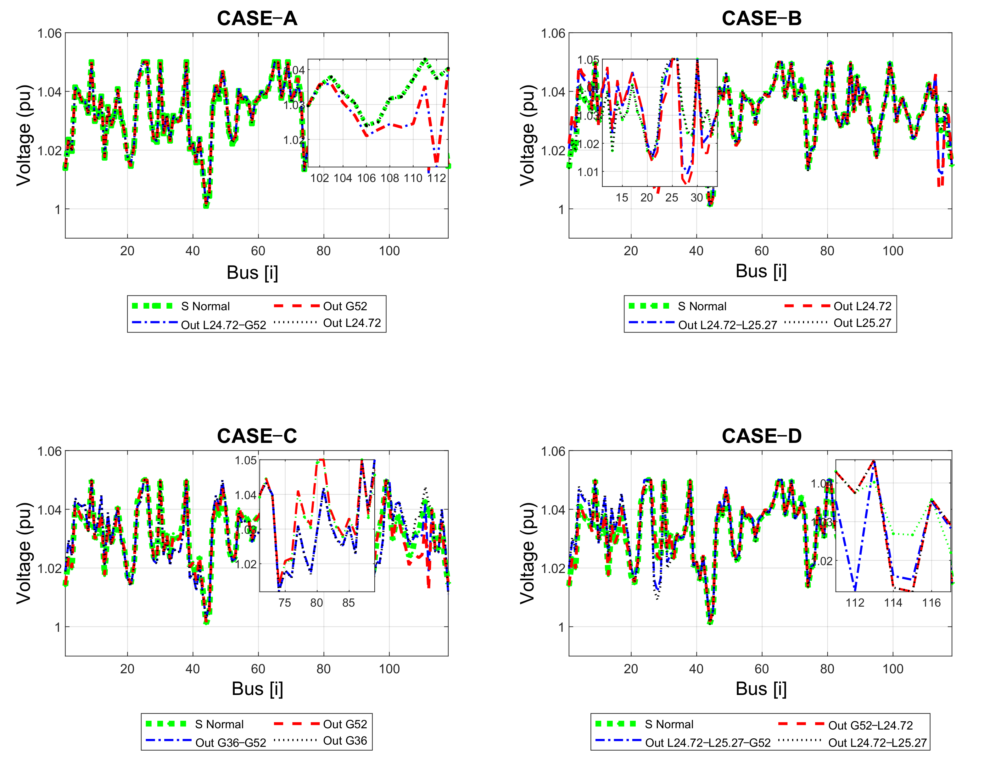
Figure 4 shows the voltage variations in the four case studies A, B, C, and D in the IEEE 118 bus system. Each case study contains the behavior of the system under a normal state which can be seen in the green line; the segmented red and black lines represent the voltage variation when disconnecting the transmission lines and the generators, respectively. Finally, the segmented blue line represents the most serious contingency. For cases, A, B, and C, contingencies N-2 are analyzed, and for case D, contingencies N-3 are taken into consideration.

• In case A, it is observed that the voltage variations when disconnecting the generator and the line are similar when disconnecting only the generator that is on bus bar 112, the variations occur only in the bus bars close to the bus where the power was from disconnected generator, and significantly in bus bar 112; as it can be seen, the voltage drops from 1.04 pu to 1.01 pu; the rest of the system does not suffer any significant damage.
• In case B, the disconnection of line 24–72 has a strong impact on the system; as it can be seen, there are significant variations in bus bars 27–28 and 113–114, as contingency N-2 generates the variation in the system. It is reduced in nodes 27–28 and 113–114; however, in nodes 1 to 27 there is a greater voltage variation in each of the buses of the electrical system.
• Case C is the worst case study when disconnecting the generators located on bus bars 80 and 112. It can be seen that there are voltage variations in all the bus bars of the system, with bus bars 80 and 112 being the most affected. In addition, it can be seen that generator 52 (connected to bus bar 112) is the one that has the greatest impact of the two elements of the electrical system, as can be seen in the red line, while generator 36 (connected to the bus bar 80) has a minor impact on the EPS while maintaining the appropriate operating limits for its operation.
• Case D contemplates the disconnection of three elements, generator number 52, lines 24–72, and 25–27. When these elements are out of service, the worst scenario is produced, having significant voltage variations on bus bars 28 and 115. In addition, there are small voltage variations from bus bars 1 to 20; this can be seen by the blue colored line.
• Case E consists of restoring the system in the face of an N-4 contingency, for which generator 52 and three transmission lines are disconnected, which are lines 24–72, 25–27, and lines 2–3.
• In case F, five elements of the EPS are disconnected, generating a contingency N-5, the first of which is generator 52. In addition, four transmission lines are disconnected: lines 24–72, 25–27, 2–3, and, finally, lines 4–9.

The variation of the voltage angle of the different study cases is observed in Figure 5.

In case A, it can be seen that when generator 52 is disconnected, it causes variation in more than half of the bus bars of the system; however, these variations do not have a considerable magnitude.

Case B presents a greater angle variation when disconnecting lines 24–72 and 25–27, these same angle changes are obtained when disconnecting only line 24–72. This is because this element has great loadability, that is, through this line, there is a greater flow of power to meet the demand.

In Case C, there is the greatest angle variation with respect to the other cases. The disconnection of two generators causes significant changes in the variables of voltage, angle, and power flow throughout the system. Despite this, the system does not fall into instability respecting operating limits. In this case, it is observed that generator 52 causes the greatest angle variation.

In case D, it can be seen that contingency N-3 is the worst scenario because it considers more than two elements that must re-enter the EPS; however, the angle variations suffered by the electrical system in each bus bar do not violate the EPS operational limits. In addition, the angle changes that occur in the system are minimal and are located in specific bus bars 28 and 115.

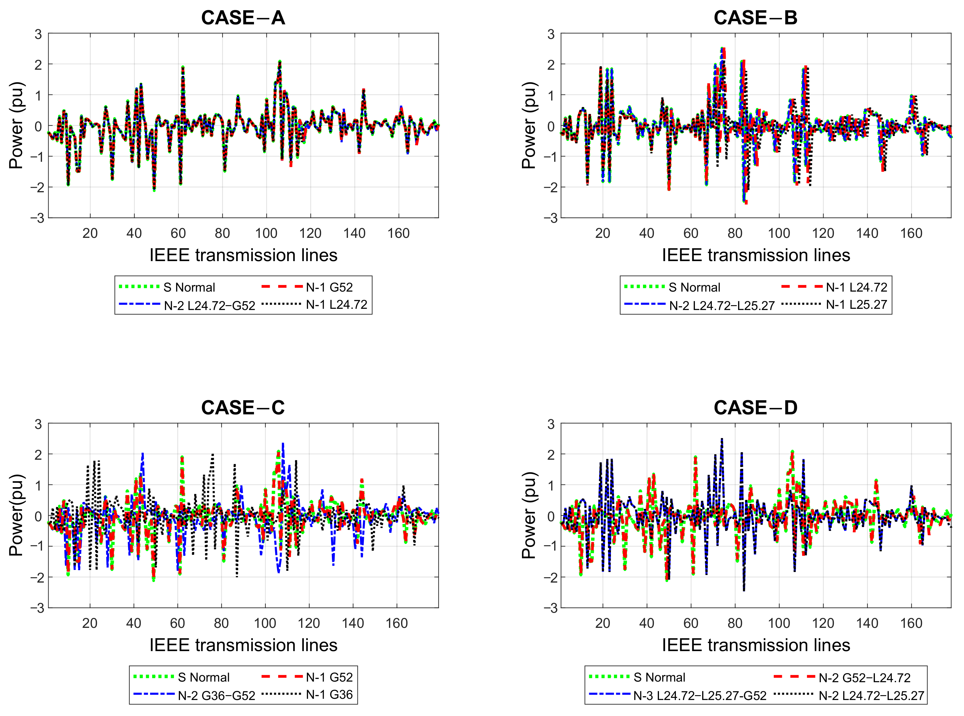
Figure 6 presents the power flow in the transmission lines according to the case studied. It is observed that in cases A and B, where the generator–line and line–line system is disconnected, the flow variations are minimal except for the disconnected lines where the power reaches zero without affecting the electrical power system.

If the system suffers the disconnection of generation units, the power flow varies significantly, as can be seen in the curves resulting from case C (see Figure 6); the green curve represents the flow of the power of the electrical system in a pre-fault state, while the curves in red, blue, and black represent the power flow when one and two generators are disconnected (post-fault), this being one of the serious cases in the present study.

The curves in case D show the power flow upon disconnection of three elements (blue curve). The disconnection of two generator–line and line–line elements is seen in the red and black lines, respectively. The N-3 contingency is another serious case in terms of power flow since it generates several peaks and significant power drops in several lines of the electrical system.

Table 1. The operating cost of generation for cases A, B, C, D, E, and F.

Solution	Normal Operation	Case A	Case B	Case C	Case D	Case E	Case F
Optimal	USD 457.8595	USD 459.1201	USD 460.0032	USD 476.3337	USD 462.7507	USD 477.6674	USD 477.7116

shows the results obtained from OPF-AC for the IEEE 118 bus bar system. By using nonlinear programming, with the help of the CONOPT solver, the optimal solution found by the proposed algorithm is presented and implemented in the Matlab–Gams interface. The optimal solution, for the proposed cases, responds to the initial restrictions of the problem that seek to minimize the operating cost of the EPS, this being the objective function. As it can be seen in Table 1, case F, which is the disconnection of five elements in the EPS, presents the highest operating costs, while case A, which is the disconnection of two elements, has the lowest operating cost within all the study cases. As more elements are disconnected from the EPS, the operating cost increases.

Table 2. Computational times for case studies.

Solution	Normal Operation	N-1	N-2	N-3	N-4	N-5
Computational Times	0.565 s	0.614 s	0.620 s	0.710 s	0.736 s	0.775 s

represents the computational time required by the machine to solve the problem posed by the proposed algorithm; when having a greater number of contingencies, the time increases exponentially. When contingencies N-5 occur, the time the machine takes is 0.775 s.

Table 3. Contingency indexes for cases A, B, C, D, E, and F in the IEEE 118 bus system.

Cases	Norm. Op	N-2	N-3	N-4	N-5
Case A	3.4254	3.4591	-	-	-
Case B	3.4254	3.7413	-	-	-
Case C	3.4254	3.824	-	-	-
Case D	3.4254	-	3.7871	-	-
Case E	3.4254	-	-	4.1704	-
Case F	3.4254	-	-	-	4.1834

represents the contingency index obtained when analyzing the different cases proposed. It can be seen that the worst contingency occurs in case F, which is contingency N-5, while the least serious contingency occurs in case A. When contingencies N-2 are generated in the EPS, there is a greater affectation in case C with a CI of 3824, which occurs when generating units 36 and 52 are disconnected.

In

Table 4. Contingency index by disconnected elements.

Element	CI
L 24-72	3.4254
G 52	3.4564
L 25-27	3.7413
L 4-9	3.8057
G 36	3.8072
L 2-3	3.8262

, the contingency index N-1 of the EPS disconnecting transmission lines and generators are ordered from the element that, when disconnecting from the EPS, has the least impact to the greatest. It can be seen that the element that has the least impact on the EPS is the line 24–72, while line 2–3 is the element that has the greatest impact when disconnecting from the EPS.

The order in which the elements must be re-entered before the generated contingencies is found in Figure 7, according to the contingency indexes found in Table A3. For case A, generator 52 must be the first to re-enter. This is carried out in order for the EPS to prepare for the re-entry of the transmission line, followed by re-entering line 24–72; in this way, the system is optimally restored. For case B, the reconnection process begins with line 24–72, followed by line 25–27.

In case C, the decision tree suggests that generator 56 must enter first, followed by generator 36. In this way, the element with the least impact enters the EPS, ensuring that the electrical system does not lose voltage stability in the face of sudden changes in the technical variables of EPS caused by contingencies. For the N-3 contingency generated, generator 52 must enter first, then line 24–72 and finally line 25–27; by following this route, the electrical system is restored in the correct way, meeting energy quality criteria and voltage stability, preventing the system from entering a voltage collapse generating a blackout.

In Figure 8, the entry of the elements for cases E and F is observed. For case E, generator 52 must be entered as the first step, followed by line 24–72, as a third step, the entry of line 25–27, finally the re-entry of line 2–3. In case F, the order of entry of the elements is first the generator 52; second, line 24–72; third, line 25–27; fourth, line 4–9; and, finally, line 2–3.

Figure 9 represents the voltage stability study that is obtained in the study cases C, D, E, and in normal operation. It can be seen that the case that presents a greater disturbance than the EPS is case C, in which generators 36 and 52 go out of operation, despite the fact that in cases D and E there are more elements that were disconnected from the system. The P–V curve was developed with a load increase $\lambda =2$ in the bar 45 of the EPS.

The stability of the system under normal conditions is represented by the red line, while for case C, stability is represented by the black lines, and for cases D and E it is represented by the lines colored green and blue, respectively. By having the IEEE 118 bar system, the reduction in the stability margin is minimal since it is a robust system. Although, with the disconnection of two generators in the EPS, a slight reduction in the stability margin is seen when disconnecting a generator and several lines, the reduction is minimal.

This work evaluates the optimal restoration of the IEEE 118 bus system under N-2 and N-3 contingencies considering generation, transmission, and transmission and generation systems. In this research, an important aspect to consider is that the proposed methodology allows to evaluate the system in case of N-M contingencies; for this purpose, cases N-4 and N-5 were created and evaluated. In addition, the model considers as restrictions the acceptable voltage limits and the difference in voltage angle between the different bus bars.

Table 5. Comparison of the proposed methodology.

Methodology	Transmission	Generation	Transmission Generation	N-M	Voltage Angle
Qiu [7]	-	X	-	-	-
Sun [10]	-	X	-	-	-
Li [4]	X	-	-	-	-
Esmaili [11]	X	-	-	-	-
Proposed	X	X	X	X	X

shows a comparison between the criteria used for this research methodology and other relevant works.

5. Conclusions

Through optimal AC power flows methodology and obtaining the contingency index, it was possible to plan the optimal restoration of the EPS. With the OPF-AC method, it was possible to determine the status of the EPS in normal operation and when contingencies were generated, which leads to obtaining the status of the main technical variables, such as voltage, angle, and power flow. On the other hand, once the technical variables were obtained, the contingency index was calculated through the voltage in the EPS bars. This technique allows establishing the magnitude of the affectation suffered by the system when one or more elements are disconnected considering the power flow; therefore, it allows determining the optimal path or route to follow for the re-entry of these elements to the EPS, fulfilling with criteria of continuity, quality, and voltage stability, observing optimal operating limits.

When applying the proposed methodology, it is important to calculate the contingency index; in this way, it is possible to determine the level of affectation suffered by the EPS when disconnecting transmission lines or generators. The higher the contingency index, the greater the variation in voltage and angular deviation. Once the results of the disconnections of the elements that went out of operation were obtained, their re-entry is planned, with the elements with the highest CI being the last to be reintegrated into the EPS and the elements with the lowest CI being the first to enter the system.

Through this research, a generic methodology was determined that allows planning the optimal restoration and can be applied in any EPS under N-M contingencies. In addition, the disconnection of elements can be generated in the generation, transmission, or both systems, giving the methodology a plus. Therefore, for the proposed work, contingencies N-2 and N-3 were carried out, which were within the objective, it was also verified that the methodology can be applied under contingencies N-4, N-5, and N-M.

6. Future Work

In the future, there are plans to develop new research in which an electrical power system that is in black start will be used as a starting case, for which an optimal restoration will be carried out in this EPS.

References

1. Adibi, M.M.; Fink, L.H. Power system restoration planning. IEEE Trans. Power Syst. 1994, 9, 22–28. [Google Scholar] [CrossRef]
2. Murinelli Pesoti, P.; De Lorenci, E.V.; Zambroni de Souza, A.C.; Lo, K.L.; Lima Lopes, B.I. Robustness Area Technique Developing Guidelines for Power System Restoration. Energies 2017, 10, 99. [Google Scholar] [CrossRef] [Green Version]
3. Zhang, H.; Li, G.; Yuan, H. Collaborative Optimization of Post-Disaster Damage Repair and Power System Operation. Energies 2018, 11, 2611. [Google Scholar] [CrossRef] [Green Version]
4. Li, C.; He, J.; Zhang, P.; Xu, Y. A Novel Sectionalizing Method for Power System Parallel Restoration Based on Minimum Spanning Tree. Energies 2017, 10, 948. [Google Scholar] [CrossRef] [Green Version]
5. Carrión, D.; Francisco, J.; Paul, M. Revisión para la restauración optima de la operación del sistema eléctrico basado en criterios de calidad de energía y estabilidad. Revista de I+D Tecnológico 2021, 17, 9. [Google Scholar] [CrossRef]
6. Jiang, P.; Chen, Q. An Optimal Source-Load Coordinated Restoration Method Considering Double Uncertainty. Energies 2018, 11, 558. [Google Scholar] [CrossRef] [Green Version]
7. Qiu, F.; Li, P. An Integrated Approach for Power System Restoration Planning. Proc. IEEE 2017, 105, 1234–1252. [Google Scholar] [CrossRef]
8. Ganganath, N.; Wang, J.V.; Xu, X.; Cheng, C.; Tse, C.K. Agglomerative Clustering-Based Network Partitioning for Parallel Power System Restoration. IEEE Trans. Ind. Inform. 2018, 14, 3325–3333. [Google Scholar] [CrossRef] [Green Version]
9. Goo, B.; Jung, S.; Hur, J. Development of a Sequential Restoration Strategy Based on the Enhanced Dijkstra Algorithm for Korean Power Systems. Appl. Sci. 2016, 6, 435. [Google Scholar] [CrossRef] [Green Version]
10. Sun, R.; Liu, Y.; Zhu, H.; Azizipanah-Abarghooee, R.; Terzija, V. A network reconfiguration approach for power system restoration based on preference-based multiobjective optimization. Appl. Soft Comput. 2019, 83, 105656. [Google Scholar] [CrossRef]
11. Esmaili, M.R.; Khodabakhshian, A.; allah Hooshmand, R.; Siano, P. A new coordinated design of sectionalizing scheme and load restoration process considering reliability of transmission system. Int. J. Electr. Power Energy Syst. 2018, 102, 23–37. [Google Scholar] [CrossRef]
12. Escobar, A.; Gallego, L. Análisis estático de contingencias de potencia activa en sistemas eléctricos de potencia. Sci. Technol. 2004, 1–6. [Google Scholar] [CrossRef]
13. Escobar, Z.A.; Gallego, L. Análisis estático de contingencias de voltaje en sistemas eléctricos de potencia. Sci. Technol. 2004, 1–6. [Google Scholar] [CrossRef]
14. Escudero Delgado, P.; Carrión Galarza, D. Expansión de un sistema de transmisión mediante LOPF-AC. INGE CUC 2018, 14, 116–125. [Google Scholar] [CrossRef]
15. Li, Y.; Li, Y. Two-Step Many-Objective Optimal Power Flow Based on Knee Point-Driven Evolutionary Algorithm. Processes 2018, 6, 250. [Google Scholar] [CrossRef] [Green Version]
16. Li, Z.; Cao, Y.; Dai, L.V.; Yang, X.; Nguyen, T.T. Optimal Power Flow for Transmission Power Networks Using a Novel Metaheuristic Algorithm. Energies 2019, 12, 4310. [Google Scholar] [CrossRef] [Green Version]
17. Masache, P.; Carrión, D. Estado del Arte de conmutación de líneas de transmisión con análisis de contingencias. Revista de I+D Tecnológico 2019, 15, 98–106. [Google Scholar] [CrossRef] [Green Version]
18. Poyrazoglu, G.; Oh, H. Optimal Topology Control With Physical Power Flow Constraints and N-1 Contingency Criterion. IEEE Trans. Power Syst. 2015, 30, 3063–3071. [Google Scholar] [CrossRef]
19. Duque, F.G.; de Oliveira, L.W.; de Oliveira, E.J.; Augusto, A.A. State estimator for electrical distribution systems based on an optimization model. Electr. Power Syst. Res. 2017, 152, 122–129. [Google Scholar] [CrossRef]
20. Blood, E.A.; Krogh, B.H.; Ilic, M.D. Electric power system static state estimation through Kalman filtering and load forecasting. In Proceedings of the 2008 IEEE Power and Energy Society General Meeting—Conversion and Delivery of Electrical Energy in the 21st Century, Pittsburgh, PA, USA, 20–24 July 2008; pp. 1–6. [Google Scholar] [CrossRef]
21. Armaghani, S.; Hesami Naghshbandy, A.; Shahratash, S.M. Application of a new fast analytical approach for post-contingency state estimation of “N-1” transmission line outage in online vulnerability assessment of large-scale transmission networks with wind power resources. Int. J. Electr. Power Energy Syst. 2020, 123, 106304. [Google Scholar] [CrossRef]
22. Banerjee, T.; Chen, Y.C.; Dominguez-Garcia, A.D.; Veeravalli, V.V. Power system line outage detection and identification—A quickest change detection approach. In Proceedings of the 2014 IEEE International Conference on Acoustics, Speech and Signal Processing (ICASSP), Florence, Italy, 4–9 May 2014; pp. 3450–3454. [Google Scholar] [CrossRef]
23. Miller, P.; Waltz, B.; Chadbourne, C. Transmission line measuring device and method for connectivity and monitoring Hubbel Incorporated, (US) Patent. US9767685B2, 9 September 2017. [Google Scholar]
24. Bolshev, V.; Vinogradov, A.; jasiński, M.; Sikorski, T.; Leonowicz, Z.; Gono, R. Monitoring the Number and Duration of Power Outages and Voltage Deviations at Both Sides of Switching Devices. IEEE Access 2020, 8, 137174–137184. [Google Scholar] [CrossRef]
25. Yang, Y. Power Line Sensor Networks for Enhancing Power Line Reliability and Utilization; Georgia Institute of Technology: Atlanta, GA, USA, 2011; p. 264. Available online: http://hdl.handle.net/1853/41087 (accessed on 1 February 2022).
26. Andersson, C.; Solem, J.E.; Eliasson, B. Classification of power system stability using support vector machines. In Proceedings of the IEEE Power Engineering Society General Meeting, San Francisco, CA, USA, 16 June 2005; Volume 1, pp. 650–655. [Google Scholar] [CrossRef]
27. Wiszniewski, A. New Criteria of Voltage Stability Margin for the Purpose of Load Shedding. IEEE Trans. Power Deliv. 2007, 22, 1367–1371. [Google Scholar] [CrossRef] [Green Version]
28. Liu, Y.; Fan, R.; Terzija, V. Power system restoration: A literature review from 2006 to 2016. J. Mod. Power Syst. Clean Energy 2016, 4, 332–341. [Google Scholar] [CrossRef] [Green Version]
29. Sharma, D.; Lin, C.; Luo, X.; Wu, D.; Thulasiraman, K.; Jiang, J.N. Advanced techniques of power system restoration and practical applications in transmission grids. Electr. Power Syst. Res. 2020, 182, 106238. [Google Scholar] [CrossRef]
30. Braun, M.; Brombach, J.; Hachmann, C.; Lafferte, D.; Klingmann, A.; Heckmann, W.; Welck, F.; Lohmeier, D.; Becker, H. The Future of Power System Restoration: Using Distributed Energy Resources as a Force to Get Back Online. IEEE Power Energy Mag. 2018, 16, 30–41. [Google Scholar] [CrossRef]
31. Mezghani, I.; Misra, S.; Deka, D. Stochastic AC Optimal Power Flow: A Data-Driven Approach. Electr. Power Syst. Res. 2020, 189, 106567. [Google Scholar] [CrossRef]
32. Venzke, A.; Chatzivasileiadis, S.; Molzahn, D.K. Inexact Convex Relaxations for AC Optimal Power Flow: Towards AC Feasibility. Electr. Power Syst. Res. 2020, 187, 106480. [Google Scholar] [CrossRef]
33. Rokrok, E.; Shafie-khah, M.; Siano, P.; Catalão, J.P.S. A Decentralized Multi-Agent-Based Approach for Low Voltage Microgrid Restoration. Energies 2017, 10, 1491. [Google Scholar] [CrossRef] [Green Version]
34. Louca, R.; Bitar, E. Robust ac optimal power flow. IEEE Trans. Power Syst. 2019, 34, 1669–1681. [Google Scholar] [CrossRef] [Green Version]
35. Kundur, P.; Paserba, J.; Vitet, S. Overview on definition and classification of power system stability. In Proceedings of the CIGRE/IEEE PES International Symposium Quality and Security of Electric Power Delivery Systems—CIGRE/PES 2003, Montreal, QC, Canada, 8–10 October 2003; pp. 1–4. [Google Scholar] [CrossRef]
36. Shuai, Z.; Shen, C.; Liu, X.; Li, Z.; Shen, Z.J. Transient Angle Stability of Virtual Synchronous Generators Using Lyapunov’s Direct Method. IEEE Trans. Smart Grid 2019, 10, 4648–4661. [Google Scholar] [CrossRef]
37. Castellanos, R. Determinación de límites de transmisión en sistemas eléctricos de potencia. Ingeniería, Investigación y Tecnología 2014, 15, 271–286. [Google Scholar] [CrossRef] [Green Version]
38. Masetti, C. Revision of European Standard EN 50160 on power quality: Reasons and solutions. In Proceedings of the 14th International Conference on Harmonics and Quality of Power—ICHQP 2010, Bergamo, Italy, 26–29 September 2010; pp. 1–7. [Google Scholar] [CrossRef]
39. Malakar, S.; Maharana, M.K. Network contingency ranking using analytic hierarchy process to calculate unequal importance factors for static severity indices. In Proceedings of the Michael Faraday IET International Summit 2015, Kolkata, India, 12–13 September 2015; pp. 249–255. [Google Scholar] [CrossRef]
40. Mishra, A.; Gundavarapu, V.N.K. Contingency management of power system with Interline Power Flow Controller using Real Power Performance Index and Line Stability Index. Ain Shams Eng. J. 2016, 7, 209–222. [Google Scholar] [CrossRef] [Green Version]
41. Carrión, D.; García, E.; Jaramillo, M.; González, J.W. A Novel Methodology for Optimal SVC Location Considering N-1 Contingencies and Reactive Power Flows Reconfiguration. Energies 2021, 14, 6652. [Google Scholar] [CrossRef]
42. Fernandez-Porras, P.; Panteli, M.; Quiros-Tortos, J. Intentional Controlled Islanding: When to Island for Power System Blackout Prevention. IET Gener. Transm. Distrib. 2018, 12. [Google Scholar] [CrossRef] [Green Version]
Figure 1. Proposed solution architecture.
Energies 15 02062 g001
Figure 2. IEEE 118 bus system [42].
Energies 15 02062 g002
Figure 3. Solution methodology for the optimal restoration of EPS.
Energies 15 02062 g003
Figure 4. Voltages on IEEE 118 bus bars system subjected to contingencies.
Energies 15 02062 g004
Figure 5. Angular deviation in the IEEE 118 system bus bars subjected to contingencies.
Energies 15 02062 g005
Figure 6. Power flow in transmission lines for the different study cases.
Energies 15 02062 g006
Figure 7. Decision tree for the entry of EPS elements, cases A, B, C, and D.
Energies 15 02062 g007
Figure 8. Decision tree for the entry of EPS elements, cases E and F.
Energies 15 02062 g008
Figure 9. Voltage stability curve, P–V.
Energies 15 02062 g009