A Sensitivity-Based Three-Phase Weather-Dependent Power Flow Algorithm for Networks with Local Voltage Controllers

Abstract

Local voltage controllers (LVCs) are important components of a modern distribution system for regulating the voltage within permissible limits. This manuscript presents a sensitivity-based three-phase weather-dependent power flow algorithm for distribution networks with LVCs. More specifically, the proposed algorithm has four distinct characteristics: (a) it considers the three-phase unbalanced nature of distribution systems, (b) the operating state of LVCs is calculated using sensitivity parameters having accelerated convergence, (c) it considers the precise switching sequence of LVCs based on their reaction time delays, and (d) the nonlinear influence of weather variations in the power flow is also taken into consideration. Simulations and validation results presented indicate that the proposed approach outperforms other existing algorithms with respect to the accuracy and speed of convergence, thus making it a promising power flow tool for accurate distribution system analysis.

1. Introduction

Local voltage controllers (LVCs) are important components in modern distribution networks. These are physical apparatus such as on-load tap changer transformer (OLTC), step voltage regulator (SVR), switched capacitor, distributed generator (DG), which regulate the voltage of a specific bus within permissible limits [1,2,3].

For safe, reliable, and efficient operation, distribution management systems (DMS) regularly carry out state estimation and optimization functions such as Volt/Var control (VVC) and optimal feeder reconfiguration (OFR). These functions require the online execution of power flow, by generating what-if scenarios. As soon as an assessment of the network’s state is estimated via distribution system state estimation [4], DMS optimization functions calculate new switching states for the local controllers to optimize the network operation. The real-time power flow constitutes an integral part of VVC and OFR functions. More specifically, it is applied to estimate how the switching actions of LVCs affect the performance of the network, and accordingly, it is sent (or not) for execution via SCADA [2]. As a result, precise and fast computation of power flow in networks with LVCs is crucial for the effective execution of DMS optimization functions and state estimation of distribution networks.

1.1. Challenges of Incorporating LVCs in Power Flow Computation

Although several power flow methods have been presented in the literature for simulating the steady state of distribution networks, the overwhelming majority of them has not considered the exact operation of LVCs e.g., SVRs, OLTCs, switched capacitors [5,6,7,8,9].

For the incorporation of LVCs into the power flow, there are two common approaches: the error-feedback adjustment method and the automatic adjustment method [1,2,10]. In the error feedback methods, the control variables e.g., taps of SVR/OLTCs, states of capacitors and reactive power of DGs are updated after each iteration of power flow, based on the deviation of the regulated voltage from its target value. For instance, after the execution of each power flow iteration, the deviation of the voltage value of each LVC is computed and the respective tap or switching state is updated accordingly. The error feedback methods result in high oscillations of the power system states if the interactions between the LVCs are strong [2,3].

On the other hand, in automatic adjustment methods, the control variables are incorporated into the power flow equations and are solved simultaneously. This method is usually applied in the Newton–Raphson (NR) approach, in which the control variables are incorporated into the Jacobian matrix. Although the interactions between the control variables are considered in automatic adjustment methods and the oscillations are avoided, the discreteness of control variables is ignored, e.g., taps of transformers. The variables are discretized to the nearest discrete value after the power flow has converged, resulting in final voltage solutions, which may lie outside the permissible limits [2].

Another important challenge when incorporating LVCs into the power flow computation is the existence of multiple power flow solutions resulting from the different ways that a system state is reached. More specifically, LVCs are usually switched with different switching delays [1]. For example, an SVR placed near the substation may react faster in a voltage violation than an SVR placed at a farther distance. Furthermore, LVCs are set with different voltage bandwidths, inside which the state of LVC is unvaried. Due to the different reaction sequence of LVCs, the power flow could yield multiple steady state solutions, with all of them satisfying the voltage constraints. As a result, the actual switching sequence of LVCs should be considered according to their time delays and bandwidths, in order to compute the most probable power flow solution [1,2].

Another important challenge is the variety of operational modes of DGs. They may operate in constant voltage mode (modeled as PV nodes) [3] or in droop Q(V) mode according to the newly developed standard IEEE Std 1547-2018 from March 2018 [11,12,13,14,15,16,17,18]. In both cases, they interact with the other LVCs. Finally, the DGs may operate in different configurations e.g., 3-wire or 4-wire and may generate different voltage profiles e.g., balanced voltage or balanced current, which significantly affects the power flow results [14]. Therefore, precise modeling of the DGs is also required, which should simulate the actual operational characteristics of the DGs as well as the interactions with the other LVCs.

1.2. Literature Review

Two NR-based automatic adjustment methods are proposed in [15,16] by incorporating the LVCs into the Jacobian matrix. Another automatic adjustment method is proposed in [17], where the authors incorporate the LVC variables into the admittance matrix of the system forming a hybrid model, in which the LVC variables are solved simultaneously with the power flow.

An error-feedback method is proposed in [10], by adjusting the LVC variables after each iteration of power flow. However, a possible hunting oscillation may be observed between different adjustments due to the interaction of LVCs. To overcome the hunting, authors in [3] adopted sensitivity parameters that consider the interactions between the LVCs in single-phase formulation. In this way, the oscillations between consecutive power flow iterations are reduced, and the speed and robustness of the power flow solution are enhanced. All the aforementioned works ignore the time delays of LVCs, thus the actual switching sequence of the LVCs is not represented. As a result, the aforementioned power flow approaches do not yield the most probable power flow solution but rather a random one.

The time delays of LVCs were introduced for the first time into the power flow studies in [1]. The authors divided the LVCs into different delay groups. The LVCs with the fastest reaction belong to the first group, while the slowest ones belong to the last group. A similar division of LVCs into delay groups is applied in [18]. The method of [1] was improved in [2] by introducing sensitivity parameters to accelerate the convergence of the power flow. Authors in [2] claim that the power flow methods of [1,2] calculate precisely the power flow by estimating the most probable switching states of LVCs. However, it will be shown through dynamic simulations in Section 7 of this paper that none of the above-mentioned references calculate precisely the power flow since they ignore the actual switching sequence of LVCs. Furthermore, all methods described above (except [16,18]) neglect the network unbalances and the variety of DG operational modes investigating only single-phase networks.

1.3. Technical Contribution of This Paper

A lot of effort has been put so far by the researchers to study the optimal operation of LVCs in distribution networks e.g., [11,13,19,20,21,22,23,24,25,26]. However, power flow computation in distribution networks with LVCs has not been extensively studied, and scope to improve remains. This manuscript contributes by proposing an error-feedback power flow method with the following distinct characteristics:

• In contrast to the existing literature, the proposed method is a three-phase algorithm, which considers the network’s unbalances. Moreover, the proposed power flow method accurately simulates various DG operational modes.
• It calculates the actual switching sequence of LVCs based on their time delays. It is shown through dynamic simulation in Simulink that the proposed power flow method produces more accurate results than the methods of [1,2,3] which are considered the state of the art in the steady-state modeling of LVCs.
• Three-phase self- and mutual-sensitivity parameters are derived relating the control variables (e.g., taps of OLTC and SVRs, capacitors, reactive power of DGs) with the regulated voltages of the network. The sensitivity parameters are then applied in the proposed algorithm to accelerate the convergence of the power flow, reducing significantly the computation time. This property is very important since power flow computation with LVCs is widely applied in real-time DMS applications, in which time is a crucial factor.
• Unlike existing approaches, the proposed approach considers the weather and magnetic effects, which have a great influence on the impedance of overhead conductors [27,28], thus significantly affecting the power flow results and the switching state of LVCs.

2. Weather and Magnetic Dependent Power Flow

In this section, the weather and magnetic dependent power flow solver applied in this manuscript is briefly described. The algorithm utilizes the nonlinear thermal equations of IEEE Std 738-2012 for calculating the conductor temperature and the nonlinear impedance-temperature-current relation proposed in [27] for calculating the conductor impedance. The power flow is solved using the implicit Z_BUS method [27] and matrix decomposition [29].

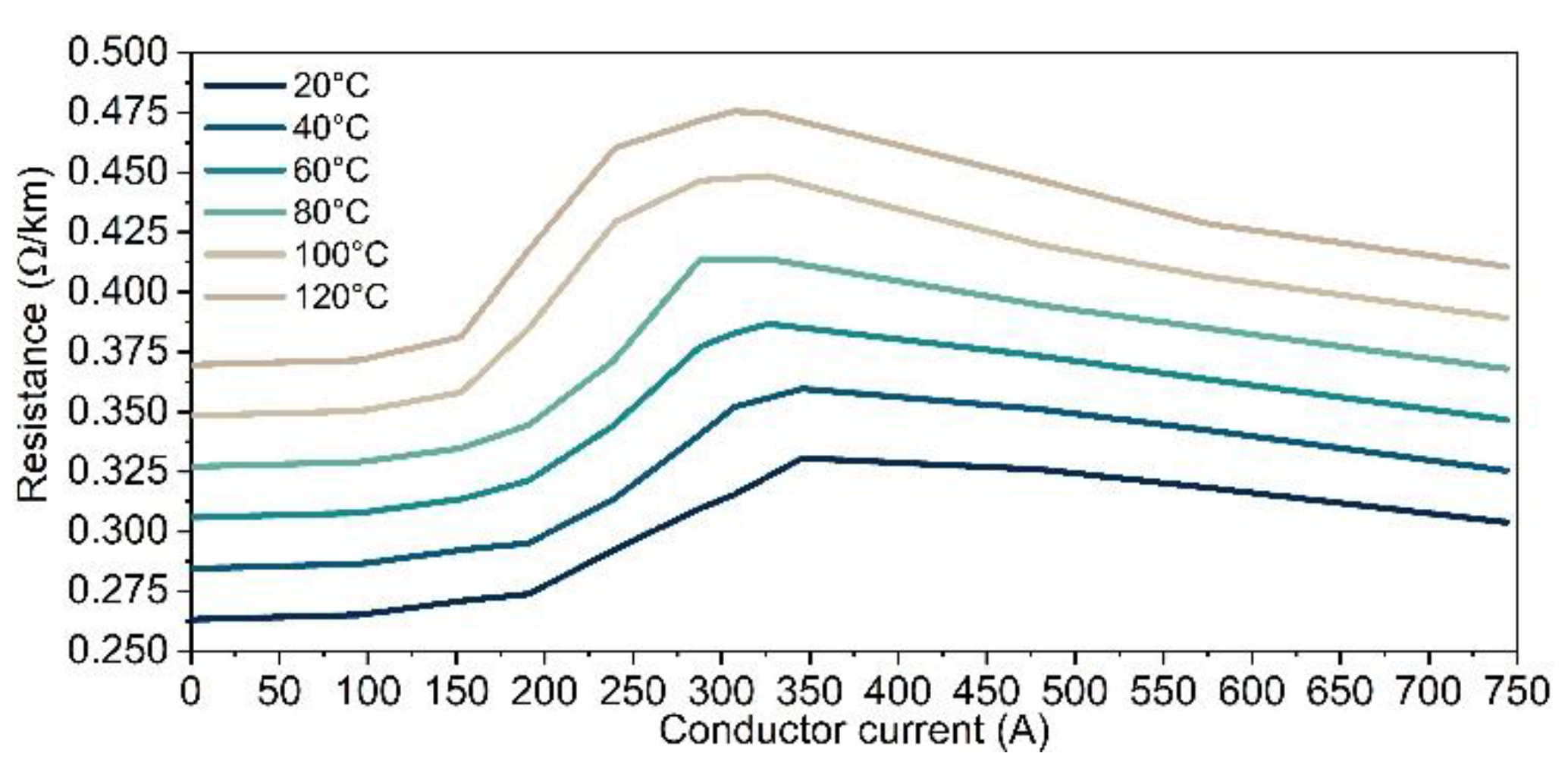
2.1. Thermal Modeling of Overhead Conductors

The temperature of an overhead conductor can be calculated from the nonlinear heat-balance equation of IEEE Std 738-2012 [30]. The nonlinear heat-balance equation is as follows:

$$Q_c+Q_r=Q_s+Q_j$$

(1)

where $Q_c$ is the convective heat loss, $Q_r$ is the radiative heat loss, $Q_s$ is the heat gain due to solar radiation, and $Q_j$ is the heat gain due to joule heating.

The nonlinear heat-balance Equation (1) is solved with Newton’s method to obtain the conductor temperature ($T_c$), for any amount of current flow under any given weather condition experienced by the conductor (more details are given in [27,30]).

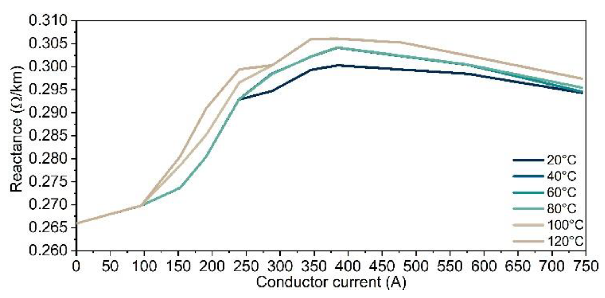
2.2. Modeling of the Magnetic Effects

IEEE Std 738-2012 [30] assumes a simplified linear resistance-temperature relationship that ignores the nonlinearities arising from the magnetic effects in the core of the conductors. Practically, both ACSR (aluminum conductor steel reinforced) and AAC (all-aluminum conductor) overhead conductors consist of many aluminum wires stranded helically around a central core. Thus, the current flowing through these wires follows a helical path resulting in an additional longitudinal magnetic field in the core of the conductor, and thus, increasing the losses and impedance of conductor [27]. This effect is most pronounced in single-layer ACSR conductors (e.g., below 400 A [31]).

An algorithm to accurately calculate the impedance of overhead conductors based on the conductor temperature (calculated by Equation (1) in Section 2.1) and current (calculated by the power flow in Section 2.3) is described in [27].

2.3. Power Flow Solver Using Matrix Decomposition

The equation of implicit Z-Bus power flow is described by (2) below:

$${\left[\begin{array}{c}{\mathit{V}}_{\mathbf{1}}\\ ⋮\\ {\mathit{V}}_{\mathit{m}}\end{array}\right]}^{\left(k+1\right)}={\left[\begin{array}{ccc}{\mathit{{\rm Y}}}_{\mathbf{11}}& \cdots & {\mathit{{\rm Y}}}_{\mathbf{1}\mathit{m}}\\ ⋮& \ddots & ⋮\\ {\mathit{{\rm Y}}}_{\mathit{m}\mathbf{1}}& \cdots & {\mathit{{\rm Y}}}_{\mathit{m}\mathit{m}}\end{array}\right]}^{-1}\left({\left[\begin{array}{c}{\mathit{I}}_{\mathbf{1}}\\ ⋮\\ {\mathit{I}}_{\mathit{m}}\end{array}\right]}^k-\left[\begin{array}{c}{\mathit{Y}}_{\mathbf{10}}\\ ⋮\\ {\mathit{Y}}_{\mathit{m}\mathbf{0}}\end{array}\right]·{\mathit{V}}_{\mathbf{0}}\right)$$

(2)

where k is the iteration number, ${\mathit{V}}_{\mathit{i}}$ and ${\mathit{I}}_{\mathit{i}}$ are the vectors including the three-phase complex voltages and currents of bus i. ${\mathit{{\rm Y}}}_{\mathit{i}\mathit{j}}$ is the self- or mutual-admittance matrix between bus i and j. ${\mathit{V}}_{\mathbf{0}}$ is the voltage of the slack bus. Equation (2) is iteratively solved until convergence. More details are provided in [27].

In order to avoid time-consuming repetitive factorizations of the Z_BUS matrix of Equation (2), as a result of the impedance variation, the matrix decomposition technique is applied on the Z_BUS matrix, as follows:

$${\left[\begin{array}{ccc}{\mathit{{\rm Y}}}_{\mathbf{11}}& \cdots & {\mathit{{\rm Y}}}_{\mathbf{1}\mathit{m}}\\ ⋮& \ddots & ⋮\\ {\mathit{{\rm Y}}}_{\mathit{m}\mathbf{1}}& \cdots & {\mathit{{\rm Y}}}_{\mathit{m}\mathit{m}}\end{array}\right]}^{-1}={\mathit{K}}^T·\left[\begin{array}{ccc}{\mathit{Z}}_{\#\mathbf{1}}& \mathbf{0}& \mathbf{0}\\ \mathbf{0}& \ddots & \mathbf{0}\\ \mathbf{0}& \mathbf{0}& {\mathit{Z}}_{\#\mathit{m}}\end{array}\right]·\mathit{K}$$

(3)

where the branch-path incidence matrix $\mathit{K}$ is given in [29]. ${\mathit{Z}}_{\#\mathbf{i}}$ for $i\in \left\{1, \dots , m\right\}$ includes the 3 × 3 impedance matrix of each three-phase line section. More details are provided in [29].

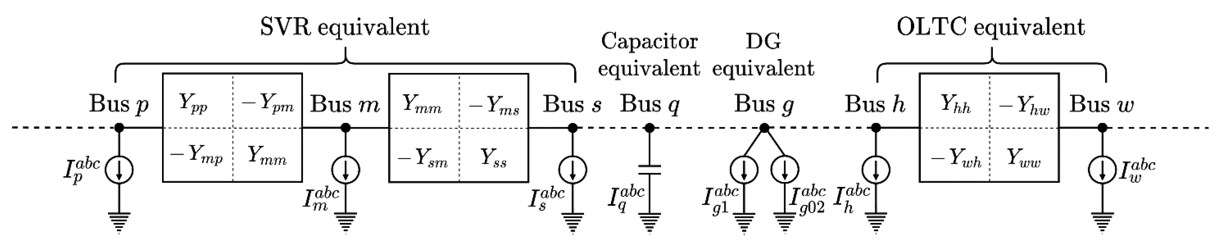
3. Modeling of Local Voltage Controllers

The modeling and operational modes of LVCs are briefly described below.

3.1. Switched Capacitors

Switched capacitors in distribution networks usually operate in voltage or reactive power control. In voltage control mode, the controller switches the capacitor ON when the measured voltage is less than a minimum value and OFF when it is more than a maximum value [32]. In reactive power mode, the state of capacitor depends on the reactive power flowing through the controlled line.

3.2. Step Voltage Regulators

A three-phase SVR model is proposed in [33], the equivalent of which is depicted in Figure 1. It is a 3-bus equivalent that simulates the taps as current sources, enabling the construction of sensitivity parameters relating the tap variables with the voltages, as explained in the next section.

3.3. On-Load Tap Changing Transformers

A three-phase OLTC transformer model is presented in [34] and its 2-bus equivalent circuit is shown in Figure 1. The taps are simulated as current sources in a similar sense as in SVRs.

3.4. Distributed Generators

The steady state modeling of DGs is usually categorized depending on the generated voltage/current profile as well as the power profile, as follows:

• Voltage and current profile: Electronically coupled DGs can generate balanced phase-to-phase voltage, balanced phase-to-neutral voltage, or balanced current. On the opposite, synchronous generators present nonzero finite negative- and zero-sequence admittances, and therefore, they generate unbalanced voltages and currents [14].
• Power profile: DGs can operate in constant PQ, constant PV (conventional PV bus modeling), or constant P-Q(V) mode [12,13]. The first case does not pose any challenge to the power flow computation since the DG is simply modeled as a negative constant power load. However, DGs with controllable reactive power may interact with the other LVCs increasing the number of power flow iterations or even leading to divergence.

4. An Algorithm for Estimating the Actual Switching Sequence of LVCs

4.1. Time Delays of LVCs

LVCs in a network are regulated to react with pre-defined time delays. This occurs in order to coordinate the operation of LVCs and to avoid unnecessary switchings, due to temporary voltage violations.

Switching capacitors, for example, are set intentionally with a time delay such that the capacitor switching is activated after a pre-defined time delay from the instant of voltage (or reactive power) violation. In the following, the delay of capacitor $i$ is denoted as ${\mathsf{{\rm T}}}_{\mathrm{delay}\left(\mathrm{i}\right)}^{\mathrm{cap}}$.

Similarly, SVR and OLTC step the voltage up or down when a voltage violation occurs beyond a pre-defined bandwidth, considering a pre-specified time delay. For instance, once a voltage violation at the supervised bus is noticed, the counter of LVC starts counting. The first step-up/down switching action is executed as soon as the counter reaches the intentional time delay. If the voltage remains outside the bandwidth, additional step-up/down actions are executed with a mechanical delay. The intentional and mechanical delays of SVR $i$ and OLTC $i$ are denoted here as ${\mathsf{{\rm T}}}_{\mathrm{delay}\_\mathrm{int}\left(\mathrm{i}\right)}^{\mathrm{svr}}$, ${\mathsf{{\rm T}}}_{\mathrm{delay}\_\mathrm{mech}\left(\mathrm{i}\right)}^{\mathrm{svr}}$, ${\mathsf{{\rm T}}}_{\mathrm{delay}\_\mathrm{int}\left(\mathrm{i}\right)}^{\mathrm{oltc}}$, ${\mathsf{{\rm T}}}_{\mathrm{delay}\_\mathrm{mech}\left(\mathrm{i}\right)}^{\mathrm{oltc}}$. DGs are assumed to react instantaneously to any load/generation variation [11,20,22,23].

Switching capacitors, SVRs, and OLTCs can operate in two different ways: (a) their three phases are independently controlled, namely every phase has its own LVC, or (b) The three phases are controlled simultaneously by the same LVC [35,36,37].

4.2. Presentation of the Proposed Algorithm

Let us firstly assume a network with $N$ local controllers, which control the switching capacitors, SVRs and OLTCs. Let us further assume that ${\mathrm{N}}_{\mathrm{SVR}}$ of them control an SVR (one or more phases depending on whether the three phases are independently or simultaneously controlled), ${\mathrm{N}}_{\mathrm{OLTC}}$ of them control an OLTC, while ${\mathrm{N}}_{\mathrm{CAP}}$ of them control a capacitor so that ${\mathrm{N}}_{\mathrm{SVR}}\subseteq \mathrm{N}$, ${\mathrm{N}}_{\mathrm{OLTC}}\subseteq \mathrm{N}$ and ${\mathrm{N}}_{\mathrm{CAP}}\subseteq \mathrm{N}$ as well as ${\mathrm{N}}_{\mathrm{SVR}}+{\mathrm{N}}_{\mathrm{OLTC}}+{\mathrm{N}}_{\mathrm{CAP}}=\mathrm{N}$.

• INITIALIZATION: Initialize the taps of SVRs and OLTCs as well as the capacitor states, and set ${\mathrm{T}}_{\mathrm{prior}\left(\mathrm{i}\right)}\to \infty$ ∀$\mathrm{i}\in \mathrm{N}$. Specify the voltage bandwidth ($B{W}_i$), the time delays ${\mathsf{{\rm T}}}_{\mathrm{delay}\left(\mathrm{i}\right)}^{\mathrm{cap}}$, ${\mathsf{{\rm T}}}_{\mathrm{delay}\_\mathrm{int}\left(\mathrm{i}\right)}^{\mathrm{svr}}$, ${\mathsf{{\rm T}}}_{\mathrm{delay}\_\mathrm{mech}\left(\mathrm{i}\right)}^{\mathrm{svr}}$, ${\mathsf{{\rm T}}}_{\mathrm{delay}\_\mathrm{int}\left(\mathrm{i}\right)}^{\mathrm{oltc}}$, ${\mathsf{{\rm T}}}_{\mathrm{delay}\_\mathrm{mech}\left(\mathrm{i}\right)}^{\mathrm{oltc}}$ ∀$i\in N$.
• STEP 1: Compute the power flow considering the DGs. In this step, the power flow is executed until convergence considering the operational mode of DGs (refer to Section 3.4).
• STEP 2: Calculate ${\mathrm{T}}_{\mathrm{prior}\left(\mathrm{i}\right)}$ for each controller $i\in \mathrm{N}$ as follows:

  $$\begin{array}{l}{T}_{prior\left(i\right)}\\ =\{\begin{array}{ll}\mathit{min}\left(T_{delay\left(i\right)}^{cap},T_{prior\left(i\right)}\right)& if \left|V_i-V_{set\left(i\right)}\right|>\frac{B{W}_i}{2} and i\in N_{CAP}\\ \mathit{min}\left(T_{delay\_int\left(i\right)}^{svr},T_{prior\left(i\right)}\right)& if \left|V_i-V_{set\left(i\right)}\right|>\frac{B{W}_i}{2} and i\in N_{SVR}\\ \mathit{min}\left(T_{delay\_int\left(i\right)}^{oltc},T_{prior\left(i\right)}\right)& if \left|V_i-V_{set\left(i\right)}\right|>\frac{B{W}_i}{2} and i\in N_{OLTC}\\ \infty & otherwise\end{array}\end{array}$$

  (4)

The function $min\left(x,y\right)$ in Equation (4) returns the lowest value between x and y. $V_i$ and $V_{set\left(i\right)}$ are the calculated (from step 1) and desired voltage magnitude of local controller $i$, respectively.

If the voltage $V_i$ is outside the limits, the priority indicator ${\mathrm{T}}_{\mathrm{prior}\left(\mathrm{i}\right)}$ is updated taking the lowest value between the intentional delay of the local controller $i$ and the current value of ${\mathrm{T}}_{\mathrm{prior}\left(\mathrm{i}\right)}$. If the voltage is inside limits, ${\mathrm{T}}_{\mathrm{prior}\left(\mathrm{i}\right)}$ is set to infinite.

• STEP 3: Find the controller $j$ with the minimum priority indicator such that ${\mathrm{T}}_{\mathrm{prior}\left(\mathrm{j}\right)}\le {\mathrm{T}}_{\mathrm{prior}\left(\mathrm{i}\right)}$ ∀$i\in N$. Then, for each controller $i\in N$, set ${\mathrm{T}}_{\mathrm{prior}\left(\mathrm{i}\right)}={\mathrm{T}}_{\mathrm{prior}\left(\mathrm{i}\right)}-{\mathrm{T}}_{\mathrm{prior}\left(\mathrm{j}\right)}$. As shown, the priority indicator with the lowest value is subtracted from the other priority indicators. Consequently, controller $j$ with the minimum ${\mathrm{T}}_{\mathrm{prior}\left(\mathrm{j}\right)}$ becomes 0 and it will undergo switching action. It should be noted that if one or more controllers have the same priority indicator value with controller $j$, their priority indicator also becomes 0 in this step, and hence, they will also undergo switching actions simultaneously.

This step prioritizes the switching actions based on their time settings. A zero ${\mathrm{T}}_{\mathrm{prior}\left(\mathrm{j}\right)}$ value means that the counter of LVC j has reached its time delay, and therefore, a switching action should be undertaken from jth LVC.

• STEP 4: In this step, controller $j$ with the minimum ${\mathrm{T}}_{\mathrm{prior}\left(\mathrm{j}\right)}$ value, undergoes switching action according to Algorithm 1.

  Algorithm 1. Switching Logic 1

  If$j\in N_{SVR}$or$j\in N_{OLTC}$then { $Ta{p}_j=\{ \begin{array}{c}Ta{p}_j+1 if V_j<V_{set\left(j\right)}-\frac{B{W}_j}{2} and Ta{p}_j<Ta{p}_{max} \\ Ta{p}_j-1 if V_j>V_{set\left(j\right)}+\frac{B{W}_j}{2} and Ta{p}_{min}<Ta{p}_j \\ Ta{p}_j otherwise \end{array}$ } If$j\in N_{CAP}$ then { $Ca{p}_j=\{\begin{array}{c} ON if V_j<V_{set\left(j\right)}-\frac{B{W}_j}{2} and Ca{p}_j=OFF \\ OFF if V_j>V_{set\left(j\right)}+\frac{B{W}_j}{2} and Ca{p}_j=ON \\ Ca{p}_j otherwise \end{array}$ }

In Algorithm 1, for instance, if the LVC j is an SVR or OLTC and its regulated voltage is below bandwidth ($V_j<V_{set\left(j\right)}-\frac{B{W}_j}{2}$) as well as its tap setting is below the maximum value ($Ta{p}_j<Ta{p}_{max}$), then the tap is increased by one ($Ta{p}_j+1$) in order for the voltage to move toward the bandwidth.

If the LVC j is a capacitor, and its regulated voltage is below bandwidth as well as the capacitor is OFF ($Ca{p}_j=OFF$), then the capacitor is turned ON to increase the voltage of the regulated bus toward the bandwidth.

• STEP 5: In this step, ${\mathrm{T}}_{\mathrm{prior}\left(\mathrm{j}\right)}$ of controller j is updated based on its mechanical delay, as follows:

  $$T_{prior\left(j\right)}=\{\begin{array}{cc}{T}_{delay\_mech\left(j\right)}^{svr}\hfill & if j\in N_{SVR}\hfill \\ T_{delay\_mech\left(j\right)}^{oltc}\hfill & if j\in N_{OLTC}\hfill \\ \infty \hfill & if j\in N_{CAP} \hfill \end{array}$$

  (5)

In this step, the time setting of LVC j is set equal to its mechanical delay. This step represents the real operation of LVCs, based on which, after the intentional delay of the first switching action, the LVC is subsequently switched with a mechanical delay.

• STEP 6: If at least one switching action took place in STEP 4, go to STEP 1 and run the power flow. If no switching action was executed, go to STEP 2. The algorithm terminates when no further switching actions are required and error tolerance is met.

5. Three-Phase Sensitivity Parameters of LVCs

The algorithm presented in the previous section is accurate but requires a very large number of power flow iterations since it executes the power flow after each individual switching action of capacitors, SVRs, and OLTCs. To accelerate the convergence, a novel sensitivity-based algorithm is proposed here.

To derive the three-phase sensitivity parameters of LVCs, let us first assume the network of Figure 1. It includes an OLTC connected between the buses h-w [34], three single-phase capacitors connected to the three phases of bus q, and a DG connected to bus g. Furthermore, an SVR is also connected through the 3-bus equivalent circuit of [33].

Figure 1 describes the positive sequence current that is injected by the DG at the three phases. Similarly, $I_{g0}^{abc}$ and $I_{g2}^{abc}$ describe the zero- and negative-sequence currents injected into the three phases. It is pointed out that the OLTC model of [34], represents an OLTC transformer that connects a 3-wire MV and a 4-wire multi-grounded LV network. Nevertheless, in this paper, we investigate distribution MV networks, which are usually 3-wire. Therefore, in Figure 1, the model of [34] is simplified and the current sources of neutral and grounding conductors are ignored.

Let us define the vector of LVC control variables (${\mathit{x}}_{\mathit{L}\mathit{V}\mathit{C}}$) and voltages ${\mathit{V}}_{\mathit{L}\mathit{V}\mathit{C}}$ as:

$${\mathit{x}}_{\mathit{L}\mathit{V}\mathit{C}}={\left[\begin{array}{cc}\begin{array}{ccc}{\mathit{x}}_{\mathit{o}\mathit{l}\mathit{t}\mathit{c}}& {\mathit{x}}_{\mathit{d}\mathit{g}\mathbf{1}}& {\mathit{x}}_{\mathit{d}\mathit{g}\mathbf{02}}\end{array}& \begin{array}{cc}{\mathit{x}}_{\mathit{s}\mathit{v}\mathit{r}}& {\mathit{x}}_{\mathit{c}\mathit{a}\mathit{p}}\end{array}\end{array}\right]}^T$$

(6)

$${\mathit{V}}_{\mathit{L}\mathit{V}\mathit{C}}={\left[\begin{array}{cc}\begin{array}{ccc}{\mathit{V}}_{\mathit{o}\mathit{l}\mathit{t}\mathit{c}}& {\mathit{V}}_{\mathit{d}\mathit{g}\mathbf{1}}& {\mathit{V}}_{\mathit{d}\mathit{g}\mathbf{02}}\end{array}& \begin{array}{cc}{\mathit{V}}_{\mathit{s}\mathit{v}\mathit{r}}& {\mathit{V}}_{\mathit{c}\mathit{a}\mathit{p}}\end{array}\end{array}\right]}^T$$

(7)

where:

• ${\mathit{x}}_{\mathit{o}\mathit{l}\mathit{t}\mathit{c}}={\left[\begin{array}{ccc}Ta{p}_{oltc}^a& Ta{p}_{oltc}^b& Ta{p}_{oltc}^c\end{array}\right]}^T$ includes the tap variables of each phase of the OLTC transformer. The vector ${\mathit{x}}_{\mathit{o}\mathit{l}\mathit{t}\mathit{c}}$ directly regulates the vector ${\mathit{V}}_{\mathit{o}\mathit{l}\mathit{t}\mathit{c}}={\left[\begin{array}{ccc}\left|V_w^a\right|& \left|V_w^b\right|& \left|V_w^c\right|\end{array}\right]}^T$ that includes the magnitude of the three-phase voltages of bus w.
• ${\mathit{x}}_{\mathit{d}\mathit{g}\mathbf{1}}={\left[Q_{dg1}\right]}^T$ includes the positive-sequence reactive power of the DG. The vector ${\mathit{x}}_{\mathit{d}\mathit{g}\mathbf{1}}$ regulates the vector ${\mathit{V}}_{\mathit{d}\mathit{g}\mathbf{1}}={\left[\left|V_{g1}\right|\right]}^T$ that includes the magnitude of positive-sequence voltage of bus g.
• ${\mathit{x}}_{\mathit{d}\mathit{g}\mathbf{02}}={\left[\begin{array}{cc}\begin{array}{cc}{I}_{g2}^{real}& I_{g2}^{im}\end{array}& \begin{array}{cc}{I}_{g0}^{real}& I_{g0}^{im}\end{array}\end{array}\right]}^T$ includes the real and imaginary components of the negative- and zero-sequence current of the DG. The vector ${\mathit{x}}_{\mathit{d}\mathit{g}\mathbf{02}}$ regulates the vector ${\mathit{V}}_{\mathit{d}\mathit{g}\mathbf{02}}={\left[\begin{array}{cc}\begin{array}{cc}{V}_{g2}^{real}& V_{g2}^{im}\end{array}& \begin{array}{cc}{V}_{g0}^{real}& V_{g0}^{im}\end{array}\end{array}\right]}^T$ that includes the real and imaginary components of negative- and zero-sequence voltages of bus g.
• ${\mathit{x}}_{\mathit{s}\mathit{v}\mathit{r}}={\left[\begin{array}{ccc}Ta{p}_{svr}^a& Ta{p}_{svr}^b& Ta{p}_{svr}^c\end{array}\right]}^T$ includes the tap variables of each phase of the SVR. The vector ${\mathit{x}}_{\mathit{s}\mathit{v}\mathit{r}}$ regulates the vector ${\mathit{V}}_{\mathit{s}\mathit{v}\mathit{r}}={\left[\begin{array}{ccc}\left|V_s^a\right|& \left|V_s^b\right|& \left|V_s^c\right|\end{array}\right]}^T$ that includes the three-phase voltage magnitudes of bus s.
• ${\mathit{x}}_{\mathit{c}\mathit{a}\mathit{p}}={\left[\begin{array}{ccc}{C}_a& C_b& C_c\end{array}\right]}^T$ includes the capacitors of each phase of bus q. The vector ${\mathit{x}}_{\mathit{c}\mathit{a}\mathit{p}}$ regulates the vector ${\mathit{V}}_{\mathit{c}\mathit{a}\mathit{p}}={\left[\begin{array}{ccc}\left|V_q^a\right|& \left|V_q^b\right|& \left|V_q^c\right|\end{array}\right]}^T$ that includes the three-phase voltage magnitudes of bus q.

The variation of the vector ${\mathit{V}}_{\mathit{L}\mathit{V}\mathit{C}}$ is related to the variation of the ${\mathit{x}}_{\mathit{L}\mathit{V}\mathit{C}}$ through a sensitivity matrix (${\mathit{S}}_{\mathit{V}, \mathit{x}}$), as shown in Equation (8).

$$d{\mathit{V}}_{\mathit{L}\mathit{V}\mathit{C}}={\mathit{S}}_{\mathit{V},\mathit{x}}·d{\mathit{x}}_{\mathit{L}\mathit{V}\mathit{C}}$$

(8)

$$S_{V,x}=\left[\begin{array}{c}\frac{d{\mathit{V}}_{\mathit{o}\mathit{l}\mathit{t}\mathit{c}}}{d{\mathit{x}}_{\mathit{o}\mathit{l}\mathit{t}\mathit{c}}} \frac{d{\mathit{V}}_{\mathit{o}\mathit{l}\mathit{t}\mathit{c}}}{d{\mathit{x}}_{d\mathit{g}\mathbf{1}}}\frac{d{\mathit{V}}_{\mathit{o}\mathit{l}\mathit{t}\mathit{c}}}{d{\mathit{x}}_{d\mathit{g}\mathbf{02}}}\frac{d{\mathit{V}}_{\mathit{o}\mathit{l}\mathit{t}\mathit{c}}}{d{\mathit{x}}_{\mathit{s}\mathit{v}\mathit{r}}}\frac{d{\mathit{V}}_{\mathit{o}\mathit{l}\mathit{t}\mathit{c}}}{d{\mathit{x}}_{\mathit{c}\mathit{a}\mathit{p}}}\\ \frac{d{\mathit{V}}_{d\mathit{g}\mathbf{1}}}{d{\mathit{x}}_{\mathit{o}\mathit{l}\mathit{t}\mathit{c}}}\frac{d{\mathit{V}}_{d\mathit{g}\mathbf{1}}}{d{\mathit{x}}_{d\mathit{g}\mathbf{1}}}\frac{d{\mathit{V}}_{d\mathit{g}\mathbf{1}}}{d{\mathit{x}}_{d\mathit{g}\mathbf{02}}}\frac{d{\mathit{V}}_{d\mathit{g}\mathbf{1}}}{d{\mathit{x}}_{\mathit{s}\mathit{v}\mathit{r}}}\frac{d{\mathit{V}}_{d\mathit{g}\mathbf{1}}}{d{\mathit{x}}_{\mathit{c}\mathit{a}\mathit{p}}}\\ \frac{d{\mathit{V}}_{d\mathit{g}\mathbf{02}}}{d{\mathit{x}}_{\mathit{o}\mathit{l}\mathit{t}\mathit{c}}}\frac{d{\mathit{V}}_{\mathit{d}\mathit{g}\mathbf{02}}}{d{\mathit{x}}_{\mathit{d}\mathit{g}\mathbf{1}}}\frac{d{\mathit{V}}_{\mathit{d}\mathit{g}\mathbf{02}}}{d{\mathit{x}}_{\mathit{d}\mathit{g}\mathbf{02}}}\frac{d{\mathit{V}}_{\mathit{d}\mathit{g}\mathbf{02}}}{d{\mathit{x}}_{\mathit{s}\mathit{v}\mathit{r}}}\frac{d{\mathit{V}}_{\mathit{d}\mathit{g}\mathbf{02}}}{d{\mathit{x}}_{\mathit{c}\mathit{a}\mathit{p}}}\\ \frac{d{\mathit{V}}_{\mathit{s}\mathit{v}\mathit{r}}}{d{\mathit{x}}_{\mathit{o}\mathit{l}\mathit{t}\mathit{c}}}\frac{d{\mathit{V}}_{\mathit{s}\mathit{v}\mathit{r}}}{d{\mathit{x}}_{\mathit{d}\mathit{g}\mathbf{1}}}\frac{d{\mathit{V}}_{\mathit{s}\mathit{v}\mathit{r}}}{d{\mathit{x}}_{\mathit{d}\mathit{g}\mathbf{02}}}\frac{d{\mathit{V}}_{\mathit{s}\mathit{v}\mathit{r}}}{d{\mathit{x}}_{\mathit{s}\mathit{v}\mathit{r}}}\frac{d{\mathit{V}}_{\mathit{s}\mathit{v}\mathit{r}}}{d{\mathit{x}}_{\mathit{c}\mathit{a}\mathit{p}}}\\ \frac{d{\mathit{V}}_{\mathit{c}\mathit{a}\mathit{p}}}{d{\mathit{x}}_{\mathit{o}\mathit{l}\mathit{t}\mathit{c}}}\frac{d{\mathit{V}}_{\mathit{c}\mathit{a}\mathit{p}}}{d{\mathit{x}}_{\mathit{d}\mathit{g}\mathbf{1}}}\frac{d{\mathit{V}}_{\mathit{c}\mathit{a}\mathit{p}}}{d{\mathit{x}}_{\mathit{d}\mathit{g}\mathbf{02}}}\frac{d{\mathit{V}}_{\mathit{c}\mathit{a}\mathit{p}}}{d{\mathit{x}}_{\mathit{s}\mathit{v}\mathit{r}}}\frac{d{\mathit{V}}_{\mathit{c}\mathit{a}\mathit{p}}}{d{\mathit{x}}_{\mathit{c}\mathit{a}\mathit{p}}}\end{array}\right]$$

(9)

In Equation (9), the sensitivity matrix ${\mathit{S}}_{\mathit{V},\mathit{x}}$ is of dimension 14 × 14 corresponding to the schematic presented in Figure 1. The sensitivity matrix ${\mathit{S}}_{\mathit{V},\mathit{x}}$ relates the variations of the control variables to the voltage’s variations. This relationship is utilized in the proposed novel power flow algorithm to accelerate the convergence, as presented in the following section. Due to space constraint, a detailed derivation of the sensitivity parameters in Equation (9) is presented in a supplementary document in [38]. It is important to clarify that the elements of ${\mathit{S}}_{\mathit{V},\mathit{x}}$ matrix are derived, assuming that the control variables ${\mathit{x}}_{\mathit{o}\mathit{l}\mathit{t}\mathit{c}}, {\mathit{x}}_{\mathit{s}\mathit{v}\mathit{r}}, {\mathit{x}}_{\mathit{c}\mathit{a}\mathit{p}}$ are continuous. However, this assumption does not affect the accuracy of the results since the distinct nature of the ${\mathit{x}}_{\mathit{o}\mathit{l}\mathit{t}\mathit{c}}, {\mathit{x}}_{\mathit{s}\mathit{v}\mathit{r}}, {\mathit{x}}_{\mathit{c}\mathit{a}\mathit{p}}$ is accurately considered in the sensitivity-based algorithm of Section 6 and the discrete variables are updated in a discrete manner.

6. A Novel Sensitivity-Based Algorithm with Accelerated Convergence

The sensitivity parameters, which are presented in the previous section, are utilized here to derive a novel sensitivity-based three-phase weather-dependent power flow algorithm for distribution networks with LVCs. The algorithm has accelerated convergence due to the utilization of the sensitivity parameters. It is shown through simulation results that the sensitivity-based algorithm presents identical results with the generic algorithm of Section 4, while the iterations and computational effort are significantly reduced.

The algorithm consists of the following steps:

• INITIALIZATION: Similar to the initialization in Section 4.
• STEP 1: Similar to STEP 1 of Section 4.
• STEP 2: Similar to STEP 2 of Section 4.
• STEP 3: Similar to STEP 3 of Section 4.
• STEP 4: In this step, the change in voltage of the LVCs is predicted based on the operation of the DG utilizing the sensitivity relationship. As the DGs in the network react instantaneously, we firstly estimate the variation of the positive sequence reactive power (${\mathit{x}}_{\mathit{d}\mathit{g}\mathbf{1}}$) as well as the negative- and zero-sequence currents (${\mathit{x}}_{\mathit{d}\mathit{g}\mathbf{02}}$) of DGs based on Equation (10). In Equation (10), $d{\mathit{V}}_{\mathit{d}\mathit{g}\mathbf{1}}$ and $d{\mathit{V}}_{\mathit{d}\mathit{g}\mathbf{02}}$ are the deviation of ${\mathit{V}}_{\mathit{d}\mathit{g}\mathbf{1}}$ and ${\mathit{V}}_{\mathit{d}\mathit{g}\mathbf{02}}$ from their set reference voltages, respectively. The notation $\tilde{x}$ denotes an estimate value.

$$\left[\begin{array}{c}d\widetilde{{\mathit{x}}_{\mathit{d}\mathit{g}\mathbf{1}}}\\ d\widetilde{{\mathit{x}}_{\mathit{d}\mathit{g}\mathbf{02}}}\end{array}\right]={\left[\begin{array}{cc}\frac{d{\mathit{V}}_{\mathit{d}\mathit{g}\mathbf{1}}}{d{\mathit{x}}_{\mathit{d}\mathit{g}\mathbf{1}}}& \frac{d{\mathit{V}}_{\mathit{d}\mathit{g}\mathbf{1}}}{d{\mathit{x}}_{\mathit{d}\mathit{g}\mathbf{02}}}\\ \frac{d{\mathit{V}}_{\mathit{d}\mathit{g}\mathbf{02}}}{d{\mathit{x}}_{\mathit{d}\mathit{g}\mathbf{1}}}& \frac{d{\mathit{V}}_{\mathit{d}\mathit{g}\mathbf{02}}}{d{\mathit{x}}_{\mathit{d}\mathit{g}\mathbf{02}}}\end{array}\right]}^{-\mathbf{1}}·\left[\begin{array}{c}d{\mathit{V}}_{\mathit{d}\mathit{g}\mathbf{1}}\\ d{\mathit{V}}_{\mathit{d}\mathit{g}\mathbf{02}}\end{array}\right]$$

(10)

Due to the coupling of LVCs, the variations $d{\mathit{x}}_{\mathit{d}\mathit{g}\mathbf{1}}$ and $d{\mathit{x}}_{\mathit{d}\mathit{g}\mathbf{02}}$ calculated in (10) cause voltage variations at the other LVC buses. By utilizing the sensitivity parameters and the results of Equation (10), the predicted voltage variations ($d{\mathit{V}}_{\mathit{o}\mathit{l}\mathit{t}\mathit{c}},d{\mathit{V}}_{\mathit{s}\mathit{v}\mathit{r}}, d{\mathit{V}}_{\mathit{c}\mathit{a}\mathit{p}}$) of the LVCs are calculated, as shown in Equation (11)

$$\left[\begin{array}{c}d\widetilde{{\mathit{V}}_{\mathit{o}\mathit{l}\mathit{t}\mathit{c}}}\\ d\widetilde{{\mathit{V}}_{\mathit{s}\mathit{v}\mathit{r}}}\\ d\widetilde{{\mathit{V}}_{\mathit{c}\mathit{a}\mathit{p}}}\end{array}\right]=\left[\begin{array}{cc}\frac{d{\mathit{V}}_{\mathit{o}\mathit{l}\mathit{t}\mathit{c}}}{\mathit{d}{\mathit{x}}_{\mathit{d}\mathit{g}\mathbf{1}}}& \frac{d{\mathit{V}}_{\mathit{o}\mathit{l}\mathit{t}\mathit{c}}}{d{\mathit{x}}_{\mathit{d}\mathit{g}\mathbf{02}}}\\ \frac{d{\mathit{V}}_{\mathit{s}\mathit{v}\mathit{r}}}{d{\mathit{x}}_{\mathit{d}\mathit{g}\mathbf{1}}}& \frac{d{\mathit{V}}_{\mathit{s}\mathit{v}\mathit{r}}}{d{\mathit{x}}_{\mathit{d}\mathit{g}\mathbf{02}}}\\ \frac{d{\mathit{V}}_{\mathit{c}\mathit{a}\mathit{p}}}{d{\mathit{x}}_{\mathit{d}\mathit{g}\mathbf{1}}}& \frac{d{\mathit{V}}_{\mathit{c}\mathit{a}\mathit{p}}}{d{\mathit{x}}_{\mathit{d}\mathit{g}\mathbf{02}}}\end{array}\right]·\left[\begin{array}{c}d\widetilde{{\mathit{x}}_{\mathit{d}\mathit{g}\mathbf{1}}}\\ d\widetilde{{\mathit{x}}_{\mathit{d}\mathit{g}\mathbf{02}}}\end{array}\right]$$

(11)

The new predicted voltages ${\mathit{V}}_{\mathit{o}\mathit{l}\mathit{t}\mathit{c}}^{\mathit{p}\mathit{r}\mathit{e}\mathit{d}}, {\mathit{V}}_{\mathit{s}\mathit{v}\mathit{r}}^{\mathit{p}\mathit{r}\mathit{e}\mathit{d}},{\mathit{V}}_{\mathit{c}\mathit{a}\mathit{p}}^{\mathit{p}\mathit{r}\mathit{e}\mathit{d}}$ of LVCs are then calculated in Equation (12):

$${\left[\begin{array}{c}{\mathit{V}}_{\mathit{o}\mathit{l}\mathit{t}\mathit{c}}\\ {\mathit{V}}_{\mathit{s}\mathit{v}\mathit{r}}\\ {\mathit{V}}_{\mathit{c}\mathit{a}\mathit{p}}\end{array}\right]}^{pred}={\left[\begin{array}{c}{\mathit{V}}_{\mathit{o}\mathit{l}\mathit{t}\mathit{c}}\\ {\mathit{V}}_{\mathit{s}\mathit{v}\mathit{r}}\\ {\mathit{V}}_{\mathit{c}\mathit{a}\mathit{p}}\end{array}\right]}^{prev}+\left[\begin{array}{c}d\widetilde{{\mathit{V}}_{\mathit{o}\mathit{l}\mathit{t}\mathit{c}}}\\ d\widetilde{{\mathit{V}}_{\mathit{s}\mathit{v}\mathit{r}}}\\ d\widetilde{{\mathit{V}}_{\mathit{c}\mathit{a}\mathit{p}}}\end{array}\right]$$

(12)

where ${\mathit{V}}_{\mathit{o}\mathit{l}\mathit{t}\mathit{c}}^{\mathit{p}\mathit{r}\mathit{e}\mathit{v}}, {\mathit{V}}_{\mathit{s}\mathit{v}\mathit{r}}^{\mathit{p}\mathit{r}\mathit{e}\mathit{v}},{\mathit{V}}_{\mathit{c}\mathit{a}\mathit{p}}^{\mathit{p}\mathit{r}\mathit{e}\mathit{v}}$ denote the voltages of OLTC, SVRs and capacitors, respectively, as calculated in the previous iteration.

• STEP 5: In this step, based on the predicted voltages (from STEP 4), we perform switching action at the LVC with the minimum ${\mathrm{T}}_{\mathrm{prior}\left(\mathrm{j}\right)}$, as presented in Algorithm 2.

Algorithm 2. Switching Logic 2

If$j\in N_{SVR}$or$j\in N_{OLTC}$then { $Ta{p}_j=\{ \begin{array}{c}Ta{p}_j+1 if V_j^{pred}<V_{set\left(j\right)}-\frac{B{W}_j}{2} and Ta{p}_j<Ta{p}_{max} \\ Ta{p}_j-1 if V_j^{pred}>V_{set\left(j\right)}+\frac{B{W}_j}{2} and Ta{p}_{min}<Ta{p}_j \\ Ta{p}_j otherwise \end{array}$ } If$j\in N_{CAP}$ then { $Ca{p}_j=\{\begin{array}{c} ON if V_j^{pred}<V_{set\left(j\right)}-\frac{B{W}_j}{2} and Ca{p}_j=OFF \\ OFF if V_j^{pred}>V_{set\left(j\right)}+\frac{B{W}_j}{2} and Ca{p}_j=ON \\ Ca{p}_j otherwise \end{array}$ }

It should be noted that the Algorithm 2 is similar to Algorithm 1 of Section 4. However, Algorithm 1 uses the voltage value of controller $j$ ($V_j$), as calculated from the power flow. Therefore, a large number of iterations are required since the power flow is executed after each individual switching action. On the other hand, Algorithm 2 uses the predicted voltage value of controller $j$ ($V_j^{pred}$), which is calculated from Equation (12), without requiring the execution of a power flow.

• STEP6: If a switching action took place in STEP 5, it would make the DG voltages deviate from their reference values. Therefore, further DG action is required to maintain DG reference voltages. This is achieved by correcting again the DG control variables ${\mathit{x}}_{\mathit{d}\mathit{g}\mathbf{1}}$ and ${\mathit{x}}_{\mathit{d}\mathit{g}\mathbf{02}}$, as follows in Equation (13). Note that Equation (13) is derived from Equation (A1) presented in the Appendix A.

$$\begin{array}{c}\left[\begin{array}{c}d\widetilde{{\mathit{x}}_{\mathit{d}\mathit{g}\mathbf{1}}}\\ d\widetilde{{\mathit{x}}_{\mathit{d}\mathit{g}\mathbf{02}}}\end{array}\right]={\left[\begin{array}{cc}\frac{d{\mathit{V}}_{\mathit{d}\mathit{g}\mathbf{1}}}{d{\mathit{x}}_{\mathit{d}\mathit{g}\mathbf{1}}}& \frac{d{\mathit{V}}_{\mathit{d}\mathit{g}\mathbf{1}}}{d{\mathit{x}}_{\mathit{d}\mathit{g}\mathbf{02}}}\\ \frac{d{\mathit{V}}_{\mathit{d}\mathit{g}\mathbf{02}}}{d{\mathit{x}}_{\mathit{d}\mathit{g}\mathbf{1}}}& \frac{d{\mathit{V}}_{\mathit{d}\mathit{g}\mathbf{02}}}{d{\mathit{x}}_{\mathit{d}\mathit{g}\mathbf{02}}}\end{array}\right]}^{-\mathbf{1}}\\ \left(\left[\begin{array}{c}d{\mathit{V}}_{\mathit{d}\mathit{g}\mathbf{1}}\\ d{\mathit{V}}_{\mathit{d}\mathit{g}\mathbf{02}}\end{array}\right]-\left[\begin{array}{ccc}\frac{d{\mathit{V}}_{\mathit{d}\mathit{g}\mathbf{1}}}{d{\mathit{x}}_{\mathit{o}\mathit{l}\mathit{t}\mathit{c}}}& \frac{d{\mathit{V}}_{\mathit{d}\mathit{g}\mathbf{1}}}{d{\mathit{x}}_{\mathit{s}\mathit{v}\mathit{r}}}& \frac{d{\mathit{V}}_{\mathit{d}\mathit{g}\mathbf{1}}}{d{\mathit{x}}_{\mathit{c}\mathit{a}\mathit{p}}}\\ \frac{d{\mathit{V}}_{\mathit{d}\mathit{g}\mathbf{02}}}{d{\mathit{x}}_{\mathit{o}\mathit{l}\mathit{t}\mathit{c}}}& \frac{d{\mathit{V}}_{\mathit{d}\mathit{g}\mathbf{02}}}{d{\mathit{x}}_{\mathit{s}\mathit{v}\mathit{r}}}& \frac{d{\mathit{V}}_{\mathit{d}\mathit{g}\mathbf{02}}}{d{\mathit{x}}_{\mathit{c}\mathit{a}\mathit{p}}}\end{array}\right]·\left[\begin{array}{c}d{\mathit{x}}_{\mathit{o}\mathit{l}\mathit{t}\mathit{c}}\\ d{\mathit{x}}_{\mathit{s}\mathit{v}\mathit{r}}\\ d{\mathit{x}}_{\mathit{c}\mathit{a}\mathit{p}}\end{array}\right]\right)\end{array}$$

(13)

Finally, the DG control variables are updated as shown in Equation (14), using the result of (13).

$$\left[\begin{array}{c}{\mathit{x}}_{\mathit{d}\mathit{g}\mathbf{1}}\\ {\mathit{x}}_{\mathit{d}\mathit{g}\mathbf{02}}\end{array}\right]=\left[\begin{array}{c}{\mathit{x}}_{\mathit{d}\mathit{g}\mathbf{1}}\\ {\mathit{x}}_{\mathit{d}\mathit{g}\mathbf{02}}\end{array}\right]+\left[\begin{array}{c}d\widetilde{{\mathit{x}}_{\mathit{d}\mathit{g}\mathbf{1}}}\\ d\widetilde{{\mathit{x}}_{\mathit{d}\mathit{g}\mathbf{02}}}\end{array}\right]$$

(14)

In case the positive-sequence reactive power (${\mathit{x}}_{\mathit{d}\mathit{g}\mathit{1}}$) of DG exceeds its upper or lower limit, it is set equal to the respective limit, so that the limits are not exceeded. The negative- and zero-sequence currents (${\mathit{x}}_{\mathit{d}\mathit{g}\mathit{02}}$) are not restricted since they are a small fraction of the positive sequence current, and therefore, the current of DG is mainly determined by the positive-sequence component.

• STEP 7: Similar to STEP 5 in Section 4.
• STEP 8: Execute one iteration (only) of the power flow with the updated LVC state from Algorithm 2 and the updated ${\mathit{x}}_{\mathit{d}\mathit{g}\mathit{1}}, {\mathit{x}}_{\mathit{d}\mathit{g}\mathit{02}}$ from Equation (14). Go to Step 2 until no further switching actions take place. A flowchart of the proposed method is depicted in Figure 2.

With the proposed sensitivity-based approach, a full power flow is required to be executed only at the initialization step and not after each individual switching action as in Section 4. Therefore, the total number of iterations in the proposed sensitivity-based algorithm has been significantly reduced. The distinct features of the proposed algorithm are further highlighted via simulation and validation in the following sections.

Finally, it is pointed out that in this paper, we have considered a temperature-dependent power flow algorithm for distribution networks with bare overhead conductors, using the IEEE Std 738-2012 [30]. However, the proposed approach can be also applied in distribution networks with underground cables. In this case, the model that was recently proposed in [39] can be applied, instead of the IEEE Std 738-2012, for the estimation of conductor temperatures.

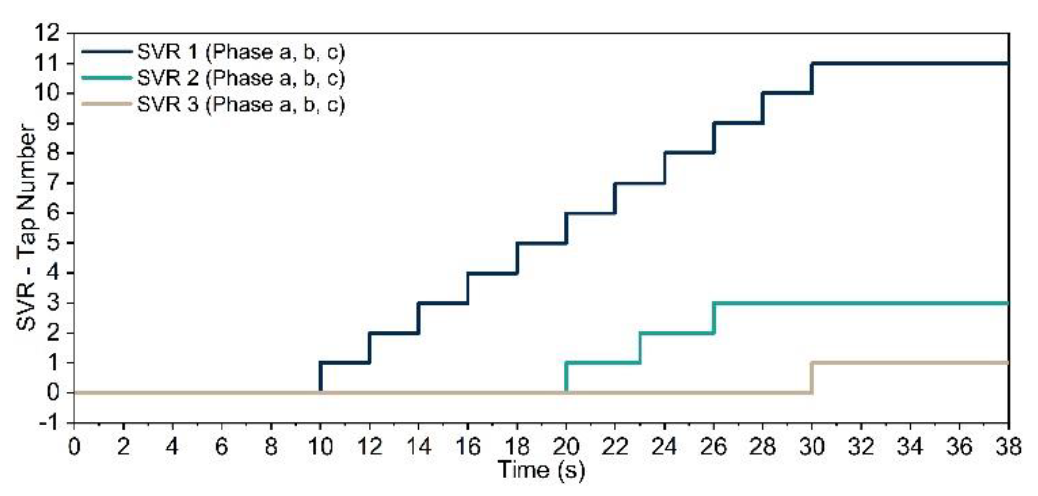
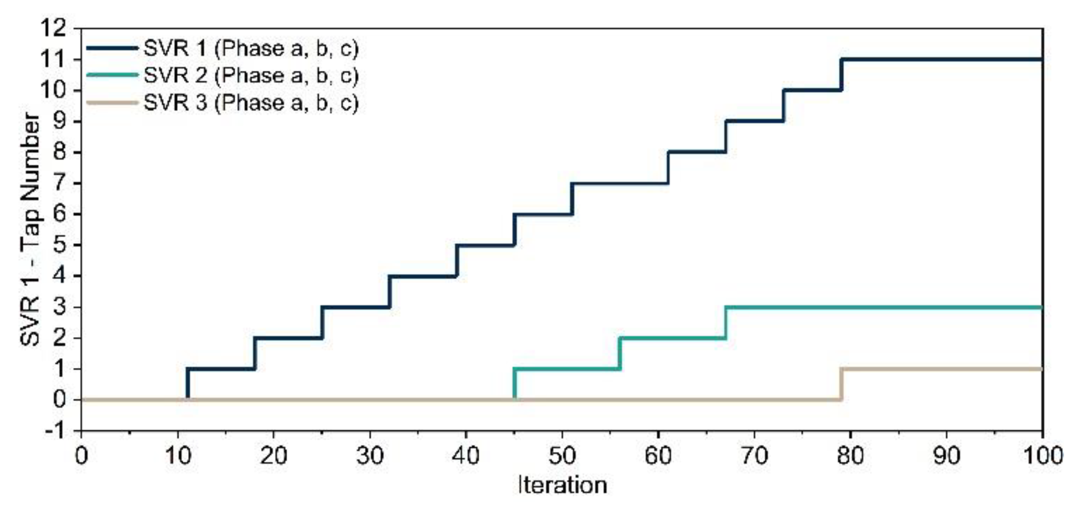
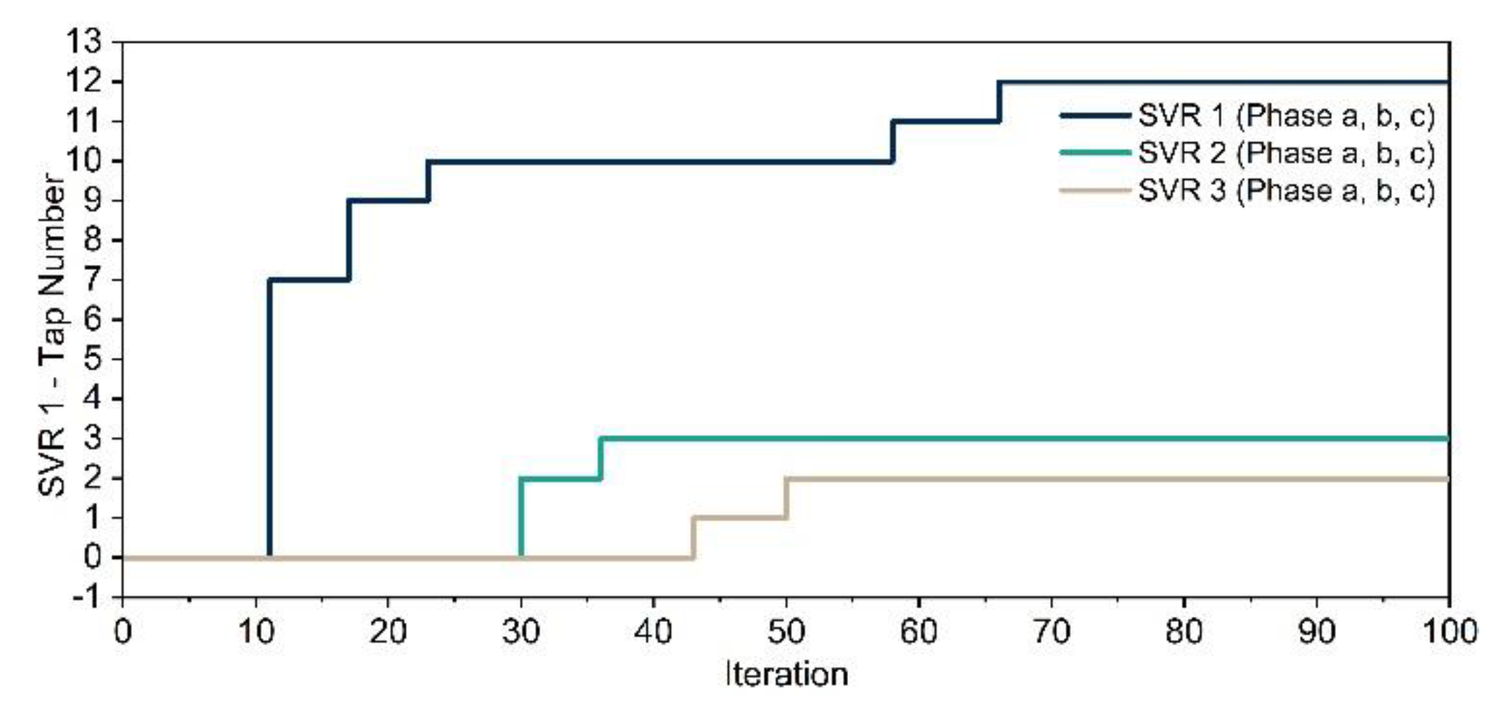
7. Validation and Performance of the Proposed Sensitivity-Based Algorithm

First and foremost, the proposed algorithm is validated against dynamic simulation in MATLAB^® Simulink using an 8-bus balanced and a 7-bus unbalanced network. In addition, the proposed approach is compared against the power flow methods of [1,3], with respect to result accuracy and convergence speed. It is noted that the method proposed in [2] presents almost identical results with the method of [1]. Therefore, the method of [2] is not simulated in this paper due to its strong similarity with [1] with respect to the produced results.

All algorithms were coded and implemented in MATLAB^®. It should be noted that for the purpose of validation against the dynamic simulation, the weather-dependent impacts were neglected in this section as traditional algorithms and Simulink do not consider weather-dependent modeling.

(A) 

8-Bus Balanced Network

Figure 3 depicts the 8-Bus network consisting of 3 SVRs and 1 DG operating in $Q\left(V\right)$ droop control mode. The $Q\left(V\right)$ droop equation is given by (15) [12,13]:

$$V_i=V_{ref\left(i\right)}-K_{q\left(i\right)}·Q_i$$

(15)

where $Q_i$, $V_{ref\left(i\right)}$, $K_{q\left(i\right)}$, $V_i$ are the positive sequence reactive power, the reference voltage, the droop gain, and the positive sequence voltage of DG i, respectively. The topology of the network is similar to the one investigated in [21]. Data about the network, the controllers of SVRs, and the DG are provided in

Table 1. Parameters of 8-Bus Network.

Length of the lines	10 km
Voltage of slack bus	7200 V
Frequency of the network	50 Hz
Resistance of lines	0.4 Ω/km
Self-reactance of the lines	0.3 Ω/km
Mutual-reactance of the lines	0.1 Ω/km
Reference voltage of SVRs	7500 V
Bandwidth of SVRs	70 V
Intentional delay of SVR1	10 s
Mechanical delay of SVR1	2 s
Intentional delay of SVR2	20 s
Mechanical delay of SVR2	3 s
Intentional delay of SVR3	30 s
Mechanical delay of SVR3	4 s
Active power of DG	1 MW
Reference voltage of DG$\left({\mathit{V}}_{\mathit{r}\mathit{e}\mathit{f}}\right)$	7500 V
Droop gain of DG$({\mathit{K}}_{\mathit{q}\left(\mathit{i}\right)} \mathit{f}\mathit{o}\mathit{r} \mathit{i}=\left\{\mathbf{1}\right\})$	$0.5 \times {10}^{-4}$ V/Var

.

The delays of the controllers are set based on their distance from the substation. The slack bus in Figure 3 is assumed to be a substation. The SVR near the substation has the fastest reaction time and as the distance from the substation increases, the reaction time increases [23,40]. All SVRs and OLTCs of the paper are considered to have, in total, 33 distinct taps (e.g., −16, …0, …+16) and can boost or reduce the voltage by ±10%. So, each tap variation changes the voltage by ±0.0625%. All SVRs are in wye configuration and are initialized to the 0 position for the purposes of simulations. Each phase of an SVR is modeled with its own local controller, which is independently controlled. The DG at bus 8 operates in $Q\left(V\right)$ mode and generates balanced phase-to-neutral voltages [14]. The network supplies four balanced three-phase loads. All the loads are modeled as constant impedance loads, as shown in

Table 2. Loads of 8-Bus Network.

Load of Buses 3, 5, 8	$Z_{La}\to R=500 \mathsf{\Omega } in parallel with X=j2000 \mathsf{\Omega }$ $Z_{Lb}\to R=500 \mathsf{\Omega } in parallel with X=j2000 \mathsf{\Omega }$ $Z_{Lc}\to R=500 \mathsf{\Omega } in parallel with X=j2000 \mathsf{\Omega }$
Load Bus 7	$Z_{La}\to R=300 \mathsf{\Omega } in parallel with X=j1200 \mathsf{\Omega }$ $Z_{Lb}\to R=300 \mathsf{\Omega } in parallel with X=j1200 \mathsf{\Omega }$ $Z_{Lc}\to R=300 \mathsf{\Omega } in parallel with X=j1200 \mathsf{\Omega }$

.

The output phase-to-neutral voltages of the three SVRs as well as the reactive power of DG are depicted in Figure 4. It should be noted that since all the loads are balanced, the three phases of the SVRs have equal voltages and undergo similar tap changes. Initially, all the voltages are below their bandwidths, and therefore, the SVRs undertake step-up actions with the intentional and mechanical delay. Initially, due to the low voltage at bus 8, the DG generates reactive power. As long as the SVRs boost their voltage, the reactive power of DG is reduced based on the droop curve (Equation (15)). The voltage of all SVRs is stabilized inside the bandwidth after 30 s. After the stabilization of SVRs, an overvoltage occurs in bus 8 due to the active power generation of DG, and thus, the DG consumes reactive power according to Equation (15).

The tap positions and switching sequence for all SVRs of the 8-bus network obtained via the dynamic simulation of Simulink are presented in Figure 5. SVR 1 executes the first switching action after an intentional time delay (10 s), followed by subsequent switching actions with a mechanical time delay (2 s), until the voltage lies within the bandwidth. Similarly, for SVR 2 and 3. Since SVR 1 has the lowest intentional and mechanical delay, it undergoes the highest number of tap changes. The final tap positions obtained via dynamic simulation for SVR 1, SVR 2 and SVR 3 is 11, 3, and 1, respectively.

In Figure 6, Figure 7, Figure 8 and Figure 9, the results of the SVR tap change versus iteration number are presented for the proposed algorithm as well as for the algorithms of [1,3]. Figure 6 presents the tap change profile of all the SVRs versus the iteration number for the proposed algorithm without consideration of sensitivity parameters (refer to Section 4). In Figure 7, the tap change profile versus iteration number is presented for the proposed algorithm with the consideration of the sensitivity parameters (refer to Section 6). The proposed algorithm, for both with and without sensitivity parameter, considers the actual reaction delays of LVCs. However, as observed in Figure 7, the consideration of sensitivity parameters yields accelerated convergence. It is reminded that the proposed algorithm, both with and without sensitivity parameters, considers the same switching algorithm, thus, it presents identical results in both cases. Their main difference is that the usage of sensitivity parameters makes the execution of a complete power flow after each switching action unnecessary, reducing the total iteration number required for the final power flow solution.

It is observed that the proposed power flow algorithm yields correct final tap positions when compared to the dynamic simulation, both with and without sensitivities. This is due to the consideration of the actual switching sequence of LVCs, as presented in Section 4. On the other hand, the LVC’s states estimated by the power flow algorithms of [1,3] do not conform to the dynamic simulation, as shown in Figure 8 and Figure 9.

Algorithm [1] is only able to correctly estimate the final tap position of SVR 2 as shown in Figure 8. It is reminded that the authors in [1] divide the LVCs into delay groups based on their reaction delays. In this example, SVR 1, SVR 2 and SVR 3 belong to the first, second and third delay group, respectively. Initially, the SVR of the first delay group reacts, by varying its taps until its voltage lies inside the bandwidth. Subsequently, the SVR of the second delay group undertakes switching actions, and so on until all SVR voltages lie inside their bandwidths. However, this process does not outline exactly the actual sequence of switching of LVCs, because in real distribution networks, the LVCs are not separated into delay groups and their reaction is not executed in the way that the algorithm of [1] describes. For instance, in the examined 8-bus network, the actual switching sequence is depicted in Figure 5 using the dynamic simulation of Simulink, which is quite different than the switching sequence predicted in [1].

The algorithm of [3] reaches final tap position in only a few iterations (Figure 9), because the algorithm updates all the LVC states simultaneously, and thus, reduces the total power flow iterations. It is reminded that algorithm [3] neglects completely the switching delays of LVCs, and updates the control variables of LVCs (e.g., taps of SVRs/OLTCs and reactive power of DGs) simultaneously, using sensitivity parameters. Due to the discrete nature of taps, after the convergence of the power flow, algorithm [1] rounds the taps to the nearest tap position.

The final voltages of the network for the investigated methods and Simulink are provided in

Table 3. Voltage profile of the investigated methods for the 8-Bus balanced network.

	Node 2a (V)	Node 3a (V)	Node 4a (V)	Node 5a (V)	Node 6a (V)	Node 7a (V)	Node 8a (V)
Simulink	6988.3309	7468.7787	7340.1399	7477.7693	7421.3890	7467.8162	7527.2533
Without sensitivity	6988.3417	7468.7902	7340.1411	7477.7687	7421.3933	7467.7770	7527.1493
With sensitivity	6988.3417	7468.7902	7340.1411	7477.7687	7421.3933	7467.7770	7527.1493
Algorithm [1]	6963.9601	7486.2571	7337.4348	7475.0117	7400.0861	7492.5872	7535.7599
Algorithm [3]	6951.5222	7472.8864	7313.0733	7495.9002	7412.0259	7504.6762	7539.9454

at the end of the paper. The proposed approach with and without sensitivities present almost identical results with those of Simulink, in contrast to the methods of [1,3] that show significant deviations.

In Figure 10, the total three-phase reactive power of the DG connected at bus 8 is presented. It operates in inductive mode according to droop Equation (15), to mitigate the voltage rise caused by the high amount of generated active power [14]. It is observed that the proposed algorithm indicates a consumption of 542 kVar, which is exactly the same as in the dynamic simulation. References [1,3] yield different results. The deviation of the reactive power in algorithms [1,3] is caused due to the inaccurate state estimation of SVRs, which inevitably leads to an imprecise reactive power calculation.

(B) 

7-Bus Unbalanced Network

An unbalanced 7-bus network consisting of an OLTC, a voltage-controlled capacitor, an SVR, and a DG is considered for further simulation and validation, as shown in Figure 11. This network was selected for simulation since it includes all kinds of LVCs (OLTC, SVR, Capacitor, DG), it is unbalanced and also its simple topology facilitates the comparison and interpretation of the simulation results. Moreover, its small size allows the execution of simulations in the time domain environment of MATLAB^® Simulink.

The DG operates in $Q\left(V\right)$ droop control mode (see Equation (15)). Data about the network, the controller of OLTC, SVR, capacitors and DG are presented in

Table 4. Parameters of 7-Bus network.

Length of the lines	10 km
Voltage of slack bus	7200 V
Frequency of the network	50 Hz
Resistance of lines	$0.4 \mathsf{\Omega }/$km
Self-reactance of the lines	$0.3 \mathsf{\Omega }$/km
Mutual-reactance of the lines	$0.1 \mathsf{\Omega }$/km
Reference voltage of SVR and OLTC	7500 V
Bandwidth of SVR and OLTC	70 V
Reference voltage of CAP	7500 V
Capacitance of each phase	$5\times {10}^{-6}$ F
Bandwidth of Capacitors	350 V
Intentional delay of OLTC	10 s
Mechanical delay of OLTC	2 s
Intentional delay of CAP	20 s
Intentional delay of SVR	30 s
Mechanical delay of SVR	4 s
Active power of DG	1 MW
Reference voltage of DG	7500 V
Droop gain of DG$({\mathit{K}}_{\mathit{q}\left(\mathit{i}\right)} \mathit{f}\mathit{o}\mathit{r} \mathit{i}=\left\{\mathbf{1}\right\})$	$0.5\times {10}^{-4}$ V/Var

. The SVR is connected in wye configuration, while OLTC in Y_g-Y_g connection [41]. Each phase of OLTC, SVR, and capacitor has its own local controller and is independently controlled. The DG generates balanced phase-to-neutral voltages [14]. The network supplies three balanced and one unbalanced three-phase constant impedance load, as shown in

Table 5. Loads of 7-Bus network.

Load of Buses 3, 6, 7	$Z_{La}\to R=500 \mathsf{\Omega } in parallel with X=j2000 \mathsf{\Omega }$ $Z_{Lb}\to R=500 \mathsf{\Omega } in parallel with X=j2000 \mathsf{\Omega }$ $Z_{Lc}\to R=500 \mathsf{\Omega } in parallel with X=j2000 \mathsf{\Omega }$
Load Bus 4	$Z_{La}\to R=500 \mathsf{\Omega } in parallel with X=j2000 \mathsf{\Omega }$ $Z_{Lb}\to R=250 \mathsf{\Omega } in parallel with X=j1000 \mathsf{\Omega }$ $Z_{Lc}\to R=500 \mathsf{\Omega } in parallel with X=j2000 \mathsf{\Omega }$

.

Table 6. LVC’s states calculated by the investigated approaches for the 7-Bus network.

	OLTC 1 Taps (Phase a, b, c)	CAP 1 (Phase a, b, c)	SVR 1 Taps (Phase a, b, c)	DG Reactive Power
Simulink	(10, 12, 10)	(ON, ON, OFF)	(2, 4, 3)	690 kvar (inductive)
Without sensitivity	(10, 12, 10)	(ON, ON, OFF)	(2, 4, 3)	690 kvar (inductive)
With sensitivity	(10, 12, 10)	(ON, ON, OFF)	(2, 4, 3)	690 kvar (inductive)
Algorithm [1]	(11, 10, 10)	(OFF, ON, OFF)	(3, 2, 2)	666 kvar (inductive)
Algorithm [3]	(11, 11, 10)	(OFF, ON, OFF)	(3, 3, 2)	625 kvar (inductive)

summarizes the calculated LVC states of each phase in the 7-Bus network using dynamic simulation, the proposed algorithm without and with sensitivity parameters, as well as the methods of [1,3]. It is observed that the proposed algorithm presents identical results with those of Simulink, confirming its accuracy. On the other hand, the calculated states of the approaches in [1,3] deviate from those of Simulink. Moreover,

Table 7. Voltage profile (of the last three buses) of the investigated methods for the 7-Bus unbalanced network.

	Node 5a (V)	Node 5b (V)	Node 5c (V)	Node 6a (V)	Node 6b (V)	Node 6c (V)	Node 7a (V)	Node 7b (V)	Node 7c (V)
Simulink	7391.8685	7311.9286	7350.1776	7484.2669	7494.7264	7488.0011	7534.5769	7534.5769	7534.5769
Without sensitivity	7391.8480	7311.9139	7350.2046	7484.2461	7494.7117	7488.0209	7534.5095	7534.5095	7534.5095
With sensitivity	7391.8480	7311.9139	7350.2046	7484.2461	7494.7117	7488.0209	7534.5095	7534.5095	7534.5095
Algorithm [1]	7340.9089	7412.7342	7381.0320	7478.5510	7505.3934	7473.2949	7533.3146	7533.3146	7533.3146
Algorithm [3]	7348.0466	7337.2315	7385.8412	7485.8225	7474.8046	7478.1643	7531.2463	7531.2463	7531.2463

at the end of the manuscript depicts indicatively the voltages of each phase for the last three buses of the network for the investigated approaches. As shown, the proposed method with and without sensitivity parameter yields near identical results with those of Simulink, while the other investigated power flow methods present significant deviations.

Finally, the number of iterations required by the algorithms to converge with an accuracy of 10⁻⁴ pu are presented in

Table 8. Required iterations for the investigated approaches in the 8-Bus network.

	Without Sensitivity	With Sensitivity	Algorithm [1]	Algorithm [3]
Required iterations	74	27	61	9

and

Table 9. Required iterations for the investigated approaches in the 7-Bus network.

	Without Sensitivity	With Sensitivity	Algorithm [1]	Algorithm [3]
Required iterations	96	29	76	8

, for the 8-Bus and 7-Bus networks, respectively. As shown, the algorithm of [3] presents the fastest convergence since it calculates all LVC’s state simultaneously ignoring their reaction delays. The proposed algorithm without the sensitivity parameters has the slowest convergence due to the successive power flow executions after each switching action. The proposed method with sensitivity parameters combines the high accuracy with the fast convergence, as no other power flow method so far.

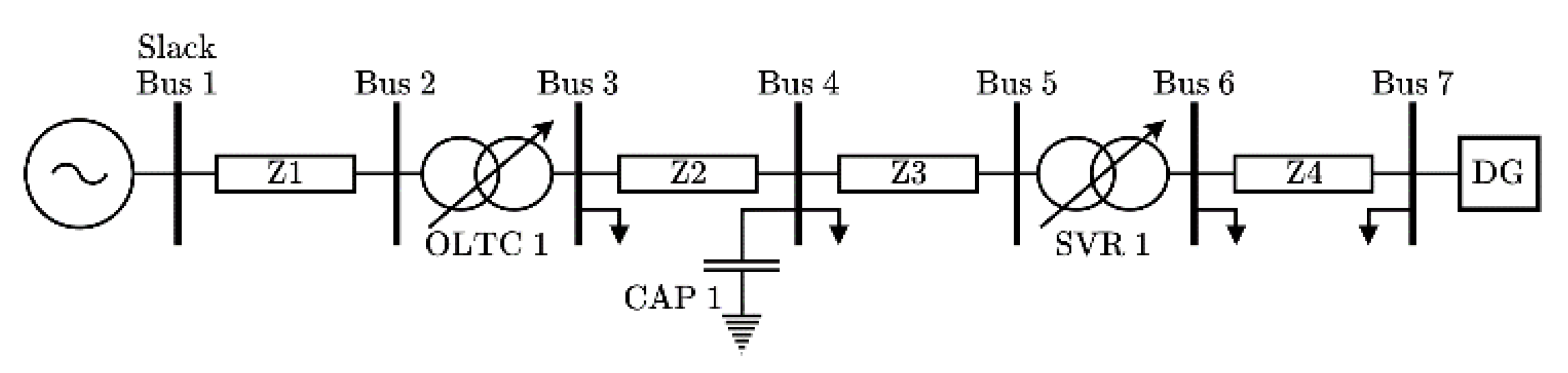
8. Influence of Weather on the LVC States and Power Flow

We conduct a case study on the large IEEE 8500-Node [42] network to compare the proposed weather-dependent algorithms (with and without sensitivities) against the conventional methods of [1,3]. Moreover, the accuracy of the proposed sensitivity-based algorithm in a large-scale network is investigated.

(A) 

Network description

Figure 12 depicts the IEEE 8500-Node Network, which has been modified by including 4 DGs operating in several modes. The network originally includes 4 SVRs and 4 capacitors [42], as shown in Figure 12.

The 4 additional DGs are connected to the buses 100, 350, 835, 1600. Data about the power profile and voltage/current profile of DGs are provided in

Table 10. DG parameters for the modified IEEE 8500-Node network.

DG #	Power Profile	Connecting Bus	Voltage/Current Profile
1	Constant PV	100	SG (Unbalanced voltage and current)
2	Droop Q(V)	350	Balanced Current
3	Droop Q(V)	835	Balanced Current
4	Constant PV	1600	Balanced Voltage

, while data about the reference voltages, the droop gains, the active powers, etc. are given in

Table 11. Parameters of the modified IEEE 8500-Node network.

Length of the lines	Given in [45]
Loads	Given in [45]
Voltage of slack bus	7200 V
Frequency of the network	50 Hz
Line type and data	All lines are Penguin ACSR [43]. The mutual impedance between all the lines was consider 0.1 j Ω/km.
Reference voltage of SVRs	7500 V
Bandwidth of SVRs	70 V
Intentional delay of SVR 1	15 s
Intentional delay of SVR 2	60 s
Intentional delay of SVR 3	60 s
Intentional delay of SVR 4	90 s
Mechanical delay of SVRs	2 s
Intentional delay of CAP 1	30 s
Intentional delay of CAP 2	45 s
Intentional delay of CAP 3	75 s
Intentional delay of CAP 4	75 s
Reference voltage of CAPs	7600 V
Bandwidth of CAPs	300 V
Capacitance of each phase	$2\times {10}^{-5}$ F
Active power of DGs	2 MW
Reference voltage of DGs$\left({\mathit{V}}_{\mathit{r}\mathit{e}\mathit{f}}\right)$	7500 V
Droop gain of DGs 2 & 3$\left({\mathit{K}}_{\mathit{q}}\right)$	${10}^{-4}$ V/var

. For DG 1, which is a synchronous generator (SG), the negative- and zero-sequence impedance are $Z_2=Z_0=0.2+j0.2$. DG 1 and DG 4 operate in constant voltage mode (treated as PV buses) and generate constant active power and positive-sequence voltage. DG 2 and DG 3 operate in droop control mode generating balanced currents (refer to Section 3.4 for more details about the operational modes of DGs).

Data of the LVCs are provided in Table 11. Each phase of the LVCs is independently controlled. The capacitors are voltage controlled and the SVRs are in wye configuration. The time delays of SVRs and capacitors are set based on their distance from the substation [23,40], while DGs react instantaneously. LVCs near substation have faster reaction times as shown in Table 11. Each controller regulates the voltage of the connection point of LVC and no line drop compensator or any other remote voltage control is applied.

Finally, all the lines of the network were replaced with the Penguin ACSR [43]. It is a single-layer conductor with a cross-sectional area 125.1 ${\mathrm{mm}}^2$ composed of a 6 Aluminum and 1 steel wire. Penguin is the largest single-layer ACSR conductor and can successfully withstand the full load of the network in both investigated environmental conditions, without thermal violation. This modification was necessary in order to simulate the influence of weather and magnetic effects into the power flow results. With the original lines of IEEE 8500-node network, this would not be possible since all lines consist of constant impedances with unknown conductor-specific details.

In Figure 13 and Figure 14, the resistance and self-reactance of Penguin ACSR conductor are presented, respectively, as a function of conductor temperature and current. The methodology to calculate the resistance and self-reactance of Figure 13 and Figure 14 is presented in [27]. It is observed that the resistance of Penguin ACSR is strongly related to both current and conductor temperature (conductor temperature is a function of both current and weather conditions [27]). Nevertheless, the impact of weather is significant as demonstrated in the following subsection.

The case study involves the simulation of two scenarios with two different weather conditions (summer and winter), as presented in

Table 12. Summer and winter weather conditions.

	Ambient Temperature Ta (°C)	Solar Irradiance qs (W/m2)	Wind Speed VW (km/h)
Summer	36.3	847	4.8
Winter	7.3	0	14.5

. The first one represents a typical summer day in Thessaloniki, Greece, while the second represents a typical winter night in the same region [44]. The directions of the lines were considered exactly as they are given in Figure 12, while the wind direction was considered parallel to the x-axis of Figure 12. The original network loads were considered for all buses [45].

(B) 

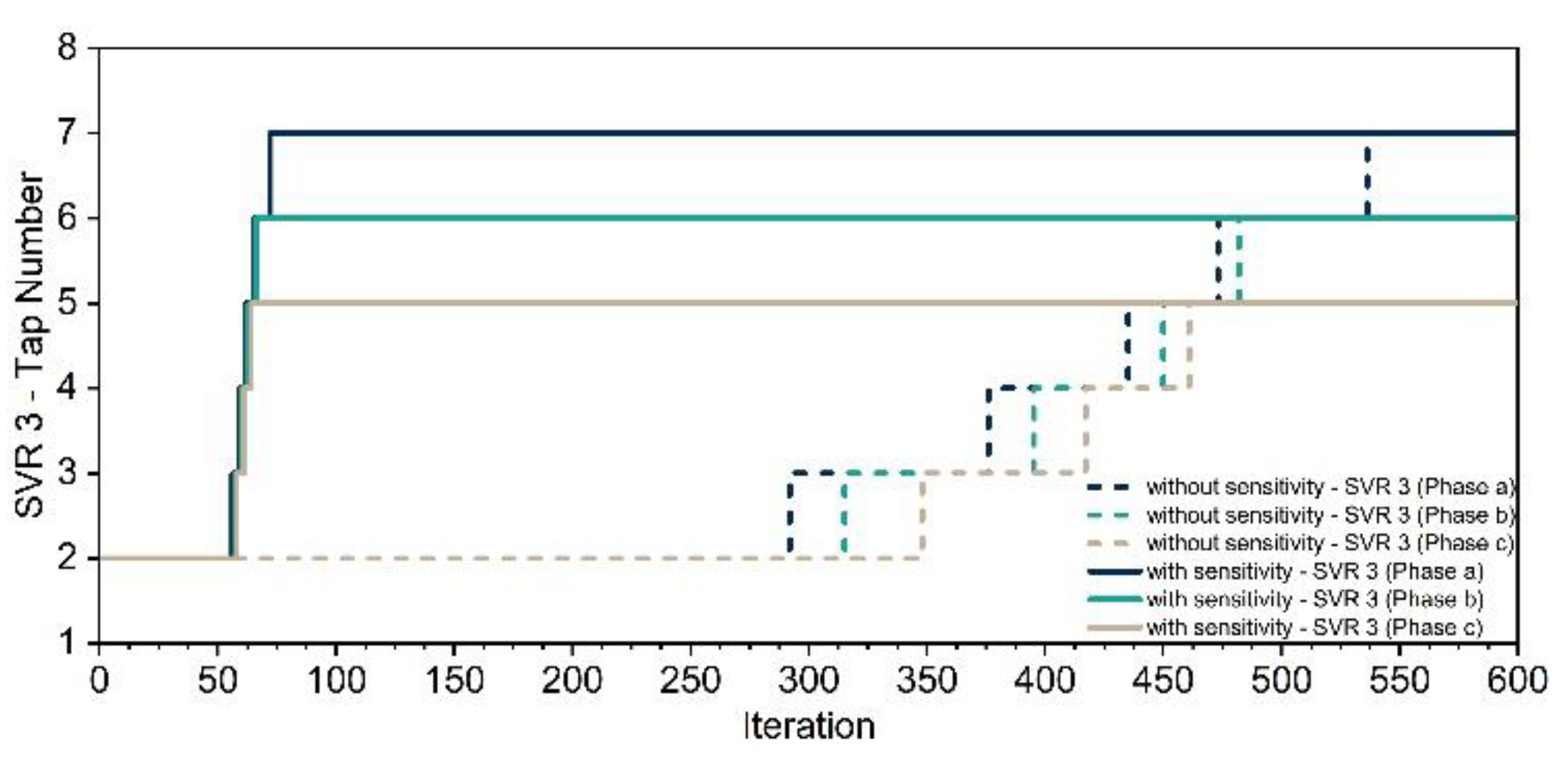
Comparison between the investigated algorithms

Simulations were executed in a generic PC with an Intel Core i7, 3.4 GHz CPU and 16 GB DDR3 RAM. As mentioned before, all investigated algorithms were coded in MATLAB^®. More specifically, the following algorithms are compared:

• Proposed weather-dependent power flow algorithm without sensitivities.
• Proposed weather-dependent power flow algorithm with sensitivities.
• Algorithm [1] with fixed impedances.
• Algorithm [3] with fixed impedances.

Usually, utilities apply traditional power flow algorithms assuming line impedances of fixed values, which are seasonally updated e.g., summer, winter to account for the weather variations. In this study, we assume fixed-line impedances for algorithm [1,3], with different values in summer and winter period, as follows:

• In Summer: $Z_{line}=0.370+0.295j \mathsf{\Omega }/\mathrm{k}$, which corresponds to a conductor current and temperature of 300 A and 60 °C, respectively, based on Figure 13 and Figure 14.
• In Winter: $Z_{line}=0.315+0.295j \mathsf{\Omega }/\mathrm{km}$, which corresponds to a conductor current and temperature of 300 A and 30 °C, respectively, based on Figure 13 and Figure 14.

Due to the large size of the network, modelling and dynamic simulations in Simulink are not possible here. In all approaches, tap position 2 was assumed as initial for all SVRs, while all the capacitors are initially considered OFF.

The tap positions and switching sequence for SVR 3 in the modified IEEE 8500-node network are presented in Figure 15. Figure 15 presents indicatively the tap positions and switching sequence for SVR 3 (all phases) obtained via the proposed algorithm, with and without the sensitivity parameters, for the summer scenario. As observed, the final tap positions are in agreement for the proposed algorithm with and without the use of sensitivity parameters. This is because both cases use similar algorithms to estimate the exact switching sequence of SVRs and capacitors (see Section 4 and Section 6). It is also observed that the use of sensitivity parameters yields a much faster solution.

A summary of the final tap positions of LVCs, for all examined algorithms, in winter and summer conditions, is presented in

Table 13. LVC’s states calculated by the investigated approaches for the modified IEEE 8500-Node.

	SVR 1 (Phase a, b, c)	SVR 2 (Phase a, b, c)	SVR 3 (Phase a, b, c)	SVR 4 (Phase a, b, c)	CAP 1 (Phase a, b, c)	CAP 2 (Phase a, b, c)	CAP 3 (Phase a, b, c)	CAP 4 (Phase a, b, c)
Proposed-Summer	(6, 6, 6)	(1, 2, 2)	(7, 6, 5)	(3, 2, 2)	(OFF, OFF, OFF)	(ON, ON, ON)	(OFF, OFF, OFF)	(ON, ON, ON)
Proposed-Winter	(6, 6, 6)	(1, 2, 2)	(6, 5, 4)	(2, 2, 2)	(OFF, OFF, OFF)	(ON, ON, ON)	(OFF, OFF, OFF)	(ON, ON, ON)
Algorithm [1]-Summer	(6, 6, 6)	(1, 2, 2)	(8, 7, 5)	(4, 3, 2)	(OFF, OFF, OFF)	(ON, ON, ON)	(OFF, OFF, OFF)	(ON, ON, ON)
Algorithm [1]-Winter	(6, 6, 6)	(1, 2, 2)	(6, 5, 5)	(3, 2, 2)	(OFF, OFF, OFF)	(ON, ON, ON)	(OFF, OFF, OFF)	(ON, ON, ON)
Algorithm [3]-Summer	(6, 6, 6)	(1, 2, 2)	(8, 7, 5)	(4, 3, 2)	(ON, ON, ON)	(ON, ON, ON)	(OFF, OFF, OFF)	(ON, ON, ON)
Algorithm [3]-Winter	(6, 6, 6)	(1, 2, 2)	(6, 5, 4)	(3, 2, 2)	(ON, ON, ON)	(ON, ON, ON)	(OFF, OFF, OFF)	(ON, ON, ON)

, while the reactive power of DGs is quoted in

Table 14. DG reactive power for the investigated approaches applied in the modified IEEE 8500-Node network.

	DG 1	DG 2	DG 3	DG 4
Proposed Algorithm (Summer)	3262 kvar (capacitive)	570 kvar (capacitive)	520 kvar (inductive)	1780 kvar (capacitive)
Proposed Algorithm (Winter)	2884 kvar (capacitive)	499 kvar (capacitive)	506 kvar (inductive)	1542 kvar (capacitive)
Algorithm [1] (summer)	3274 kvar (capacitive)	628 kvar (capacitive)	563 kvar (inductive)	1921 kvar (capacitive)
Algorithm [1] (winter)	2744 kvar (capacitive)	538 kvar (capacitive)	537 kvar (inductive)	1946 kvar (capacitive)
Algorithm [3] (summer)	3055 kvar (capacitive)	619 kvar (capacitive)	569 kvar (inductive)	1904 kvar (capacitive)
Algorithm [3] (winter)	2423 kvar (capacitive)	517 kvar (capacitive)	552 kvar (inductive)	2121 kvar (capacitive)

. As observed, for the same loading conditions, algorithms [1,3] derive different power flow results compared with the proposed approach, due to the neglect of weather and magnetic impacts as well as the actual switching sequence of LVCs. It should be noted that the proposed algorithm produces the same power flow results for the two cases, with and without sensitivity parameters. The difference observed between the two cases was in the convergence characteristics and the evolution of the solution states.

The numbers of iterations and the total computation time required by the algorithms to converge with an accuracy of 10⁻⁴ pu are presented in

Table 15. Required iterations for the investigated approaches applied in the modified IEEE 8500-Node.

	Required Iterations	Computation Time (Seconds)
Proposed-without sensitivity (summer)	553	331
Proposed-with sensitivity (summer)	79	47
Proposed-without sensitivity (winter)	261	156
Proposed-with sensitivity (winter)	49	29
Algorithm [1] (summer)	97	57
Algorithm [1] (winter)	69	40
Algorithm [3] (summer)	20	12
Algorithm [3] (winter)	14	9

, for the modified IEEE 8500-node network. As shown, the proposed algorithm with the usage of sensitivity parameters appears to be the best power flow tool for networks with LCVs, since it combines high accuracy with fast convergence and low computation time. Although algorithm [3] is by far the fastest, the results are not accurate for the aforementioned reasons.

(C) 

Accuracy of the Sensitivity-Based Algorithm

In this sub-section, we investigate how accurate the proposed sensitivity-based algorithm is, compared with the proposed algorithm without sensitivities, when applied in the large IEEE 8500-node network. Six scenarios were simulated for this purpose in the IEEE 8500-node network, explained below. In all scenarios, the winter condition was assumed for calculating the line impedances.

• Scenario 1: The loads of the network are reduced to 70% of their nominal value.
• Scenario 2: The loads of the network are increased to 120% of their nominal value.
• Scenario 3: The generated active power of each DG is increased to 3 MW.
• Scenario 4: The reference voltage of all SVRs, capacitors, and DGs is set to 7200 V.
• Scenario 5: The initial tap position for all the SVRs is set to tap number 8.
• Scenario 6: $K_{q\left(i\right)}$ for $i=\left\{1, 2, 3, 4\right\}$ is set to 1. It practically means that the DGs generate almost zero reactive power.

The results of LVC’s state are presented in

Table 16. LVC’s states calculated by the proposed method with and without sensitivities for the six Scenarios.

		SVR 1 (Phase a, b, c)	SVR 2 (Phase a, b, c)	SVR 3 (Phase a, b, c)	SVR 4 (Phase a, b, c)	CAP 1 (Phase a, b, c)	CAP 2 (Phase a, b, c)	CAP 3 (Phase a, b, c)	CAP 4 (Phase a, b, c)	Iterations
Scenario 1	without sensitivity	(6, 6, 6)	(0, 1, 1)	(3, 3, 3)	(2, 2, 2)	(OFF, OFF, OFF)	(OFF, OFF, OFF)	(OFF, OFF, OFF)	(ON, ON, ON)	143
	with sensitivity	(6, 6, 6)	(0, 1, 1)	(3, 3, 3)	(2, 2, 2)	(OFF, OFF, OFF)	(OFF, OFF, OFF)	(OFF, OFF, OFF)	(ON, ON, ON)	34
Scenario 2	without sensitivity	(7, 7, 7)	(3, 3, 2)	(14, 9, 4)	(6, 3, 2)	(OFF, OFF, OFF)	(ON, ON, ON)	(OFF, OFF, OFF)	(ON, ON, ON)	773
	with sensitivity	(7, 7, 7)	(3, 3, 2)	(14, 9, 4)	(6, 3, 2)	(OFF, OFF, OFF)	(ON, ON, ON)	(OFF, OFF, OFF)	(ON, ON, ON)	109
Scenario 3	without sensitivity	(6, 6, 6)	(0, 0, 1)	(5, 4, 3)	(2, 2, 2)	(OFF, OFF, OFF)	(OFF, OFF, OFF)	(OFF, OFF, OFF)	(ON, ON, ON)	175
	with sensitivity	(6, 6, 6)	(0, 0, 1)	(5, 4, 3)	(2, 2, 2)	(OFF, OFF, OFF)	(OFF, OFF, OFF)	(OFF, OFF, OFF)	(ON, ON, ON)	39
Scenario 4	without sensitivity	(0, 0, 0)	(1, 2, 2)	(8, 5, 4)	(4, 2, 2)	(OFF, OFF, OFF)	(OFF, OFF, OFF)	(OFF, OFF, OFF)	(ON, OFF, OFF)	169
	with sensitivity	(0, 0, 0)	(1, 2, 2)	(8, 5, 4)	(4, 2, 2)	(OFF, OFF, OFF)	(OFF, OFF, OFF)	(OFF, OFF, OFF)	(ON, OFF, OFF)	38
Scenario 5	without sensitivity	(7, 7, 7)	(1, 1, 1)	(8, 4, 2)	(3, 2, 0)	(OFF, OFF, OFF)	(ON, ON, ON)	(OFF, OFF, OFF)	(ON, ON, ON)	871
	with sensitivity	(7, 7, 7)	(1, 1, 1)	(8, 4, 2)	(3, 1, 1)	(OFF, OFF, OFF)	(ON, ON, ON)	(OFF, OFF, OFF)	(ON, ON, ON)	116
Scenario 6	without sensitivity	(6, 6, 6)	(2, 3, 3)	(9, 8, 7)	(3, 2, 2)	(ON, ON, ON)	(ON, ON, ON)	(OFF, OFF, OFF)	(ON, ON, ON)	379
	with sensitivity	(6, 6, 6)	(2, 3, 3)	(9, 8, 7)	(3, 2, 2)	(ON, ON, ON)	(ON, ON, ON)	(OFF, OFF, OFF)	(ON, ON, ON)	70

for the proposed method without and with the use of sensitivity. As shown, the algorithms produce identical results in the first four and 6th scenarios. In most of the simulations presented in this manuscript, there has been full agreement between the proposed algorithm without and with sensitivities. However, a slight difference is observed in the state estimation of SVR 4 of scenario 5 (highlighted in bold in Table 16), where the two algorithms output (3, 2, 0) and (3, 1, 1), respectively. This difference is attributed to the fact that the usage of sensitivities involves predictor and corrector steps, which are approximations. Nevertheless, this difference is negligible in comparison to the major reduction in the number of iterations required to obtain the power flow solution, when sensitivities are adopted, as observed in the last column of Table 16.

(D) 

Weather Data Acquisition

The real-time measurement of local weather parameters is feasible today since the number of automatic weather stations (AWSs) has been considerably increased worldwide [44]. For instance, in Greece, National Observatory of Athens (NOA) has installed, over the last 15 years, more than 430 automatic weather stations over Greece (see Figure 16). All weather stations record (every 10 min) the 10-min average values of wind speed, wind direction, ambient temperature and solar radiation, namely all the weather parameters required by the proposed approach. The data are provided in a real-time manner to potential users, through web-based platforms [44], and therefore, they are currently very easily accessible.

9. Conclusions

This paper presents a sensitivity-based three-phase weather-dependent power flow algorithm for simulating distribution networks with LVCs. The proposed algorithm has four distinct characteristics: (a) it considers the three-phase unbalanced nature of distribution systems, (b) the operating state of LVCs is calculated using sensitivity parameters accelerating the convergence speed of the algorithm, (c) it considers the exact switching sequence of LVCs based on their reaction time delays, and (d) the influence of weather variations on the power flow is also taken into consideration. The proposed algorithm has high accuracy and low computational complexity and is therefore can constitute an important tool in offline and real-time applications of distribution systems. The proposed approach was compared against some state-of-the-art power flow methods using a 7-bus, an 8-bus and the IEEE 8500-node network. The results indicate that the existing algorithms can produce inaccurate power flow results and LVC’s states, due to the imprecise consideration of LVC’s switching sequence. Finally, it was deduced through simulations, that for a more precise estimation of LVC’s states and power flow results, the weather variations should be considered in the power flow.

References

1. Roytelman, I.; Ganesan, V. Modeling of local controllers in distribution network applications. IEEE Trans. Power Del. 2000, 15, 1232–1237. [Google Scholar] [CrossRef]
2. Jabr, R.A.; Džafic, I.; Karaki, S. Tracking Transformer Tap Position in Real-Time Distribution Network Power Flow Applications. IEEE Trans. Smart Grid 2016, 9, 2442–2452. [Google Scholar] [CrossRef]
3. Džafic, I.; Jabr, R.A.; Halilovic, E.; Pal, B.C. A sensitivity approach to model local voltage controllers in distribution networks. IEEE Trans. Power Syst. 2014, 29, 1419–1428. [Google Scholar] [CrossRef]
4. Todescato, M.; Carli, R.; Schenato, L.; Barchi, G. Smart Grid State Estimation with PMUs Time Synchronization Errors. Energies 2020, 13, 5148. [Google Scholar] [CrossRef]
5. Garcia, P.A.; Pereira, J.L.; Carneiro, S.; Da Costa, V.M.; Martins, N. Three-phase power flow calculations using the current injection method. IEEE Trans. Power Syst. 2000, 15, 508–514. [Google Scholar] [CrossRef]
6. Junior, H.M.R.; Melo, I.D.; Nepomuceno, E.G. An interval power flow for unbalanced distribution systems based on the Three-Phase Current Injection Method. Int. J. Electr. Power Energy Syst. 2022, 139, 107921. [Google Scholar] [CrossRef]
7. Murari, K.; Padhy, N.P. Graph-theoretic based approach for the load-flow solution of three-phase distribution network in the presence of distributed generations. IET Gener. Transm. Distrib. (IET) 2020, 14, 1627–1640. [Google Scholar] [CrossRef]
8. Verma, R.; Sarkar, V. Active distribution network load flow analysis through non-repetitive FBS iterations with integrated dg and transformer modelling. IET Gener. Transm. Distrib. 2019, 13, 478–484. [Google Scholar] [CrossRef]
9. Wang, X.; Shahidehpour, M.; Jiang, C.; Tian, W.; Li, Z.; Yao, Y. Three-phase distribution power flow calculation for loop-based microgrids. IEEE Trans. Power Syst. 2018, 33, 3955–3967. [Google Scholar] [CrossRef]
10. Chang, S.K.; Brandwajn, V. Adjusted solutions in fast decoupled load flow. IEEE Trans. Power Syst. 1988, 3, 726–733. [Google Scholar] [CrossRef]
11. Joseph, A.; Smedley, K.; Mehraeen, S. Secure High DER Penetration Power Distribution via Autonomously Coordinated Volt/VAR Control. IEEE Trans. Power Deliv. 2020, 35, 2272–2284. [Google Scholar] [CrossRef]
12. Std 1547-2018; IEEE Standard for Interconnection and Interoperability of Distributed Energy Resources with Associated Electric Power Systems Interfaces. IEEE: New York, NY, USA, 2018.
13. Kraiczy, M.; Stetz, T.; Braun, M. Parallel Operation of Transformers with on Load Tap Changer and Photovoltaic Systems with Reactive Power Control. IEEE Trans. Smart Grid 2018, 9, 6419–6428. [Google Scholar] [CrossRef]
14. Pompodakis, E.E.; Kryonidis, G.; Demoulias, C.; Alexiadis, M. A Generic Power Flow Algorithm for Unbalanced Islanded Hybrid AC/DC Microgrids. IEEE Trans. Power Syst. 2021, 36, 1107–1120. [Google Scholar] [CrossRef]
15. Peterson, N.M.; Meyer, W.S. Automatic adjustment of transformer and phase shifter taps in the Newton power flow. IEEE Trans. Power App. Syst. 1971, PAS-90, 103–108. [Google Scholar] [CrossRef]
16. Cetindag, B.; Kocar, I.; Guèye, A.; Karaagac, U. Modeling of Step Voltage Regulators in Multiphase Load Flow Solution of Distribution Systems Using Newton’s Method and Augmented Nodal Analysis. Elect. Power Comp. Syst. 2017, 45, 1667–1677. [Google Scholar] [CrossRef]
17. Expósito, A.G.; Ramos, E.R.; Džafic, I. Hybrid real–complex current injection-based load flow formulation. Elect. Power Syst. Res. 2015, 119, 237–246. [Google Scholar] [CrossRef]
18. Kocar, I.; Mahseredjian, J.; Karaagac, U.; Soykan, G.; Saad, O. Multiphase load-flow solution for large-scale distribution systems using MANA. IEEE Trans. Power Deliv. 2014, 29, 908–915. [Google Scholar] [CrossRef]
19. Viawan, F.A.; Karlsson, D. Combined local and remote voltage and reactive power control in the presence of induction machine distributed generation. IEEE Trans. Power Syst. 2007, 22, 2003–2012. [Google Scholar] [CrossRef]
20. Viawan, F.A.; Karlsson, D. Voltage and reactive power control in systems with synchronous machine-based distributed generation. IEEE Trans. Power Del. 2008, 23, 1079–1087. [Google Scholar] [CrossRef]
21. Yorino, N.; Zoka, Y.; Watanabe, M.; Kurushima, T. An optimal autonomous decentralized control method for voltage control devices by using a multi-agent system. IEEE Trans. Power Syst. 2015, 30, 2225–2233. [Google Scholar] [CrossRef]
22. Ranamuka, D.; Agalgaonkar, A.P.; Muttaqi, K.M. Examining the interactions between DG units and voltage regulating devices for effective voltage control in distribution systems. IEEE Trans. Ind. Appl. 2017, 33, 1485–1496. [Google Scholar] [CrossRef]
23. Ranamuka, D.; Agalgaonkar, A.; Muttaqi, K. Online voltage control in distribution systems with multiple voltage regulating devices. IEEE Trans. Sustain. Energy 2014, 5, 617–628. [Google Scholar] [CrossRef]
24. Valverde, G.; Cutsem, T.V. Model predictive control of voltages in active distribution networks. IEEE Trans. Smart Grid 2013, 4, 2152–2161. [Google Scholar] [CrossRef] [Green Version]
25. El Moursi, M.S.; Zeineldin, H.H.; Kirtley, J.L.; Alobeidli, K. A dynamic master/slave reactive power-management scheme for smart grids with distributed generation. IEEE Trans. Power Deliv. 2014, 29, 1157–1167. [Google Scholar] [CrossRef]
26. Agalgaonkar, Y.; Pal, B.; Jabr, R. Distribution voltage control considering the impact of PV generation on tap changers and autonomous regulators. IEEE Trans. Power Syst. 2014, 29, 182–192. [Google Scholar] [CrossRef] [Green Version]
27. Pompodakis, E.; Ahmed, A.; Alexiadis, M. A Three-Phase Weather-Dependent Power Flow Approach for 4-Wire Multi-Grounded Unbalanced Microgrids with Bare Overhead Conductors. IEEE Trans. Power Syst. 2021, 36, 2293–2303. [Google Scholar] [CrossRef]
28. Ahmed, A.; McFadden, F.J.S.; Rayudu, R. Weather-Dependent Power Flow Algorithm for Accurate Power System Analysis Under Variable Weather Conditions. IEEE Trans. Power Syst. 2019, 34, 2719–2729. [Google Scholar] [CrossRef]
29. Hsieh, T.-Y.; Chen, T.-H.; Yang, N.-C. Matrix decompositions-based approach to Z-bus matrix building process for radial distribution systems. Int. J. Electr. Power Energy Syst. 2017, 89, 62–68. [Google Scholar] [CrossRef]
30. Std 738-2012 (Revision of IEEE Std 738-2006-Incorporates IEEE Std 738-2012 Cor 1-2013); IEEE Standard for Calculating the Current-Temperature Relationship of Bare Overhead Conductors. IEEE: New York, NY, USA, 2013; pp. 1–72.
31. ACL Cables. Online Catalog. Available online: http://www.acl.lk/front_img/1502964374ACL_bare_conductor_2015(2).pdf (accessed on 7 October 2020).
32. Roytelman, I.; Ganesan, V. Coordinated local and centralized control in distribution management systems. IEEE Tans. Power Deliv. 2000, 15, 718–724. [Google Scholar] [CrossRef]
33. Pompodakis, E.E.; Kryonidis, G.C.; Alexiadis, M.C. A comprehensive three-phase step voltage regulator model with efficient implementation in the Z-bus power flow. Electr. Power Syst. Res. 2021, 199, 107443. [Google Scholar] [CrossRef]
34. Pompodakis, E.E.; Kryonidis, G.C.; Alexiadis, M.C. OLTC transformer model connecting 3-wire MV with 4-wire multigrounded LV networks. Electr. Power Syst. Res. 2021, 192, 107003. [Google Scholar] [CrossRef]
35. Eaton Cooper Power Series, Voltage Regulators vs. Load Tap Changers. Voltage Regulators Reference Data TD225012EN. 2017. Available online: https://www.eaton.com/content/dam/eaton/products/medium-voltage-power-distribution-control-systems/voltage-regulators/voltage-regulators-vs-load-tap-changers-information-td225012en.pdf (accessed on 2 March 2022).
36. Bettanin, A.; Coppo, M.; Savio, A.; Turri, R. Voltage management strategies for low voltage networks supplied through phase-decoupled on-load-tap-changer transformers. In Proceedings of the 2017 AEIT International Annual Conference, Cagliari, Italy, 20–22 September 2017; pp. 1–6. [Google Scholar]
37. Fundamentals Ltd Power Systems Technology. Enhanced Voltage Control EAVC Settings Calculation Guide. Fundamentals Reference F9183. 15 August 2018. Available online: https://www.enwl.co.uk/globalassets/innovation/enwl011/enwl011-closedown-appendix-d.pdf (accessed on 2 March 2022).
38. Pompodakis, E.; Ahmed, A.; Alexiadis, M. A Sensitivity-Based Three-Phase Weather-Dependent Power Flow Algorithm for Networks with Local Controllers—Supplementary. TechRxiv 2020. preprint. [Google Scholar] [CrossRef]
39. Pompodakis, E.; Chrysochos, A.I.; Ahmed, A.; Alexiadis, M.C. Time-Series Temperature-Dependent Power Flow Considering Unbalanced Thermoelectric Equivalent Circuits for Underground LV and MV Cables. TechRxiv 2021. preprint. [Google Scholar] [CrossRef]
40. Don Wareham, Step Voltage Regulators. Cooper Power Systems by Eaton. 2013. Available online: http://www.cscos.com/wp-content/uploads/NY1839-Eaton-Regulators-D.Wareham.pdf (accessed on 1 November 2020).
41. Huseinagić, I.; Džafić, I.; Jabr, R.A. A compensation technique for unsymmetrical three-phase power flow. In Proceedings of the International Symposium on Industrial Electronics (INDEL), Banja Luka, Bosnia, 3–5 November 2016. [Google Scholar]
42. Arritt, R.F.; Dugan, R.C. The IEEE 8500-node test feeder. In Proceedings of the IEEE PES T&D 2010, New Orleans, LA, USA, 19–22 April 2010; pp. 1–6. [Google Scholar]
43. DICABS Conductors Technical Catalogue. Online Catalog. Available online: https://www.academia.edu/34442747/Conductor_Technical_Catalogure (accessed on 25 February 2020).
44. Lagouvardos, K.; Kotroni, V.; Bezes, A.; Koletsis, I.; Kopania, T.; Lykoudis, S.; Mazarakis, N.; Papagiannaki, K.; Vougioukas, S. The automatic weather stations NOANN network of the National Observatory of Athens: Operation and database. Geosci. Data J. 2017, 4, 4–16. [Google Scholar] [CrossRef]
45. IEEE PES. Distribution Test Feeders, “8500-Node Test Feeder”. Available online: http://www.ewh.ieee.org/soc/pes/dsacom/testfeeders/index.html (accessed on 2 March 2022).
Figure 1. A simplified network including a three-phase SVR, capacitor, DG, OLTC. All control variables are included in the current sources.
Energies 15 01977 g001
Figure 2. Flowchart of the proposed sensitivity-based power flow method.
Energies 15 01977 g002
Figure 3. 8-Bus network consisting of 3 SVRs and 1 DG.
Energies 15 01977 g003
Figure 4. Phase to neutral voltage at the outputs of SVRs (left vertical axis) and reactive power of DG (right vertical axis).
Energies 15 01977 g004
Figure 5. Switching sequence of SVRs in the 8-Bus network versus time as calculated by MATLAB® Simulink.
Energies 15 01977 g005
Figure 6. Switching sequence of the three SVRs for the 8-Bus network versus iteration number, as calculated by the proposed method without sensitivity.
Energies 15 01977 g006
Figure 7. Switching sequence of the three SVRs for the 8-Bus network versus iteration number, as calculated by the proposed method with sensitivity.
Energies 15 01977 g007
Figure 8. Switching sequence of the three SVRs for the 8-Bus network versus iteration number, as calculated by the algorithm of reference [1].
Energies 15 01977 g008
Figure 9. Switching sequence of the three SVRs for the 8-Bus network versus iteration number, as calculated by the algorithm of reference [3].
Energies 15 01977 g009
Figure 10. Total reactive power consumption of the DG at bus 8.
Energies 15 01977 g010
Figure 11. 7-Bus unbalanced network consisting of one OLTC, one SVR, one three-phase capacitor and one DG.
Energies 15 01977 g011
Figure 12. IEEE 8500-Node network consisting of 4 SVRs and 4 three-phase capacitors [42].
Energies 15 01977 g012
Figure 13. Resistance of Penguin ACSR conductor, as a function of conductor temperature and current, considering weather and magnetic impacts.
Energies 15 01977 g013
Figure 14. Self-Reactance of Penguin ACSR conductor, as a function of conductor temperature and current, considering weather and magnetic impacts.
Energies 15 01977 g014
Figure 15. Switching sequence of SVR 3 in the modified IEEE 8500-node network for summer obtained via the proposed algorithm.
Energies 15 01977 g015
Figure 16. Geographical distribution of the network of automatic weather stations over Greece [44]. The red points indicate the position of weather stations.
Energies 15 01977 g016