Investigating Energy Use in a City District in Nordic Climate Using Energy Signature

Abstract

This paper focuses on multi-family buildings in a Swedish city district, erected between 1965 and 1973, which are now in need of renovation. For the two types of multi-family buildings in the district, tower buildings and low-rise buildings, dynamic energy use is predicted by using an energy signature method. The energy signature is then used to calculate the primary energy use number of the building stock, according to calculations methods dictated by Swedish building regulations. These regulations are also used to assess which multi-family buildings are in need of renovation, based on the buildings’ primary energy use. For buildings that need energy renovations, it is simulated so that the energy use of each multi-family building complies with these same building regulations. The proposed methodology for simulating energy renovation also determines new energy signature parameters, related to building heat loss coefficient, balance temperature and domestic hot water usage. The effects of simulated renovation are displayed in a duration diagram, revealing how a large-scale renovation affects the district’s heat load in different annual periods, which affects the local district heating system. Sensitivity analysis is also performed before and after simulated energy renovation.

1. Introduction

The annual rate of energy renovation in the European Union is currently only about 1%, which is too slow to meet the goals of reducing energy use and greenhouse gas emissions [1]. In order to increase this renovation rate, the Energy Performance of Buildings Directive has been adopted [2]. Among other things, this directive requires that union member states set minimum energy performance requirements for new and renovated buildings, and that all new buildings must be nearly zero-energy buildings (NZEBs). Additionally, energy renovation of existing buildings to NZEB standard should be encouraged [3].

Between 1964 and 1975, over one million housing units were built in Sweden, in what is called the Million Homes Programme [4]. Million Homes Programme buildings include both single-family and multi-family buildings, where the latter constituted two-thirds of constructed housing units [5]. In many cases they were built in a very similar style using similar construction technologies, and were clustered together in, at the time, new city districts. Since the Million Homes Programme buildings are now more than 50 years old, many are in need of renovation.

To study large buildings stocks (such as Sweden’s Million Homes Programme buildings), it is common to use categorisation based on physical properties of the building stock [6,7,8]. After categorisation, the building stock is modelled as representative buildings, chosen from each category, or as archetype buildings, based on average properties from each category [9,10,11]. These representative or archetype buildings are then scaled up to the entire building stock at district, city, regional or national level. Renovation of representative buildings can then be used to investigate renovation of building stocks.

Modelling a representative building may be done with either a physical or statistical method. Disadvantages of using physical, also called law-driven, methods include that they require a large amount of information about the building or building stock, such as the building’s thermal properties [12] and are computer intensive [13]. The physical methods also require model build-up and validation, and on-site inspections and monitoring should be performed [14].

Some advantages of physical methods are that they enable evaluation of new technologies, such as solar energy [13]. Physical methods are capable of predicting energy use for non-existent buildings, which may be built in the future [15]. It is also possible to study individual energy efficiency measures, such as additional external wall insulation [16].

The other way to model buildings and building categories is to use a purely statistical, data-driven method. Statistical methods have several advantages, the main one being that the actual behaviour of the buildings is modelled [17,18]. There is a growing body of data collected from buildings and their operation [13,19,20] and these methods are relatively simple to implement [21,22]. However, some of the advantages of physical methods are conversely disadvantages with statistical methods. It is not possible to study individual energy efficiency measures with statistical methods. Additionally, they are dependent on historical building data, and thus cannot be used for non-existent buildings.

Statistical data on, e.g., thermal energy use, has been used for a number of purposes: to develop archetypes [23], cluster residential buildings [24,25] and to simulate and evaluate large-scale city models [26,27]. In addition to using a purely physical or statistical model, it is possible to use a hybrid method, as done by Martinez-Soto and Jentsch [28]. Statistical models, physical methods and GIS data can also be combined to model building energy use [29].

One type of statistical method is the regression-based energy signature (ES) method. ES has been used to describe the energy use of individual buildings, for both single-family and multi-family buildings [17,19,30], as well as building stocks. Aydinalp-Koksal and Ugursal [21] used a regression-based method to study the energy use of the Canadian residential building stock and found that it had good agreement to both actual values and when compared to other methods. Mastrucci et al. [22] used multiple linear regression to estimate the natural gas and electricity consumption in a city containing 300,000 housing units, and found that the methods yielded results that were accurate and statistically significant. Despite these examples, the majority of papers on energy use on the district or community level use physical rather than statistical methods [31].

Many ES methods are linear models, which on building level can give information on building envelope, balance temperature and base load. However, it is also possible to use a non-linear ES method, as suggested in [32]. ES methods are often applied in cold climates, where the method describes the heating requirement of buildings, which is especially important in Nordic countries. ES can also be used in warmer climates, where space cooling dominates energy use [33,34,35].

In addition to the applications of ES and other statistical (data-driven) methods that have been reported above, Yang et al. [36] stated in their review that future data-driven models can be an effective way of investigating energy renovation potential. The authors also wrote that applications of data-driven compared to physical (law-driven) methods have to date been limited, due to later availability of measured building data, that can be used for data-driven methods. Furthermore, data-driven methods have been stated as a way to support the building sector towards NZEB standard and further decarbonisation, through investigation of renovation schemes [37,38,39]. Examples of data-driven methods to estimate energy renovation can be found, though the number of applications is relatively low and these are commonly supported by other tools such as physical methods, GIS-data or categorisation [22,29,35,40]. The more frequent uses of data-driven methods are to investigate current energy use, for small or large-scale analysis [41,42,43]. Deb and Schlueter [44] also stated that there are no studies available that exclusively use machine-learnings methods and measured building data, to estimate energy renovation. Although the number is low, there seems to be studies that exclusively use data-driven methods and measured building data, for estimation of energy renovation [45,46,47].

The purpose of the present work is to use a statistical procedure, i.e., ES method, based on hourly heating supply and temperature data, as a cost and time effective method to predict the thermal performance of residential buildings in a Swedish city district, before and after simulated energy renovation. The novelty of the work lies in using the ES method to investigate thermal performance status and how the method is used to simulate energy renovation on 95 multi-family buildings in the studied district, which as shown above, is lacking in the literature. The purpose is also to show how this method and the findings can be useful to building owners and energy providers. In addition to investigating energy use of the district, the method is used to address effects of simulated renovation on the local district heating (DH) system.

2. Description of the Multi-Family Building Stock and the District Heating System

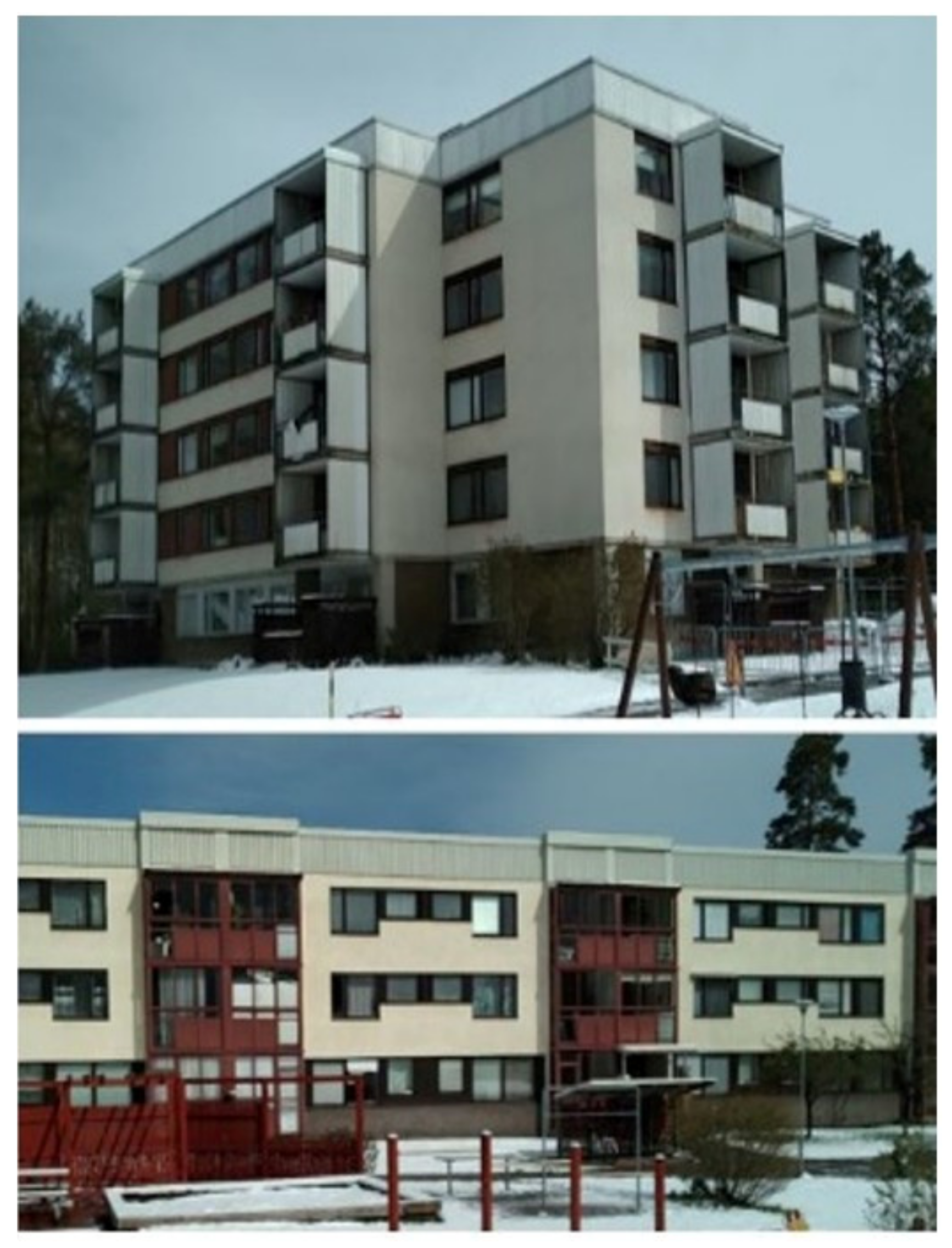
The studied district is Sätra in the city of Gävle, 170 km north of Stockholm, Sweden. The district’s multi-family building stock encompasses two types: five-story tower buildings and low-rise buildings with two or three stories, all built within the abovementioned Million Homes Programme period. When newly built, all multi-family buildings in the district had similar thermal performance, since they used similar blueprints, and were built to fulfil the same building regulations. The buildings were all constructed using aerated concrete and concrete walls, with white rendered facades. Ground floor level walls were made of concrete, while the rest of the floors were made of aerated concrete. Ventilation systems are exhaust-only, with exhaust diffusers in kitchens and bathrooms. None of the buildings contain space cooling, neither before nor after renovation.

Since the early 2000s, the district has been subjected to several renewal projects [48]. Among other things, some of the multi-family buildings in the district have undergone deep energy renovation. Renovation consisted of adding insulation to external walls, ground floor and roof, changing the ventilation system and replacing windows and doors. These measures reduced their energy use by almost 50%. However, due to different owners over time and with different ambitions in terms of energy use target, different renovations have been implemented across the district. Since 2011, the Sätra district has been labelled as a cultural heritage environment of national interest status, restricting changes to building exteriors. This status has increased the costs of technical solutions and renovation [49].

The main differences between the building types in the district, tower buildings and low-rise buildings, are their ground floor area and form factors (envelope area/volume). Form factors for tower buildings are roughly 0.33 and for low-rise buildings 0.49. Figure 1 shows examples of the building types in the studied district, illustrating these differences.

In total, there are 95 multi-family buildings: 60 tower buildings and 35 two- and three-story low-rise buildings. The tower buildings are all five-story buildings, having total heated floor area ranging from roughly 2000–2800 m². The difference in size depends on whether the tower buildings contain a laundry room, basement, and various storage and technical rooms. The laundry, storage and technical rooms in the tower buildings are either in the basement or ground floor. The low-rise buildings’ heated floor areas differ between roughly 700–5500 m², depending on the number of entrances, and consequently the number of flats. Total heated floor area in the district is approximately 145,200 m² and 74,500 m² for tower and low-rise buildings, respectively.

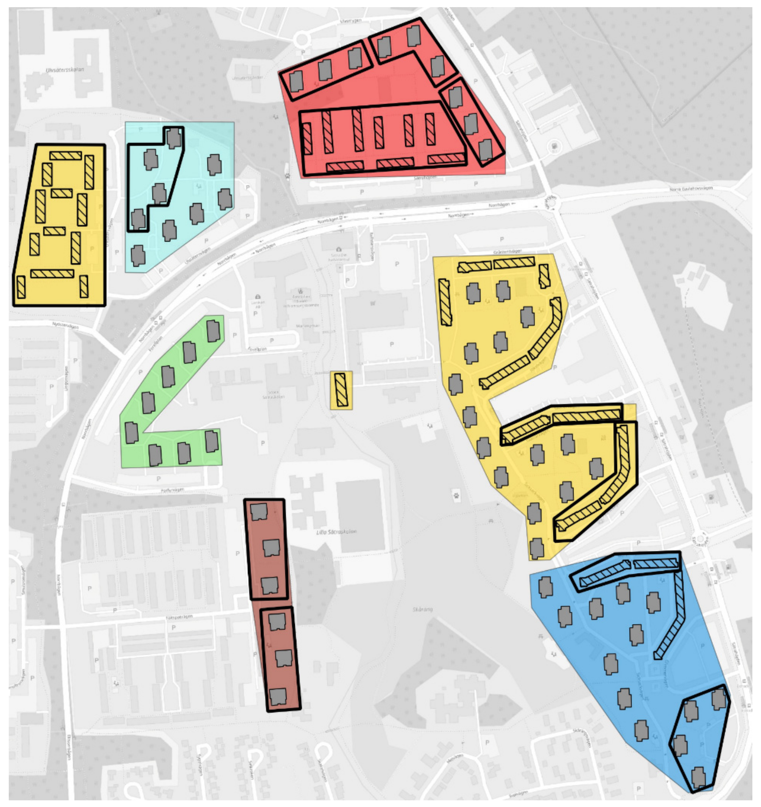
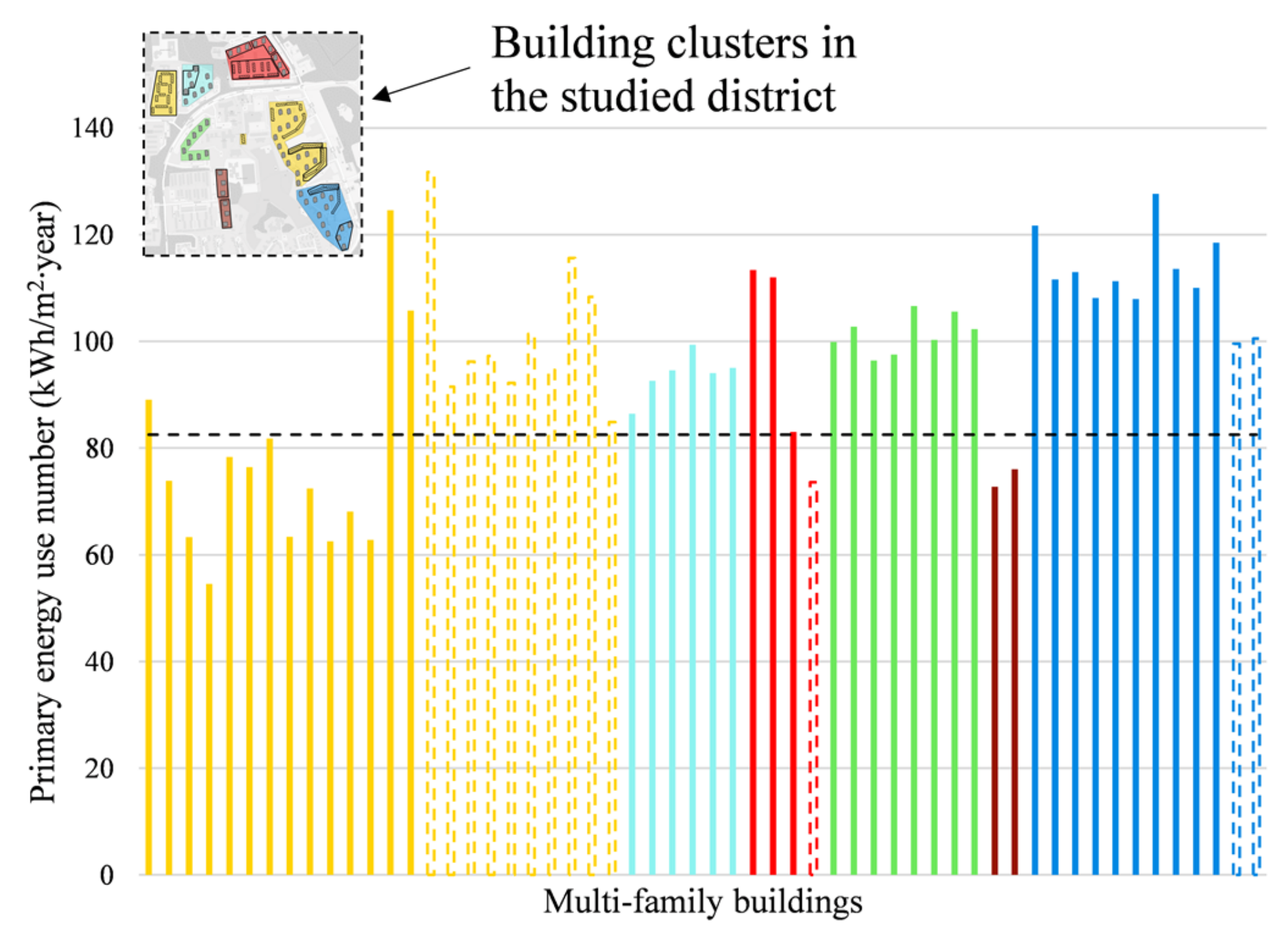
Figure 2 shows the part of the Sätra district that contains multi-family buildings, where grey squares signify tower buildings and elongated striped structures signify low-rise buildings. Background colours in Figure 2 display clusters of property owners’ building stocks. The clusters marked in red and dark red are the district’s two housing cooperatives (condominiums). The other four property owners are all rental companies. One of these rental companies is the municipal public building owner in the city of Gävle (marked in yellow), and the other five property owners are all private companies. Some buildings share the same DH substation, which has been marked with a black encircling outline. All others have their own DH substation. The DH substations also serve as measuring point for supplied DH. This means that although the district contains 95 multi-family buildings, the number of measurement points is only 56. Buildings not marked in Figure 2 are single-family buildings, a supermarket, restaurants, etc., which are omitted in the present study.

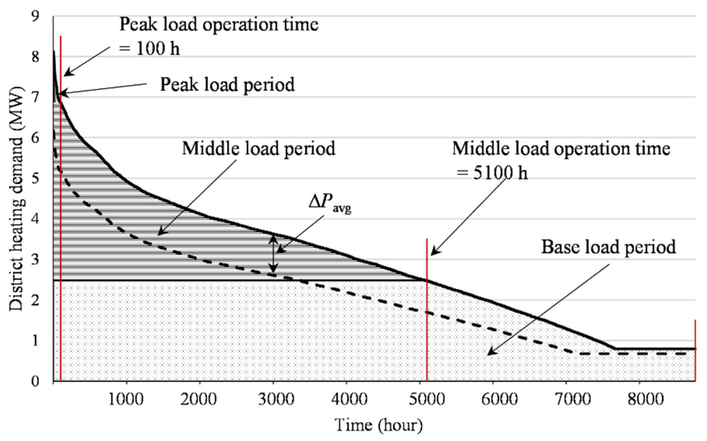
Multi-family buildings in the district are all heated by DH, supplied by the local company Gävle Energi AB. Except for one tower building, supplied DH data was available for all buildings, starting from either 2013, 2016 or 2017. The heat supply sources to Gävle Energi AB’s DH system are mainly categorized by production and cost strategies [50]. The production is divided as periods of Peak load, Middle load and Base load. Peak load plant is oil heat-only boiler with an operation time of 0–100 h. Middle load plants are biofuel combined heat and power (CHP) plants and condenser heat from industrial biofuel CHP plant with a duration time of 0–5100 h. Base load plants are evaporator heat, flue gas condensation heat and excess heat from nearby industry with a duration time of 0–8760 h. This information has been derived from a database on information from Gävle Energi AB (2012/2013).

3. Methods

The Methods section is structured as follows. Section 3.1 contains a brief explanation of the ES method as well as its required input data. Section 3.2 explains how the ES method is used to predict district level energy use in two different ways. Section 3.3 contains sub-sections explaining the primary energy use number and how it is used in this paper. Finally, Section 3.4 explains which factors were subjected to sensitivity analysis. In equations in the Methods section, E symbolizes annual energy use, in kWh or kWh/m², while P symbolizes demand in kW.

3.1. Description and Inputs for the Energy Signature Method

The ES method was developed and validated for a tower building in [51], where detailed inputs for that building type also can be found. In this paper, the same validation process is used for a representative low-rise building, inputs for which can be found in Appendix A 

Table A1. Inputs for low-rise building IDA ICE model.

Parameter	Value (Unit)
Indoor temperature	22 (°C)
Heated basement temperature	18 (°C)
Total building heated floor area	3083 (m2)
Total ventilation air flows (supply/exhaust)	0/990 (L/s)
External walls U-value	0.37 (W/(m2∙°C))
External walls below ground U-value	0.48 (W/(m2∙°C))
Roof, attic U-value	0.11 (W/(m2∙°C))
Floor to ground, heated basement U-value	0.34 (W/(m2∙°C))
Doors and windows U-value	1.5 (W/(m2∙°C))
Number of flats	34
Number of occupants	68 (persons)
Building facility electricity	8.0 (kWh/(m2∙year))
Building household electricity	27.9 (kWh/(m2∙year))
Domestic hot water use	32.9 (kWh/(m2∙year))
Infiltration losses	4.0 kWh/(m2∙year)
Infiltration (at 50 Pa pressure diff.)	0.5 (L/(s∙m2), envelope area)

. After validation of the ES method for both building types, the method is applied to all multi-family buildings in the district. The output from the method is the following four ES parameters: P_dhwc (domestic hot water circulation demand, kW), P_dhw (domestic hot water demand, kW), H_tot (heat loss coefficient, kW/°C) and T_b (balance temperature, °C).

Domestic hot water circulation (DHWC) is used in buildings to reduce the time it takes for occupants to receive hot water, when opening a tap. This circulation is characterised by constant year-round flow, achieved using a circulation pump, and its losses are denoted as P_dhwc. Domestic hot water (DHW) demand is represented by P_dhw, and its magnitude is directly linked to occupancy behaviour. The sum of P_dhwc and P_dhw constitutes the base energy demand of the building (base load), which is predominantly occupancy behaviour dependent. P_dhwc is determined by the average of the minimum DH demand during days that have outdoor temperatures above T_b. Meanwhile, P_dhw is calculated as the average of hourly DH demands above T_b, where P_dhwc is subtracted.

Heat loss coefficient, H_tot, characterises the part of building heat load that is outdoor temperature dependent, and is made up of transmission, ventilation and infiltration losses. These losses constitute the space heating demand of the building. In this method, H_tot is calculated using winter nighttime values (December through February, from 12:00 a.m.–5:00 a.m.). Values in this time frame are used since it minimises or eliminates the influence of factors such as insolation and internal heat gains. In this way, H_tot can be calculated according to Equation (1).

$$H_{\mathrm{tot}}=\frac{P_{\mathrm{DH},\sup }+P_{\mathrm{IHG}}}{T_{\mathrm{indoor}}-T_{\mathrm{outdoor}}}$$

(1)

where P_DH,sup is supplied DH, P_IHG are estimated internal heat gains and the denominator contains indoor and outdoor temperatures. H_tot is corrected for internal heat gains, since without these gains the supplied DH demand would be higher.

The balance temperature, T_b, is the outdoor temperature at which internal heat gains and insolation are large enough to heat the building without space heating. Above T_b, building heat load is only made up of base load. Below T_b, building heat load is made up of both space heating and base load. T_b is determined by varying it from 10 to 20 °C, in steps of 0.1 °C. For each value of T_b, annual predicted DH demand is calculated and compared to supplied DH demand, using a statistical metric. The value for T_b that gives the best value for this statistical metric is assumed to be the T_b for a particular building.

The required input data to the ES method is displayed in Equation (1). For the district multi-family building stock, supplied DH was provided for each measuring point in the district by the local DH company. Indoor temperatures were collected for the two buildings explained in Section 2, which represent all multi-family buildings in the district. Indoor temperatures were measured in the hallway of each flat, and were calculated as averages for the whole building. Estimated internal heat gains were scaled by the heated floor area for each building. When one measuring point applied to several buildings (see Figure 2), internal heat gains were scaled according to the sum of the buildings’ heated floor area in that measuring point. Heated floor areas were collected from energy performance certificates. These certificates were collected from the central database GRIPEN, administered by the Swedish National Board of Housing, Building and Planning (Boverket).

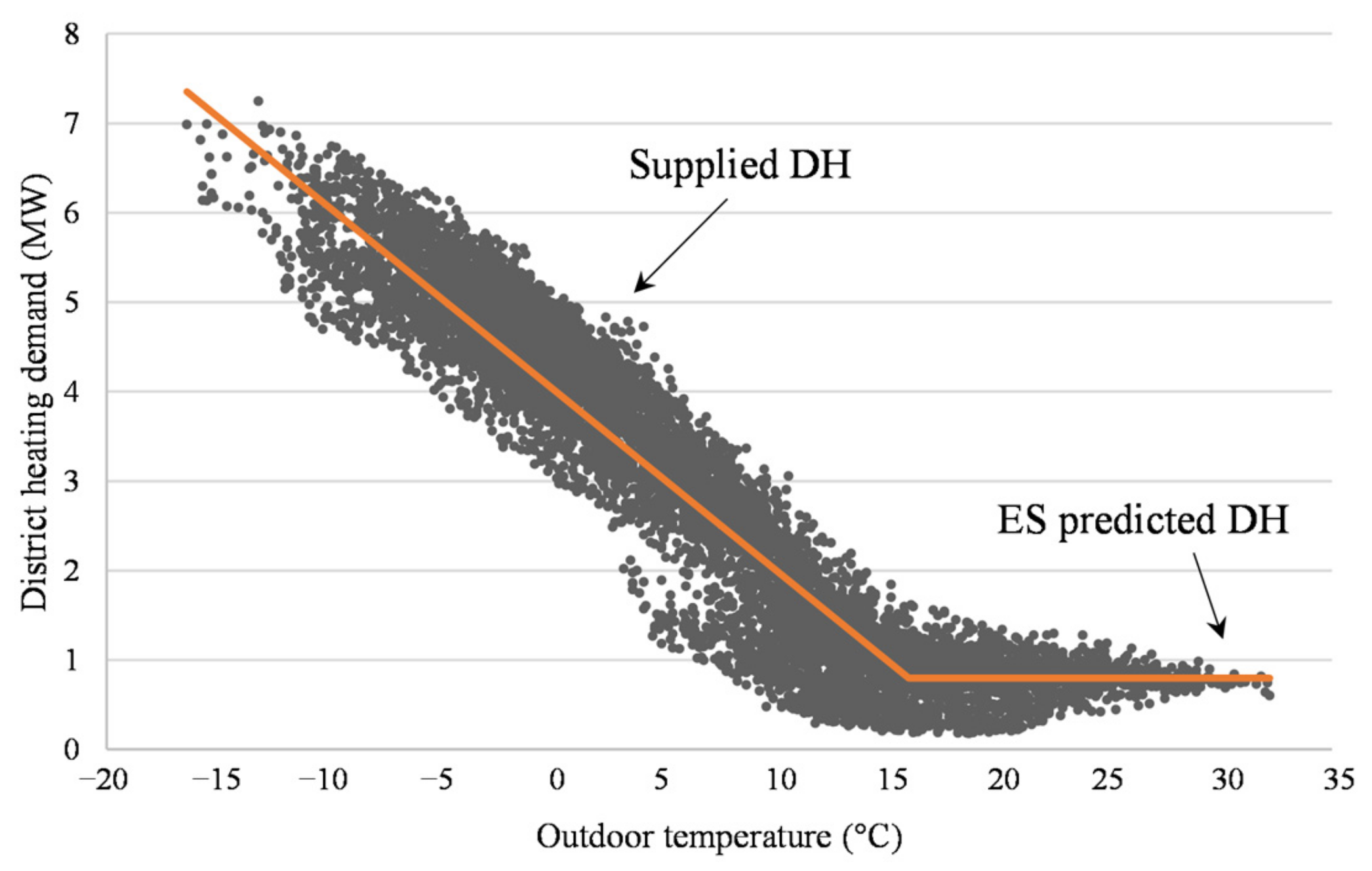
After determining ES parameters, they can be used to calculate energy use on an arbitrary time resolution, where hourly is used in this paper. To calculate predicted DH demand, Equation (2) is used. The plus sign above the parenthesis means that when the difference between T_b and T_outdoor is below zero, the first part of Equation (2) is zero. To determine annual DH demand, P_DH needs to be summed over the whole year. By setting P_dhw and P_dhwc to zero, Equation (2) can instead be used to calculate space heating demand.

$$P_{\mathrm{DH}}=H_{\mathrm{tot}}\ast {\left(T_{\mathrm{b}}-T_{\mathrm{outdoor}}\right)}^{+}+P_{\mathrm{dhw}}+P_{\mathrm{dhwc}}$$

(2)

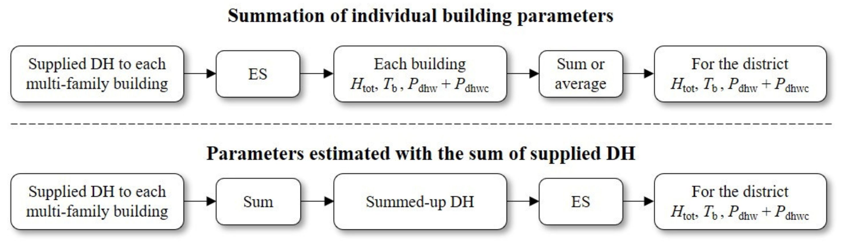
3.2. Predicting Energy Use for the Whole District Using Energy Signature

Predicted energy use for the district building stock was calculated for each building type and the total multi-family building stock. Two ways of determining ES parameters on district level were proposed and compared. The first was to determine ES parameters for each multi-family building individually. Following this, H_tot, P_dhw and P_dhwc are summed, while T_b is calculated as the average of all buildings.

The other way to determine ES parameters was to first sum up DH demand of each building type, and the total for the district multi-family building stock. The summed-up DH demand is then used to determine ES parameters.

Figure 3 shows these methods of determining ES parameters for the multi-family building stock in the district. In the first row of Figure 3, H_tot and P_dhw + P_dhwc are summed, while T_b is calculated as average.

After predicting ES parameters for all multi-family buildings, Equation (2) was used to calculate predicted DH. Annual predicted DH demand was then compared to annual supplied (measured) DH demand.

3.3. Primary Energy Use Number and Simulated Renovation Methodolgy

3.3.1. Description of Primary Energy Use Number

To determine current thermal performance status and to simulate energy renovation, this paper utilises the primary energy use number, called EP_pet. The limit for primary energy use is set by Swedish building regulations according to Boverket (Swedish National Board of Housing, Building and Planning) [52]. The limit applies to several kinds of buildings, although only multi-family buildings are of interest here. Swedish building regulations state that when a building will be renovated, the owner should strive to reduce the building’s primary energy use number to less than the limit set in the recent regulations, which are equivalent to NZEB standard.

In the time of writing this article, the EP_pet limit for multi-family buildings was 75 kWh/(m²∙year) [52]. Calculation of EP_pet for a building is according to Equation (3), which shows the case of space and DHW heating supplied by DH system, and without space cooling.

$$E{P}_{\mathrm{pet}}=\frac{\frac{E_{\mathrm{SH}}}{F_{\mathrm{geo}}}\ast W{F}_{\mathrm{DH}}+E_{\mathrm{dhw}}\ast W{F}_{\mathrm{DH}}+E_{\mathrm{f}}\ast W{F}_{\mathrm{el}}}{A_{\mathrm{temp}}}$$

(3)

where E_SH is space heating energy use, F_geo is geographic adjustment factor, WF_DH is primary energy weight factor for DH, E_dhw is domestic hot water energy use, E_f is facility electricity use, WF_el is primary energy weight factor for electricity and A_temp is heated floor area. The constants F_geo, WF_DH and WF_el are according to building regulations [52]. Geographic adjustment factor for Gävle is 1.1. WF_DH and WF_el have nationally assigned values 0.7 and 1.8, respectively. Additionally, EP_pet should be calculated using normalized data [52]. Normalized data means that energy use must be calculated using typical weather data, normalized occupancy and appliance use, and that annual energy use should be divided by heated floor area, to ensure that the same requirement can be applied on different buildings.

3.3.2. Determining Primary Energy Use Number for Each Multi-Family Building

Primary energy use number, EP_pet, was calculated for each multi-family building, using Equation (3). Following this, it was investigated if EP_pet was within 10% of the limit of 75 kWh/(m²∙year). If true, it was deemed unlikely that the property owner would conduct further energy renovation measures. For these buildings, simulated renovation was not considered. Inputs to Equation (3) are given below.

Space heating demand was calculated hourly using Equation (2). In this case, with H_tot and T_b according to supplied DH, which for the district of Sätra was measured in 2018, and with outdoor temperature according to typical weather data for the city of Gävle. These hourly values were summed to yield annual space heating energy use, and then divided by heated floor area. Facility electricity use, E_f, was gathered from energy performance certificates for each multi-family building. When E_f was missing, average of collected values were used. E_dhw is calculated using the assumption that it is equivalent to base load determined by ES. Converting base load to E_dhw was done by multiplying base load by the number of annual hours. This assumes that base load is constant year-round. This value is then divided by collected heated floor areas, to convert it to kWh/(m²∙year).

3.3.3. Simulating Renovation Using Primary Energy Use Number with the Energy Signature Method

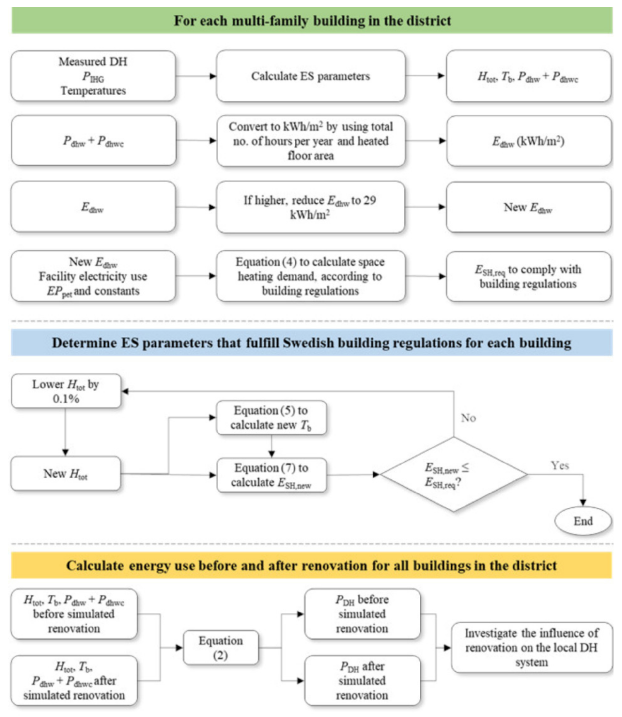
Figure 4 shows an overview of the simulated renovation method used in this paper. The methodology is based on calculating ES parameters, using input values explained in Section 3.1. These parameters along with the primary energy use number (EP_pet) are then used to simulate renovation on the buildings’ base load demand as well as their space heating demand. This is explained below Figure 4.

As mentioned, building base load is made up of DHW and DHWC losses. For DHW losses, the Swedish building energy performance regulation was used as a reference value [53], corresponding to 25 kWh/(m²∙year). Additionally, DHWC losses were assumed to be 4 kWh/(m²∙year), according to Swedish standard value for newly constructed multi-family buildings [54]. The total reference base load is then 29 kWh/(m²∙year). If the base load of a building was higher than this, its base load was reduced to 29 kWh/(m²∙year).

To simulate renovation related to space heating demand, Equation (3) was rearranged to Equation (4), where the constants are specified in Section 3.3.1. E_dhw was set to 29 kWh/(m²∙year), according to the reasoning above. Facility electricity use, E_f, was set as in Section 3.3.2 (gathered from energy performance certificates). EP_pet was prescribed to 75 kWh/(m²∙year). This was done to calculate space heating demand that complies with Swedish building regulations, according to [52]. The parameter is called E_SH,req, to reflect that it is related to Swedish building regulation requirements.

$$E_{\mathrm{SH},\mathrm{req}}=\frac{E{P}_{\mathrm{pet}}\ast A_{\mathrm{temp}}-E_{\mathrm{dhw}}\ast W{F}_{\mathrm{DH}}-E_{\mathrm{f}}\ast W{F}_{\mathrm{el}}}{W{F}_{\mathrm{DH}}}\ast F_{\mathrm{geo}}$$

(4)

The next step of the process was to simulate values for H_tot and T_b after renovation, which is shown in the middle of Figure 4 (with header marked in blue background). H_tot was reduced in steps of 0.1%. For each time H_tot was reduced, a new value for T_b was calculated according to Equation (5).

$$T_{\mathrm{b},\mathrm{new}}=T_{\mathrm{indoor}}-\frac{\mathrm{IHG}}{H_{\mathrm{tot}}}$$

(5)

where T_indoor was set to 22 °C and internal heat gains (IHG) was a constant value calculated for each multi-family building. IHG was calculated using Equation (6). In this case, H_tot and T_b are the parameters determined with buildings’ current energy use, prior to renovation. It is necessary to calculate IHG in this way, in order to retain a starting value that can be used in Equation (5).

$$\mathrm{IHG}=H_{\mathrm{tot}}\ast \left(T_{\mathrm{indoor}}-T_{\mathrm{b}}\right)$$

(6)

For each step that H_tot and T_b were reduced, new total annual space heating energy use, E_SH,new, was calculated according to Equation (7). In Equation (7), typical weather data was used for T_outdoor. E_SH,new needs to be divided by heated floor area in order to convert it to the same unit as E_SH,req, kWh/(m²∙year). Here, also, space heating demand is calculated hourly, and them summed up over the whole year.

$$E_{\mathrm{SH},\mathrm{new}}={\displaystyle \sum }_{i=1}^{8760}\frac{H_{\mathrm{tot},\mathrm{new}}\ast {\left(T_{\mathrm{b},\mathrm{new}}-T_{\mathrm{outdoor},\mathrm{i}}\right)}^{+}}{A_{\mathrm{temp}}}$$

(7)

E_SH,new was then checked to see if it was lower or higher than E_SH,req. If higher, H_tot and T_b were further reduced with the same inputs as described above. With a new reduced H_tot, E_SH,new was calculated and checked, iteratively. The process of reducing H_tot and T_b, using them to calculate E_SH,new, and comparing E_SH,new to E_SH,req was repeated until E_SH,new was lower than E_SH,req.

3.4. Sensitivity Analyses

Several factors were subjected to sensitivity analysis before and after simulated renovation, as explained below.

3.4.1. Before Simulated Renovation

Before renovation, sensitivity analysis was performed on two factors: indoor temperature and internal heat gains, which were used to determine ES parameters. Indoor temperatures were collected for two multi-family buildings of each building type, and were used as inputs to the stock of 95 multi-family buildings. From a large national investigation [55], the indoor temperature variation in multi-family buildings was found to be on average ±0.32 °C. However, in this paper, influence of a deviation of ±1 °C was investigated. Meanwhile, internal heat gains are mostly occupancy dependent, which can vary greatly [56,57,58]. The impact of increasing internal heat gains by 25% was investigated.

3.4.2. After Simulated Renovation

After renovation, three factors were subjected to sensitivity analysis: DHWC losses, indoor temperature and WF_DH. DHWC losses influenced the simulated renovation as shown in Equation (4). It was necessary to investigate changes in these losses, since measurements have shown that these can vary [59]. In addition to the standard value for DHWC losses of 4 kWh/(m²∙year), losses of 2, 8 and 12 kWh/(m²∙year) were investigated. In the same way as before renovation, indoor temperature was varied by ±1 °C, related to Equation (5).

According to Equations (2) and (3), the simulated renovation scheme was also dependent on primary energy weight factors for district heating and electricity. Only differences in primary energy weight factors for district heating, WF_DH, were investigated. WF_DH was given as 0.7 in building regulations [52]. However, for an actual DH system, the primary energy factor depends on local conditions and fuels. Therefore, DH systems in three Swedish cities were investigated: Gävle, Sandviken and Söderhamn, which in 2020 had WF_DH of 0.01, 0.15 and 0.57, respectively [60]. The studied district is in the city of Gävle, and the other two cities were investigated since they are close to Gävle and have similar climates, meaning that the same input data could be used. With these three values for WF_DH, the process described in Section 3.3.2 and Section 3.3.3 where repeated.

4. Results

4.1. Energy Signature Parameters for the District Multi-Family Building Stock

Table 1. ES parameters and difference in annual DH demand, determined for building types and all multi-family buildings in the Sätra district. The difference in DH demand is the difference in demand as predicted by ES against supplied demand.

		Pdhw + Pdhwc (kW)	Htot (kW/°C)	Tb (°C)	Diff. in Annual DH Demand
Tower buildings	Summation of individual parameters	529	131	15.4	3.9%
	Parameters estimated with summed-up supplied DH	535	131	16.1	−0.2%
Low-rise buildings	Summation of individual parameters	261	72	16.0	0.1%
	Parameters estimated with summed-up supplied DH	262	72	16.0	0.2%
All multi-family buildings	Summation of individual parameters	790	203	15.5	2.6%
	Parameters estimated with summed-up supplied DH	797	202	16.0	0.3%

shows the difference of using the sum of individual building ES parameters against determining parameters with the summed-up DH demand. The most significant difference is in prediction of T_b for tower buildings and all multi-family buildings. The difference is likely due to a relatively large difference in T_b between individual buildings, and due to T_b being calculated as average.

In the column to the far right, annual DH demand as predicted by ES is compared to supplied (measured) DH demand. The differences in predicted against supplied DH are low, and using summed-up DH demand yields lower discrepancy. This is in agreement with findings by Powell et al. [61], who found that aggregating energy use dampened individual buildings’ irregular patterns.

4.2. Primary Energy Use Number of the District Multi-Family Building Stock

Using Equation (3) and the methodology described in Section 3.3.2, the number of measuring points within 10% of EP_pet limit of 75 kWh/(m²∙year) was calculated. This was found to be 15 of the 56 measuring points in the district. The majority of these are owned by the municipal building property owner, marked yellow in Figure 2.

For each multi-family building, Figure 5 shows primary energy use number, EP_pet. The colouring is the same as in Figure 2, which has also been inserted as a small-sized version. The horizontal dashed line shows the limit of EP_pet of 75 kWh/(m²∙year) plus 10%. Buildings with primary energy use below this line fall within this limit, and were not considered for energy renovation. Dashed lined bars represent low-rise building while the solid bars are tower buildings. In Figure 5, the different property owners and building types are relatively clustered together. For instance, none of the buildings of the property owner on the far right (in dark blue), fall below the limit. The fifth property owner from the left, in dark red, represent two measuring points of six tower buildings, all of which seem to have undergone renovation.

4.3. Sensitivity Analysis before Simulated Renovation

Before renovation,

Table 2. Impact of changing hourly measured indoor temperature on ES parameters. Displayed for both building types and the total district multi-family building stock.

Tower buildings
	Pdhw + Pdhwc (kW)	Htot (kW/°C)	Tb (°C)
Measured indoor temperature −1 °C	539	136	15.5
Measured indoor temperature	535	131	16.1
Measured indoor temperature +1 °C	532	125	16.6
Low-rise buildings
	Pdhw + Pdhwc (kW)	Htot (kW/°C)	Tb (°C)
Measured indoor temperature −1 °C	263	75	15.5
Measured indoor temperature	262	72	16
Measured indoor temperature +1 °C	260	69	16.6
All multi-family buildings
	Pdhw + Pdhwc (kW)	Htot (kW/°C)	Tb (°C)
Measured indoor temperature −1 °C	802	211	15.5
Measured indoor temperature	797	202	16
Measured indoor temperature +1 °C	792	194	16.6

shows how much the ES parameters are affected by a difference in hourly measured indoor temperature of ±1 °C. H_tot is affected by this change according to Equation (1), which also explains why an increase in indoor temperature leads to lower H_tot. The variation in H_tot is roughly 4%, while T_b increases or decreases by roughly 0.5 °C. Base load, P_dhw + P_dhwc, is determined in relation to T_b, which is why they vary, in this case by less than 1% in all cases. Base load is mostly occupancy dependent, and the small changes in Table 2 are expected.

Table 3. Impact of increasing internal heat gains by 25% on ES parameters. Displayed for both building types and the total district multi-family building stock.

Tower buildings
Internal heat gains	Pdhw + Pdhwc (kW)	Htot (kW/°C)	Tb (°C)
3.1 W/m2	535	131	16.1
3.9 W/m2	539	135	15.6
Low-rise buildings
Internal heat gains	Pdhw + Pdhwc (kW)	Htot (kW/°C)	Tb (°C)
3.1 W/m2	262	72	16
3.9 W/m2	263	74	15.6
All multi-family buildings
Internal heat gains	Pdhw + Pdhwc (kW)	Htot (kW/°C)	Tb (°C)
3.1 W/m2	797	202	16
3.9 W/m2	802	209	15.6

shows how ES parameters are affected by an increase in internal heat gains of 25%, from average values of 3.1 W/m² increased to 3.9 W/m². These internal heat gains are related to Equation (1), where these are called P_IHG. Higher internal heat gains lead to higher H_tot, since the buildings’ corrected space heating demand are then higher. Same as Table 2, base load is the least affected parameter, less than 1%. H_tot increases by roughly 3.5% and T_b decreases by 0.4 °C.

4.4. District Heating Demand before and after Simulated Renovation for the District Multi-Family Building Stock

Figure 6 shows DH demand according to supplied (measured) values to the total district multi-family building stock, in dark grey circles, while the orange line shows DH demand predicted by the ES method. Both are fitted to outdoor temperature in 2018. Predicted DH demand was in this case determined with ES parameters based on summed supplied DH (bottom row of Table 1). Figure 6 shows that the ES method determines a value for H_tot that is roughly average of the supplied DH demand, below T_b. The same applies to base load of the district building stock, above T_b. The total annual supplied district DH demand was roughly 24.7 GWh, and the predicted value by ES was essentially the same, as displayed in Table 1.

Figure 7 shows hourly DH demand predicted by ES, where typical weather data has been used. Solid line applies before renovation and the dashed line after simulated renovation. Figure 7 also show the ES parameters before and after simulated renovation, for all multi-family buildings. With simulated renovation, H_tot decreases by 19%, base load by 15% and T_b by 1.9 °C. Annual DH demand is reduced to roughly 18.6 GWh, a decrease of roughly 28%. Peak power demand is reduced by roughly 1.9 MW.

Figure 8 shows the same data as Figure 7, as a duration diagram, with solid line before renovation and dashed line after simulated renovation. Peak, Middle and Base load periods are fitted to DH demand before renovation. During the Peak, Middle and Base load periods, the average power demand reductions, ΔP_avg, are 1.8 MW, 1.1 MW and 0.4 MW, respectively. The corresponding reductions in DH energy use in each load period are 0.2 GWh, 5.5 GWh and 1.6 GWh.

4.5. Sensitivity Analysis after Simulated Renovation

After simulated renovation,

Table 4. Impact of indoor temperature on ES parameters after simulated renovation. For the total district multi-family building stock.

	Htot (kW/°C)	Tb (°C)
Tindoor = 21 °C	158	14.2
Tindoor = 22 °C	160	14.1
Tindoor = 23 °C	162	13.9

shows how H_tot and T_b are impacted by a difference in T_indoor of ±1 °C, used in Equation (5). Base load is not presented since it is not affected. Overall, Table 4 shows relatively small variations, where H_tot is altered by roughly 1.3% and T_b by 0.2 °C.

Table 5. Impact of domestic hot water circulation losses on ES parameters after simulated renovation. For the total district multi-family building stock.

Domestic Hot Water Circulation Losses	Pdhw + Pdhwc (kW)	Htot (kW/°C)	Tb (°C)
2 kWh/(m2∙year)	655	162	14.2
4 kWh/(m2∙year)	677	160	14.1
8 kWh/(m2∙year)	715	158	13.9
12 kWh/(m2∙year)	740	156	13.8

shows the influence of different values for DHWC losses. Different DHWC losses affect the solution in Equation (4), since it increases E_dhw. The increase in E_dhw will lead to a decrease in E_SH,req, which means that the parameters related to space heating, H_tot and T_b, will decrease. Losses of 4 kWh/(m²∙year) are the reference (standard) value. The largest difference is observed for DHWC losses of 12 kWh/(m²∙year), where base load (P_dhw + P_dhwc) is increased by 9.3%, and H_tot and T_b are reduced by 2.8% and 0.3 °C, respectively.

As mentioned, different primary energy weight factors, WF_DH, were investigated: 0.01, 0.15 and 0.57. This factor is used in Equation (3) to determine the current primary energy use number for each building, thus influencing how many need to be renovated. For the buildings that need to be renovated, WF_DH is then used in Equation (4), to determine a target for space heating demand.

The two lowest values, 0.01 and 0.15, yield results for EP_pet that are far below the mandated limit of 75 kWh/(m²∙year). None of the multi-family buildings in the district require renovation with these primary energy weight factors. Decreasing WF_DH from 0.7–0.57 reduces the number of measuring points that need to be renovated, from 41 to 28. Decreasing WF_DH also increases E_SH,req, as calculated by Equation (4). In turn, the difference between E_SH,new and E_SH,req will be smaller, meaning that the reduction in H_tot and T_b will be smaller. Less renovation related to the multi-family buildings’ space heating demand will be required, and the total DH demand of the district will be higher. Results of the differences between these primary energy weight factors are shown in

Table 6. Different WF_DH and its effects on ES parameters and annual energy use determined with typical weather data, after simulated renovation. For the total district multi-family building stock.

Primary Energy Weight Factor (WFDH)	Pdhw + Pdhwc (kW)	Htot (kW/°C)	Tb (°C)	Annual Energy Use (GWh)
0.57	709	171	14.5	20.2
0.7	677	169	14.1	18.6

. It is clearly seen that lower weight factor increases both ES parameters and the annual energy use of the DH system.

5. Discussion

The simulated renovation methodology proposed in this paper is based on a target for annual energy use, in this case according to Swedish building regulations. In the reduction of ES parameters, base load is decreased to standard value, while H_tot and T_b are decreased with the assumption that these two are correlated according to Equation (5). The relation between H_tot and T_b might be different in real-life situations, with differing occupancy behaviour and internal heat gains. Even so, Park et al. [62] formulated the same equation for calculating T_b as Equation (5) in this paper, and their results showed that reducing H_tot leads to a reduction in T_b.

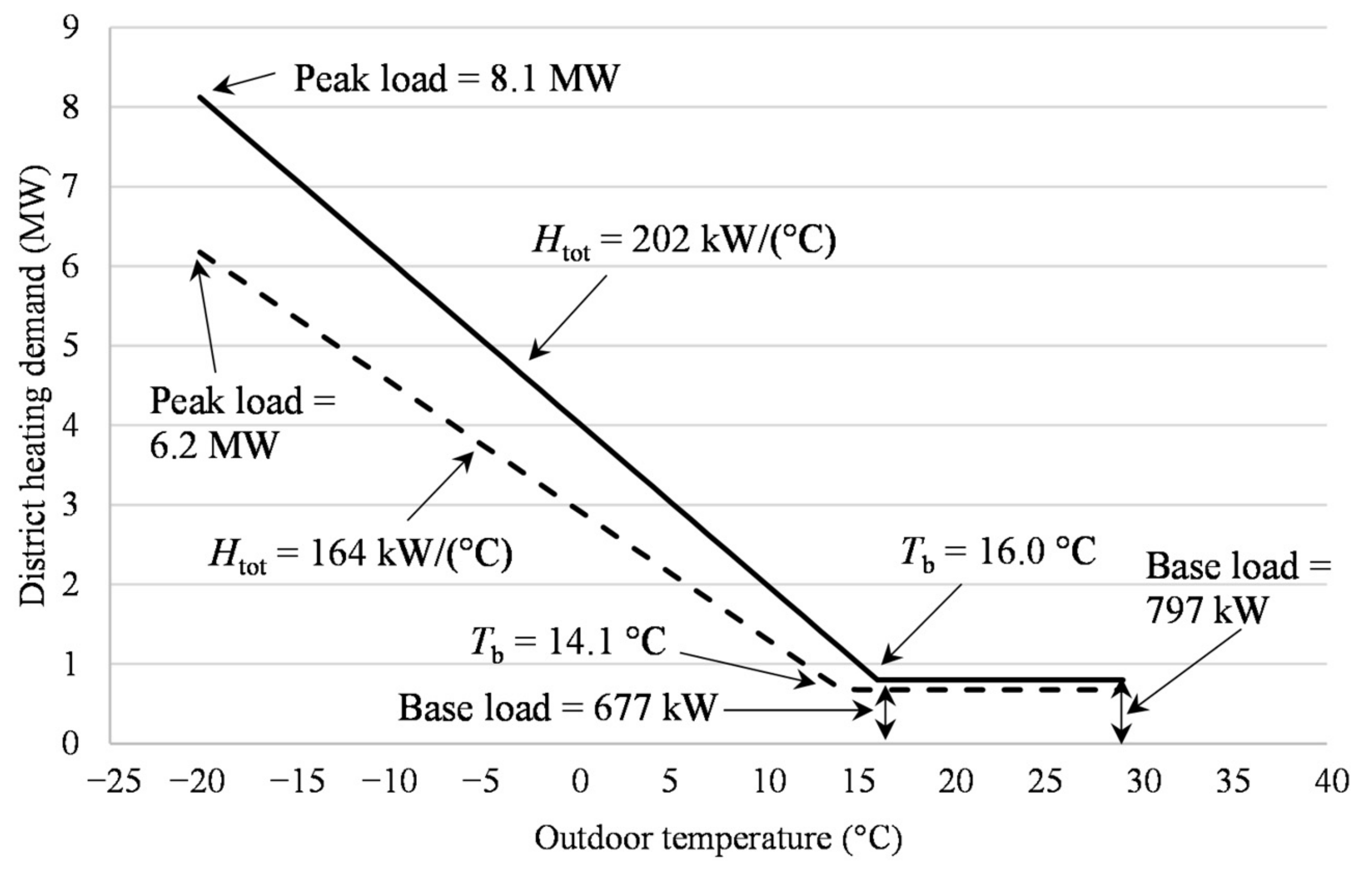
The main findings of this study are displayed in Figure 5 and Figure 8. Figure 5 gives an indication on the thermal performance status of a building, related to Swedish building regulations. This information is vital for building owners, in order to investigate energy use related to these regulations, and if buildings need energy renovation. It can be argued that primary energy use number can be calculated directly using supplied DH, without ES. However, space heating and DHW energy use needs to be provided separately. These were not measured separately in the studied district, which also is the normal in Swedish multi-family buildings. Thus, ES is useful to separate energy use for space heating and for DHW. Individual ES parameters can also be used to prioritise renovation, as to whether energy efficiency measures should be taken on transmission and ventilation losses (H_tot), or losses related to base load (DHW and DHWC). High H_tot suggests that measures should be taken on building envelope and/or ventilation system. High base load could be an indicator for several faults or abnormalities, including leaks or lack of insulation in DHW or DHWC systems piping, or irregular use of DHW by occupants.

Figure 8 is mainly useful for energy providers, since it shows how the renovation of a district can affect energy use in different load periods. In the Peak load period, the reduction in DH power demand (MW) is greatest, compared to Middle and Base load periods. However, the reduction in energy use (GWh) in Peak load period is relatively small, due to its short length of only 100 h. This is compared to 5100 h for Middle load period and 8760 h for Base load period. Despite this short length, it is relevant for DH companies to reduce Peak load. Peak load is usually covered by renewable or fossil oils, which have high running costs and carbon dioxide (CO₂) emissions [63,64,65]. Meanwhile, reduction in the Middle load period leads to reduced operation of the biofuel CHP plants, which may have negative effects on economic factors and CO₂ emissions [64]. This is because the production of electricity in CHP plants is linked to heat demand in the DH system. Thus, in Gävle, decreased DH demand in buildings can lead to decreased electricity production. This can lead to increased or decreased CO₂ emissions, depending on what assumptions are made regarding marginal electricity and if envelope energy efficiency measures are combined with electricity saving measures [65].

One of the major advantages of this method is the CPU time, which takes only ten seconds to determine ES parameters for each building, while simulating renovation for the district multi-family building stock only takes three seconds, using university remote server. However, at the moment the method for simulating renovation has not been validated against any real buildings. We have also not investigated what measures are required to decrease H_tot by, e.g., 20%, which is a potential topic for further research.

The sensitivity analyses performed, both before and after simulated renovation, show that the newly developed ES method is insensitive to changes in indoor temperature. Here, the excess indoor temperature difference of ±1 °C was used. It is necessary to investigate different indoor temperatures, since these can vary in and between buildings, and because measured indoor temperature is lacking for the majority of Swedish multi-family buildings. The simulated renovation was also checked for different values for domestic hot water circulation losses (DHWC). With an increase in DHWC losses of 200%, Table 5 shows that only base load is significantly affected, which is expected since DHWC losses are part of the base load. DHWC losses have been shown to vary significantly [59], and it seems that more research is needed on how to predict these losses and how to assist property owners to reduce it. The developed ES method is capable of estimating DHWC demand (P_dhwc), assuming that energy use is measured on hourly basis and not rounded to nearest tens.

How primary energy weight factor for district heating (WF_DH) affects district renovation is also investigated. WF_DH is mandated on national level, and has a value of 0.7, which is compared to local values in three cities. Two cities had WF_DH of 0.01 and 0.15, since they primarily use industrial excess heat and secondary biofuels. With these low values, none of the buildings in the district need to be renovated, using the method derived from Swedish building regulations. For the third city with WF_DH 0.57, the number of buildings that need to be renovated decreases, and the level of renovation decreases for these buildings. If these local values are used instead of the nationally mandated ones, the current way of calculating primary energy weight factor, which is meant to promote energy efficiency in buildings, should be altered. This suggests that the issue of energy renovation in buildings is more complicated than to simply reduce the buildings’ energy use as much as possible and that local conditions should be considered. Even if low WF_DH suggests that renovation is not needed, energy renovation should be performed. For one, biomass and other resources used in DH systems can be freed up for other uses. Many Swedish cities with DH systems are also growing, which means that renovation of the old building stock saves energy that can be used in new buildings.

Electricity demand is also included in the calculation of primary energy use number, Equation (3). With lower WF_DH, the share of electricity demand will increase. For the studied multi-family building stock, WF_DH of 0.01 increases the average share of primary energy for electricity to more than 90%, and with WF_DH of 0.15 the share is equivalent to more than 50%. A further aspect of electricity demand is that to reduce the space heating demand of a building, it might be necessary to install a ventilation system with heat recovery. This increases total electricity demand and affects primary energy use [66,67]. For the district multi-family building stock, changing ventilation system has not been considered. Figure 7 shows that the decrease in H_tot is only about 20%, which likely can be achieved without measures in the ventilation system.

In a similar way as we have done in this paper, Pasichnyi et al. [23] used ES to model energy use of buildings, and for the majority of their studied buildings, they found good agreement between measured and modelled values. Sjögren et al. [68] studied energy use of 96 multi-family buildings with an ES method, in another Swedish city. Unlike the findings in this paper, they found that increasing indoor temperature leads to an increase in H_tot. The parameters they investigated were for individual buildings, while this paper mostly looked at district level.

Some limitations that should be mentioned are that data was not always available for individual multi-family buildings, data was sometimes rounded to nearest tens (kW) and that the simulated renovation measures have not been related to actual measures in multi-family buildings. Since some of the multi-family buildings shared the same DH substation, data was not always available for individual buildings. This could limit the results since if, for example, four buildings share the same substation, it is possible that only three of these buildings have undergone renovation, sufficiently lowering the energy use in the substation so that all four appear to be renovated. Even so, if it is necessary, earlier renovation actions can be confirmed by visual inspection or by contacting the building owner. Rounded data is mainly a limiting factor when estimating parameter for individual multi-family buildings, and less so when using data on a district scale. Reduction in heat loss coefficient is simulated based on building regulations. However, it has not been estimated which physical measures are required to achieve the decrease. This limitation has also been highlighted as a potential for future research for data-driven methods in general [44]. Information on physical renovation measures is potentially even more useful to building owners, than to only know that their buildings need to undergo renovation.

We have also not investigated potential influence of well-known rebound effects, concerning additional impacts of behavioural effects on the practical outcomes of energy renovation measures [69,70]. Increasing indoor temperature is a rebound effect that has been widely reported, which reduces the benefit of energy renovation [71,72,73]. Other factors that can cause rebound effects include incorrect adjustments of the heating system, oversized heating system and over-ventilation [71]. While rebound effects can be related to increasing consumption levels, the most relevant effects in this paper are those directly or indirectly related to electricity, space heating and hot water use. For the studied district of Sätra, rebound effects due to occupancy behaviour are expected to be low. This is because the occupants have limited influence on the indoor climate in the buildings, since it is centrally controlled by the heating system, a common practice in Sweden [74,75]. To finance renovation, it is also common for building owners to increase rents, which means that occupant consumption related to energy use is not expected to increase.

Conversely to the rebound effect, Sunikka-Blank and Galvin [76] introduced the prebound effect, which refers to a situation where the energy use of a building, before renovation, is lower than calculated energy use. This can reduce expected energy use savings, and impact financial feasibility [77,78,79]. The uncertainty of prebound effect should not affect the results of this paper in a significant way. This is because the ES method is based on measured data, in this case district heating, where effects of occupancy presence and other uncertainties, present in physical (law-driven) methods, are already included.

6. Conclusions

This paper demonstrates how the information from the energy signature (ES) method can be useful to building owners and energy providers. The ES method is used to determine the current primary energy use of each multi-family building in a district, which shows if a building needs to be renovated in order to comply with Swedish building regulations. Additionally, ES is used to simulate renovation for the district stock of 95 multi-family buildings, related to the same building regulations. The effects of renovation are studied using a duration diagram, revealing how different load periods are affected in the local district heating (DH) system.

The current primary energy use, along with ES parameters, contains information that is useful to building owners, since it can guide renovation measures that should be taken. Meanwhile, since the load periods in the duration diagram are related to the operation of local DH system plants, the method is demonstrated as being useful to energy providers.

While other studies in Sweden have used time-consuming engineering methods or only investigated individual buildings, this paper uses a statistical method to provide information on dynamic energy use before and after simulated renovations. Sensitivity analysis is also performed, showing that the method is insensitive both before and after simulated renovation, to variations in factors such as indoor temperature and internal heat gains. The simulated renovation is also dependent on primary energy weight factor for DH, which is subjected to sensitivity analysis. The nationally mandated DH primary energy weight factor is used, as well as local values from three cities with similar climates. It is found that lower primary energy weight factor decreases the simulated renovation level, or even negates any need for renovation.

The method could also be used for other building stocks, where space heating demand dominates building energy use, such as in the Nordic countries. To simulate renovation, the paper used the limit for primary energy use as set by the Swedish government agency responsible for community planning, construction and accommodation, Boverket. With this method, renovation of the district multi-family building stock is performed according to nearly zero-energy building standard, outlined in the Energy Performance of Buildings Directive as a way to achieve a decarbonised building stock [2].

For the research method and results of this study, the authors have identified the need and potential for the following future research:

• Economic consideration. It has not been investigated if renovations are profitable. This could be based on life cycle cost assessment, accounting for the life span of technical installations and building materials.
• Investigate how the total heat loss coefficient, called H_tot, can be divided into its constituent parts, regarding transmission, ventilation and infiltration losses. For an ES methodology developed in [43], it is suggested that this could be achieved by correlating wind speed data and heat losses.
• The method should be used and assessed on a larger scale, with a larger amount and different types of multi-family buildings and districts. Future investigation can employ data for the Swedish city of Gävle, used in this paper, or other cities.
• In addition to investigating a larger building stock, Deb and Schlueter [44], suggested that there is a lack of studies on data-driven methods where measured building data is available both before and after renovation, for example performed in [80].
• Estimating greenhouse gas emissions. Since the building sector is responsible for a large share of emissions, it is necessary to investigate the reduction related to energy renovation measures and the local energy system.