Abstract
This work aims at investigating the effects of forest heterogeneity on a wind-turbine wake under a neutrally stratified condition. Three types of forests, homogeneous (idealized), a real forest having natural heterogeneity, and an idealized forest having a strong heterogeneity, are considered in this study. For each type, three forest densities with Leaf Area Index (LAI) values of , and are investigated. The data of the homogeneous forest are estimated from a dense forest site located in Ryningsnäs, Sweden, while the real forest data are obtained using an aerial LiDAR scan over a site located in Pihtipudas, about 140 km north of Jyväskylä, Finland. The idealized forest is made up of small forest patches to represent a strong heterogeneous forest. The turbine definition used to model the wake is the NREL 5 MW reference wind turbine, which is modeled in the numerical simulations by the Actuator Line Model (ALM) approach. The numerical simulations are implemented with OpenFOAM based on the Unsteady Reynolds Averaged Navier–Stokes (U-RANS) approach. The results highlight the effects of forest heterogeneity levels with different densities on the wake formation and recovery of a stand-alone wind-turbine wake. It is observed that the homogeneous forests have higher turbulent kinetic energy (TKE) compared to the real forests for an LAI value less than approximately 2, while forests with an LAI value above 2 show a higher TKE in the real forest than in the homogeneous and the strong heterogeneous (patched) forest. Technically, the deficits in the wake region are more pronounced in the strong heterogeneous forests than in other forest cases.
1. Introduction
The assessment of forest properties in the numerical modeling of Atmospheric Boundary Layer flow (ABL) in wind parks is becoming extensive in Computational Fluid Dynamics (CFD) applications, especially in wind resource management. Although forest density varies in space with vertical and horizontal directions, it is almost always assumed to be horizontally homogeneous with a fixed canopy height in numerical simulations [1,2,3,4]. Real forests have heterogeneous properties with different canopy morphologies, such as tree heights and shapes, and their corresponding bio-mass areas. The local details of individual trees from real forests have inspired an investigation to know if the homogeneous description of forest in CFD numerical simulations is accurate enough to account for wind-turbine wake flow in forested wind farms.
There are two main approaches whereby tree effects can be accounted for in CFD numerical simulations: the implicit method where the impacts of trees are modeled by using the surface roughness length and the displacement height; and the explicit method where the porosity of the forest canopy is modeled to account for the presence of trees in the domain. Mohamed et al. [5] established the fact that while the modeling of trees in the numerical studies of wind flow is important, the explicit method has remarkable details of trees compared to the implicit method. Forest canopy can be modeled explicitly in CFD models by including a source term in the momentum equations. The source term consists of the dimensionless drag coefficient, forest leaf area density (LAD) distribution of individual trees, and the local velocity magnitude [6]. Most CFD simulations with forest inclusion are carried out using the explicit approach for tree representation. In several studies [5,6,7,8,9,10] and many others, tree representations are mostly assumed to be horizontally homogeneous with a constant leaf area density (LAD) throughout the computational domain. This assumption is mostly made because of the difficulty in obtaining accurate information about real forest structure. Nonetheless, a few studies have used real forest data in CFD simulations [2,11,12]. For example, Boudreault et al. [11] implemented the canopy structure by utilizing an aerial LiDAR scanned data as frontal area density with the Beer–Lambert law [13]. The LiDAR method provides the ability to assess the canopy structure and gives more accurate predictions of ABL flow over forests. This method gives rise to great variability of wind field within and above forest canopy. From the findings in [11], the high variabilities observed in the stream-wise direction showed a substantial dependence on the terrain features, but obvious effects of the forest heterogeneity were also observed. Recent research on the numerical modeling of neutral ABL flow through heterogeneous forest canopies also reveals that the homogeneous forest has higher turbulence intensity compared to a heterogeneous forest [14]. In addition, Desmond et al. in their study [2] showed that a detailed evaluation of forest properties, that is the heterogeneity of forest, enhances the accuracy in the modeling of ABL flow over forests.
The study cases in this work are designed in a way that a stand-alone wind turbine is situated amid a fully forested area such that the flow develops over the forest before the turbine. Even though the high level of turbulence created by the forest increases the mechanical loads on wind turbines [1], many are yet situated in or near forests because of relatively low installation costs and due to public acceptance [15]. Furthermore, the increased turbulence intensity levels of the upstream flow (in our case, influenced by the forest drag) lead to a considerable influence on the spatial distribution of the mean velocity deficit, TKE, and turbulent shear stress in the wake region [16]. Usually, when the turbulence levels are higher in the upstream ABL flow, the turbine-wake recovers faster, and the maximum TKE increase is close to the upper tip of the turbine rotor [4,16]. A detailed analysis of these features in different forest configurations will be carried out in this study. This study will enable an investigation that can help in developing a more efficient management of wind resources on wind farms.
Our study examines the heterogeneity effects in the upstream ABL and turbine-wake flow over different forest densities. To achieve the aim of this study, varying densities of homogeneous and heterogeneous forests are simulated. The homogeneous forest is composed of the Scots pine (Pinus sylvestris) trees with uniform densities based on the leaf area index (LAI) of individual trees. The forests are assumed to be horizontally homogeneous but with varying LAD distribution in the vertical direction. On the other hand, a real forest composed of different types of trees, representing a mixed forest with uneven spacing between individual trees, is considered to ensure that the three-dimensional information of the forest is naturally heterogeneous. A third case of a highly heterogeneous forest was further created artificially from the real forest data, where small forest patches were generated by alternating a field of zero LAI and a small patch, which was twice the mean LAI of the real data. This case can be likened to a patched forest and thus is referred to as patched forest in this study. The LAIs of the respective forest cases are , and , which represent extremely sparse forests, medium sparse forests, and dense forests. These three LAI cases were chosen based on the ABL flow simulation analysis carried out previously by the same authors [4], where the cases were shown to have clear distinctions in the turbulence kinetic energy (TKE) generation with respect to LAI.
The numerical modeling of air flow, especially when considering forest canopy heterogeneities that entail rapid changes of LAI across the domain, are best computed using the Large-Eddy Simulations (LES). LES have been proven as an efficient technique since it gives more essential information on instantaneous fluctuations of the flow quantities. On the other hand, the Reynolds-Averaged Navier–Stokes (RANS) technique solves the time-averaged quantities of the flow equations, and the solution produces the mean flow quantities. Hence, the two-equation RANS turbulence models are unable to accurately capture the resulting non-equilibrium states of turbulence. Nonetheless, RANS, when compared with LES, has emerged to be a more affordable approach that gives reliable predictions about the flow characteristics. Precisely, RANS has been used to carry out numerical studies of forests’ effects on the ABL flow [4,10,17,18] and to model wind-turbine wake in the ABL, e.g., [19,20,21,22] among others.
The Unsteady-RANS approach, using the realizable turbulence model, is employed in this study, and all simulations are performed using OpenFOAM [23]. The wind-turbine wake is modeled using the specifications of the NREL 5 MW reference wind turbine with a rotor diameter of 126 m [24], which is simulated using the Actuator Line Model (ALM) [25].
2. Forest Descriptions
The forest density is modeled using LAD distribution of individual trees, and the cumulative LAI is defined as,
where h is the maximum height of the forest and is the vertical LAD profile data.
2.1. Homogeneous Forests
The forest density used as the homogeneous forest in this study is digitally extracted from the report of a field experiment performed by Arnqvist et al. [26]. The forested land largely comprised of Scots Pine (Pinus Sylvestris) trees, with an estimated mean forest height of m. The terrain in the forest site is mainly flat with insignificant variations. Detailed information about the experiment is well documented in the final report [15]. The LAD profile derived from this experiment has been applied in several numerical studies [1,4,27,28]. The extracted data match with a dense pine forest with LAI , and it represents the reference forest from which the remaining two forest densities are estimated. The first case is estimated by reducing the LAI of the reference forest by 10 times to represent a very sparse forest, while the second case is of the reference forest density to represent a medium sparse forest. Figure 1 shows the LAD distribution of individual trees in the respective forest cases considered with their corresponding LAI values.
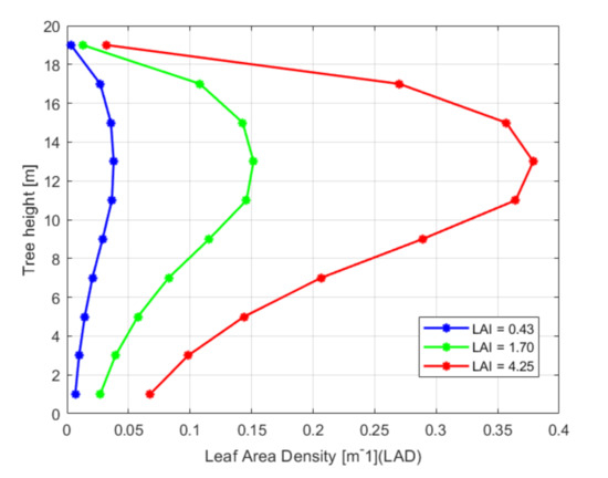
Figure 1.
LAD distribution of individual trees in the respective forest cases considered.
2.2. Real Forests
To characterize the heterogeneity of the forest, we use the raw point cloud data obtained using an aerial LiDAR scan of the land surface over a Finnish forest site composed of mixed forests. The location of the forest site is Pihtipudas, north of Jyväskylä, Finland. The ground was flattened to eliminate the terrain effect in the data. The area contained rasters with 5 m pixel size at every 2 m height. The projected land area and the Google map is presented in Figure 2. The projected land area has grid cells, while the computational domain used in this study is designed to be grid cells. Therefore, it is expedient to slice a part out in the y-direction and repeat a part of the x-direction to have a forest site that suits the numerical domain. This modification may cause some visual dissimilarity between the aerial photos presented in Figure 2 and Figure 3, when compared with the 2D LAI map (see Figure 4). Nonetheless, the nature of the real forest data is preserved with a little repetition toward the right-end in the numerical set-up.
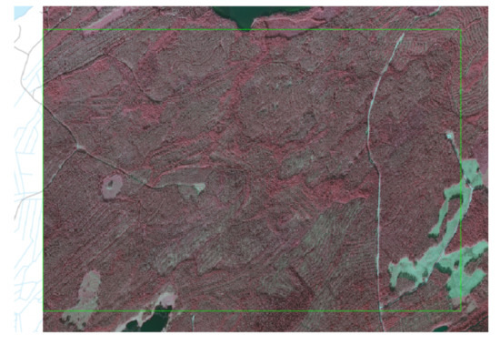
Figure 2.
Projected land area showing the location covered.

Figure 3.
Google map picture with red borders showing the location covered.
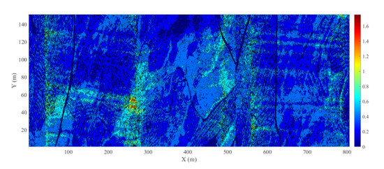
Figure 4.
Two-dimensional (2D) LAI map for real forest with mean LAI .
The LAI of the LiDAR data originally has a mean value of approximately . Then, the data were rescaled with a factor of 4 and 10 to generate two more cases of real forests having their mean LAIs matching with the corresponding case of homogeneous forests (see Table 1). The three-dimensional distribution of the forest properties showed a very high heterogeneity in the data. Trees of thick canopies and sparse trunk space are equally contained in the data. The maximum height of the trees contained in the data is 20 m.

Table 1.
Description of forest cases with respect to the (mean) LAI.
2.3. Patched Forests
The real forest data were further modified to create a patched forest composed of small homogeneous forest patches. This was achieved by dividing the forest area into square patches of size () m and alternating the LAI in these patches between 0 and twice the mean of the respective LAIs. The aim is to have another forest configuration with higher heterogeneity to be able to justify our findings on the effects of forest heterogeneity on ABL and on the wake flow. Three density cases of LAI are generated for this configuration. Figure 5 represents the 2-D LAI map for the patched forest.
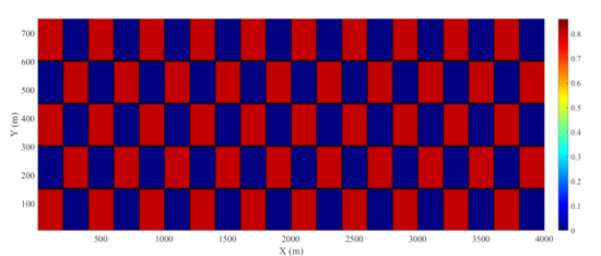
Figure 5.
Two-dimensional (2D) LAI map for patched forest (idealized strong-heterogeneous forest) with mean LAI = 0.43.
For identification purpose, all cases are described in Table 1 with respect to the LAI (density).
To assess the variability in different forest cases, the mean () and standard deviation () of the forest LAI are shown in Table 2. These are statistical parameters that can be used to describe the level of variability in the forest data for respective cases. The patched forests have the highest while the real forests have less . The smaller in the real forest data shows the relatively low variability in the point cloud data. In most cases, the natural vegetation cover of the forests or the presence of broadleaves homogenizes the distribution of LiDar scanned values, which leads to more values grouped around the mean [29].
Table 2.
Mean () and standard deviation () of LAI for respective forests.
The normalized probability distributions for all cases are presented in Figure 6.

Figure 6.
Normalized probability distributions of the LAI for all forests cases.
3. Modeling Approaches
The Unsteady Reynolds Averaged Navier–Stokes (U-RANS) technique is employed in this study, where the Navier–Stokes time-averaged equations of the flow are solved. The unsteady, incompressible form of the equations is given as
is the mean velocity vector in the component notation, is the density, P is the mean pressure, is the viscosity, is the eddy viscosity, and are the two body source terms needed for the forest canopy and turbine wake modeling, respectively. The forest is parameterized in the simulations through the forest canopy model (FCM) using momentum sink term as proposed by Shaw and Schumann [6]. This represents the distribution of forest drag force (due to forest canopy elements) that depends on the vertical shape and density of the forest;
where the drag coefficient , is the LAD profile data, is the magnitude of the mean velocity vector, and is the i-component of the mean velocity.
Since the study is based on the RANS method, turbulence generation and dissipation within the computational domain is parameterized by using the two-equation turbulence model. Specifically, the realizable turbulence model is utilized for the turbulence modeling [30]. The transport equations for TKE, k, and its dissipation, , are given as
where
and
denotes the TKE generation due to mean velocity gradients, while is the TKE generation due to buoyancy. The model constants are . and are source terms added to model the influence of trees on the turbulence. , and are functions of the velocity gradient. The source term added in the k equation is:
The constant models the turbulence production associated with the drag force due to canopy elements, while models the associated dissipation. The source term added in the equation is
where and are model constants.
Although LES captures most of the turbulent fluctuations of the flow parameters unlike RANS, nonetheless, RANS is more affordable in terms of computational cost and time, and the results have also been proven reliable to describe the mean flow quantities of ABL flow over forests [4,10,17,18].
3.1. Actuator Line Model (ALM)
The ALM technique, proposed by Sorensen and Shen [25], was designed to simulate wakes of wind turbine(s) using the blade element theory. The method is such that the body forces are distributed on the actuator line elements to model turbine blades. Each blade is discretized into a series of actuator points called blade elements, and the body forces on these elements consist of the lift () and drag () forces acting on blade cross-sections and are determined using two-dimensional airfoil data. The lift and drag forces acting on the actuator points are defined based on local wind speed () relative to the rotating blade section, angle of attack (), the chord length (c), and the thickness of the blade element (d) in the span-wise direction. However, the effects of these forces on the ABL flow defined in the grid points are modeled by a distributed turbine force vector defined as,
where r is the distance between the location of an actuator point center to the point where the body force is applied, and is the smearing width, which is used to adjust the concentration of the distributed load. Smearing helps to distribute the forces in a way to maintain numerical stability. In this study, the parameter is selected to be twice the local grid spacing, and this has been proven by many authors as the minimum size recommended to obtain a good compromise between accuracy and eschewing oscillations in the wake flow [31,32,33,34]. Forty actuator points are considered along the blade, and the tip-root loss corrections based the Glauert tip loss corrections model [35] is applied in the simulations. The turbine force vector is added to the momentum Equation (3) as sink term ().
3.2. Turbine Information
The reference wind turbine (NREL 5 MW) developed by the National Renewable Energy Laboratory (NREL) is a virtual utility-scale turbine with a power rating of 5 megawatt (MW), which is suitable for onshore and offshore wind energy modeling operations. In this study, the hub height (H) is taken to be 110 m due to the 20 m tall forest included in the computational domain. The turbine has a rotor configuration of three blades, with rotor diameter m. The lift and drag coefficients of the airfoils used in modeling the turbine were provided in the full documentation of the 5 MW reference wind turbine [24]. Although the NREL 5 MW has been utilized for this study, the methodology used in this study can also be applied to any other turbine specification.
4. Simulation Techniques
This section describes in detail the techniques applied in the numerical set-ups in this study. The validations of methods and techniques are further presented in Section 4.1.
Following Mendoza et al. [36], the dimensions of the domain, presented in Figure 7, are taken with respect to the turbine rotor diameter ( m) as in the stream-wise (x), in the span-wise (y), and in the vertical (z) directions. The turbine location is chosen to be downstream of the inflow boundary with a hub height m. The domain has grid spacings of 5 m in the x and y directions and 2 m in the vertical direction within the forest canopy, above which the grid is stretched with a factor of m (2:5) to the top of the domain. This led to cells in the , and z directions, respectively. Furthermore, the computational grids cells are refined in the turbine rotor area, from before the turbine to after the turbine in the stream-wise direction, and from the forest canopy height to above the upper rotor-tip in the z direction. Hence, the grid cell size in the rotor area is approximately m in all three directions.
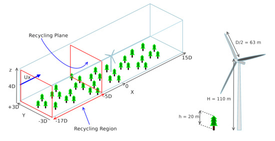
Figure 7.
Computational domain.
Using the recycling method described by Baba-Ahmadi and Tabor [37] to obtain a neutrally stratified ABL profile, the upstream flow is recycled within a length of between the inflow plane and the recycling plane, while a buffer zone of is defined from the recycling plane to the turbine location. The recycling method has been used for ABL development in existing studies [4,8,36,38,39,40].
The wall functions are applied on the terrain while the periodic BC (cyclic) is used along the span-wise direction. The terrain roughness length is set to m. The velocity upstream of the turbine is approximately 10 ms at the hub height. The recycling method is further portrayed on the sketch of the computational domain presented in Figure 7, and the fully developed inflow profiles generated with the method are presented in Section 5.1.
The Unsteady-RANS simulation was implemented by utilizing the pimpleFoam solver [23] in OpenFOAM. The pimpleFoam solver is a RANS-based turbulent flow solver efficient for transient simulations in OpenFOAM. The method is based on the Semi-Implicit Method for Pressure Linked Equations (SIMPLE) and the Pressure-Implicit with Splitting of Operators (PISO) algorithms. The implicit, second-order backward time scheme and the second-order central differencing scheme for spatial discretization implemented in OpenFOAM are applied. Nine forest cases with LAI values of approximately , , and for homogeneous and heterogeneous forests are simulated. Each simulation has a total run time of 6600 s, and a fixed maximum Courant number of is maintained in all cases. The simulations were executed in two phases: the first phase of the simulations was run for the first 5400 s of flow time without turbine and without mesh refinement. This helps to achieve a fully developed ABL flow over respective forests before the turbine is included. In the second phase, the turbine was included (with refined mesh), and the simulations were continued for another 1200 s of flow time, where the last 600 s is meant for taking the field average of the flow quantities. Although it was verified from the instantaneous mean flow quantities that 6000 s of simulation time was statistically adequate to achieve stationary mean quantities in the wake flow, it is discovered that field averaging is necessary to avoid local error due to blade rotation at the turbine location. Meanwhile, the local error does not appear at locations farther downstream of the turbine. Using 384 and 512 parallel processors respectively for the first and second stage of the simulations, it takes approximately and h of clock time for 5400 s and 1200 s of flow time, respectively. Thus, the total simulated flow time (6600 s) takes approximately h of clock time with about variations in different cases. The summary of the methodology is presented in Figure 8.
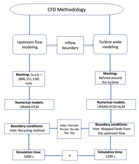
Figure 8.
CFD methodology flowchart.
All computations are carried out on the Mahti server of the Finnish supercomputer managed by CSC-IT for Science.
4.1. Validation of the Numerical Methods and Techniques
The methods and techniques used in this present study have been tested and validated in a previous work carried out by the same authors [4].
The mesh independence test was performed by investigating three different grid resolutions on the NREL 5 MW reference wind turbine. Mesh resolution is crucial in simulations with the RANS technique, since it affects the result accuracy, especially in turbine simulations where the effect of the blade rotation has to be predicted. Therefore, grid spacings of , , and m are tested separately on the refined (wake) region of the computational domain. The quantitative effect of the different grid resolutions on the wake region are presented in Figure 9 and Figure 10. The results are normalized by the velocity at the hub ().

Figure 9.
Vertical profiles of stream-wise velocity from the midplane for different mesh resolutions (the shaded region depicts the rotor area) [4].
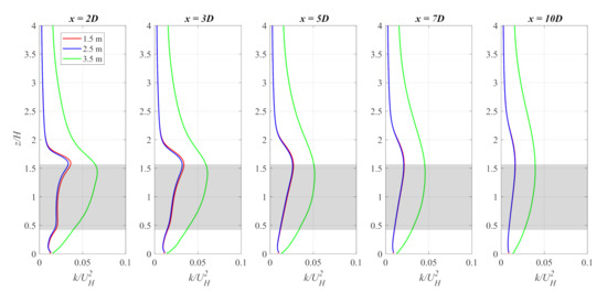
Figure 10.
Vertical profiles of TKE from the midplane for different mesh resolutions (the shaded region depicts the rotor area) [4].
Considering the wake characteristics, the results show that m resolution did not produce considerable improvements from the m resolution, especially at locations. In addition, the power output and aerodynamic thrust from the three different mesh resolutions are compared with the NREL 5 MW benchmark data, which were extracted at exactly 10 ms wind speed [24]. The percentage errors of the power output and aerodynamic thrust for the mesh independence study are presented in Figure 11. Table 3 shows the computational cost in terms of the number of cells, number of processors, and execution time for each mesh resolution. The m resolution under-predicts the power output with , while the m resolution has a better agreement with an over-prediction of , and the m resolution has a better agreement with an under-prediction of . Considering the thrust output, all the three meshes under-predict the thrust when compared to the benchmark data of the NREL 5 MW. The results show about error in the m resolution, deviation in the m resolution, and error in the m resolution.
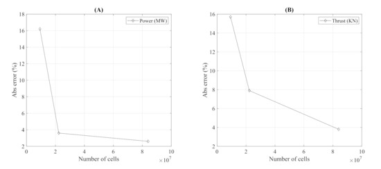
Figure 11.
Percentage error of power (A) and thrust (B) of each mesh resolution from the NREL 5 MW data.
Table 3.
Mesh independence test on NREL 5 MW.
Although the m resolution gave a better agreement with the benchmark data, it is computationally more efficient to use the m mesh resolution since the percentage error is much less than . Therefore, we find it optimal to use the m resolution to obtain a balance between computational efficiency and reliable results. In addition, similar grid resolutions have been proven sufficient to resolve the blade elements of the turbine rotor model (ALM) and the flow after it [1,8,41].
Furthermore, the forest canopy model was validated against the measurements from the Vindforsk III project V-312 [15,26]. The forest case presented in the experimental work is utilized as the reference forest (H10) in this present study; thus, H10 was modeled, and the results were compared with the measurements from the experiment. Figure 12 shows the vertical velocity and TKE profiles from the modeled case and the measurements. The results show that the modeled data underestimate the TKE with about discrepancy, and the mean velocity was also underestimated above with approximately deviation from the measurements. With observations that the modeled results are within the confidence interval estimate of the measured data, it can be inferred that there is a good agreement between the modeled data and the measurements.
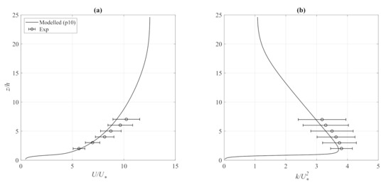
Figure 12.
Vertical velocity (a) and TKE (b) profiles of the modeled case (H10) and the measurements taken from the midplane.
Lastly, the wake simulations were validated against wind-tunnel measurements of a small-scale wind-turbine wake. As there are no data for the virtual NREL 5 MW wind turbine available for validation purposes, a wind-tunnel experiment performed by Chamorro et al. [42] was mimicked using the U-RANS approach. The small-scale modeling helps to validate the modeling techniques applied in the study. The inflow profile of the mean velocity (Figure 13a) shows a maximum discrepancy of observed at between the simulation result and the experimental data. Meanwhile, the turbulence intensity (I) profile presented in Figure 13b is under-predicted below with a maximum discrepancy of about observed at . From Figure 14, the stream-wise velocity profiles in the near-wake region () indicate some level of mismatch with maximum disparity of observed at the hub height. Nonetheless, the turbulence intensity profiles in the wake region show a better agreement between the experimental measurements and the simulations. The maximum difference of about at is observed at the location. Overall, from the wake results presented in Figure 14 and Figure 15, the deviations reduced, and the errors became negligible as the wake-flow recovers downstream. The details of the small-scale wind-turbine simulations can be found in [4].
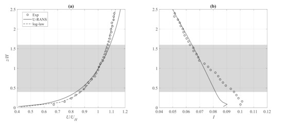
Figure 13.
Vertical profiles of the upstream mean velocity (a) and TKE (b) from the midplane (the shaded region depicts the rotor area) [4].

Figure 14.
Vertical profiles of mean velocity normalized with the hub-height velocity at different stream-wise locations downstream of the turbine taken from the midplane (the shaded region depicts the rotor area) [4].

Figure 15.
Vertical profiles of turbulence intensity (I) at different stream-wise locations downstream of the turbine taken from the midplane (the shaded region depicts the rotor area) [4].
5. Results and Discussion
A total of nine cases, as explained in Section 2, were studied and analyzed in this study. The results are presented and discussed in the following subsections. Section 5.1 shows inflow profiles developed over respective forests before its interaction with the turbine. Section 5.2 presents the impacts of different forest densities for different heterogeneity levels, and Section 5.3 discusses the effects of varying forest heterogeneities within forests of similar densities. The vertical profiles of the velocity deficit () and TKE increase () at different locations downstream of the turbine are investigated. Results are taken at five stream-wise locations: , , , , and . The stream-wise distance is normalized by the rotor diameter (D), and the vertical height is normalized by the hub height (H). and are evaluated as,
where and are the mean velocity and TKE, respectively, taken at the inlet of the domain, and are the velocity and TKE downstream of the turbine, respectively, while and are, respectively, the reference velocity and TKE from the inflow profiles at the hub height. Lastly, Section 5.4 compares the flow transition in all cases from the XY plane at the hub height.
5.1. Inflow Profiles
The vertical profiles of the normalized mean velocity and TKE from the midplane are presented for all cases in Figure 16 (left and right respectively). In the heterogeneous cases, the profiles are averaged over the y-direction.
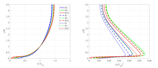
Figure 16.
Mean velocity (left), and TKE (right) profiles for all cases.
As expected, the mean velocity decreases within the forest canopy as the LAI increases. Above the hub height, the mean velocity increases as the forest density increases, as shown in Figure 16 (left). The major feature that is responsible for this behavior is the variation in the aerodynamic drag among trees of the same type with different amounts of foliage. Within and above the canopy, the removal of momentum from the wind flow (which causes less velocity) increases as the aerodynamic drag on the foliage density increases. Meanwhile, above the hub height, the top of the forest canopy serves as a surface for the wind flow where the dense canopies represents a less rough surface compared to the medium sparse and the sparse forest canopies. Thus, the mean velocity behavior above the hub established the fact that the wind speed decreases with increasing surface roughness. Considering different heterogeneity levels of the forest cases, the patched forests have the highest velocity within the canopy and the least above the hub. The homogeneous forest has a higher velocity than the real forest within the canopy, and they behave similarly above the hub.
Comparing the TKE at different heterogeneity levels for respective LAI, Figure 16 (right) shows that above the canopy, for LAI , the homogeneous forests produced the highest TKE, the real forests generated a lower TKE, and the patched forest produced the lowest TKE. A similar observation is made in forests with LAI but with a relatively small difference between the TKE production in homogeneous and real forests. Consequently, as the forest density increases to LAI , the real forest yields a higher TKE production than the homogeneous forests with about increase at the hub height. Meanwhile, among all forest types, the patched forests consistently generate the lowest TKE in the groups even as the density increases. TKE transport is enhanced as the wind acts against the foliage. However, the amount and the morphology of the foliage serves as a mixing layer for TKE production in different forest categories. For instance, in the medium sparse forests, the homogeneous forests act as a balanced permeable layer that allows maximum flow mixing over the forests. Therefore, the lower the heterogeneity level, the higher the TKE level. On the other hand, the trend is different in the case of dense forests (LAI ). Here, the real forest has a higher TKE (by approximately at the hub) than in the homogeneous forest, and it is mainly influenced by the foliage morphology, which allows a better flow mixing over the real forest than the homogeneous forest (somewhat becoming smoother as the density increases).
Generally, TKE is much weaker inside the canopy, with the highest TKE observed in the patched forests. A closer look into the lower ABL shows that within the forest canopy, TKE increases as the LAI decreases for all cases of heterogeneities. However, the ABL interaction with the forest properties above the canopy produces a non-monotonic sequence between TKE production versus LAI, especially in cases of LAI . In all cases, H4 has the highest TKE production followed by R4 and R10, whose TKE profiles merge from . This shows that the real forests behave similarly for LAI ; that is, once the forest LAI reaches up to , the density of the forest has negligible effects on TKE production above the hub height. Further analysis of the relation between forest density and TKE for different heterogeneity levels is presented alongside Figure 17.
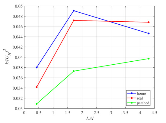
Figure 17.
TKE vs. LAI at hub height for respective heterogeneity cases.
Figure 17 gives the summary of the TKE-LAI relation for forests with different heterogeneity levels. For comparison, the TKE is normalized with the square of the reference velocity. As established by Adedipe et al. [4], where more cases of different forest densities (homogeneous cases) were studied extensively, the TKE increases as the LAI increases until it reaches its maximum TKE production at an average LAI of ; afterwards, it gradually decreases as the forest becomes denser [4]. However, this present study has shown that there is a need to consider the heterogeneity of the forests. Our results support the linear relationship between TKE and forest density with LAI , but the heterogeneity effects in the dense patched forest (strong heterogeneous cases) annul the generalization that the TKE production decreases gradually in denser forests, as the opposite is observed in this case. The results suggest that heterogeneity qualitatively changes the behavior of TKE production in denser forests, and this trend is visible already with the real heterogeneity. In addition, the recent research conducted by Abedi et al. [14], where LES was used to model ABL flow through heterogeneous forests in a wind farm, shows that the homogeneous forest modeling predicted a higher turbulence intensity compared to a heterogeneous forest. However, our current findings show that the inference of Abedi et al. holds only for forest densities with a mean LAI . Therefore, we can conclude that the TKE–LAI relation strongly depends on the heterogeneity of the forest, especially for forest densities with a mean LAI above . We can say that the TKE in different heterogeneity cases depends on the density of the forests, such that as the heterogeneity level increases, the respective TKE increases with increasing LAI. Meanwhile, in the homogeneous (idealized) forests, TKE begins to decrease with increasing LAI after a forest density of LAI is attained. The flow afterwards leads to less tree spacing with no foliage morphology in denser forest, which results in lower TKE production.
5.2. Impacts of Forest Densities on the Wake Flow
This section presents the effects of forest densities on the wake flow of all heterogeneity cases considered in this work. Figure 18 shows the vertical profiles of for different LAIs in respective forest configurations. Generally, the locations are mainly dominated by the turbine rotor effect; hence, the velocity profiles exhibit similar features between different LAI for respective heterogeneity cases. However, significant differences are observed downwind of the turbine as the impact of varying LAI in the wake flow.

Figure 18.
Vertical profiles of velocity deficits (U) from the midplane in different heterogeneous cases with varying densities; (up) homogeneous cases, (middle) real cases, (down) patched cases. The purple shaded region is the turbine rotor area.
It is observed that in the homogeneous forests, presented in Figure 18 (up), H4 has the weakest wake at all locations downstream of the turbine location (). This was consequential to the higher inflow TKE level, which means a higher turbulent mixing (among all cases) leading to a faster flow recovery. This attribute has also been established in both experimental studies and numerical simulations that wind-turbine wakes recover faster in situations of higher turbulence levels in the upstream flow [42,43,44,45]. Meanwhile, H1 and H10 have similar wake profiles, as the absolute error in between the two extreme cases is negligible [4]. A similar trend, as observed in the homogeneous cases, can be seen in the real cases (Figure 18 (middle)), but with a maximum of higher in R1 than observed in R10 at . Figure 18 (down) presents the profiles in the patched forest cases. Here, no significant effects on the wake flow are observed for different LAIs, even though the inflow TKE level shows a linear increase with density. The only remarkable effect in the wake flow of this forest category is observed inside the forest canopy, and this can be accounted for as the effect of the alternating patches in the forest. Overall, changes in the heterogeneity levels are significant on the impacts of different forest densities on the turbine wake-flow.
The profiles of the TKE increase () for different densities are presented for the respective forest cases in Figure 19. A similar order of wake development with varying LAIs is observed between the homogeneous and real forests. Within the rotor area, it is seen that the sparse forests (LAI ) have the highest TKE increase, indicating strong wake effects, which are then followed by the dense forest (LAI ), and then, forests with LAI have the smallest . One major distinction in the wake profiles between homogeneous and heterogeneous forests is that the extreme cases in the homogeneous forest type (H1 and H10) gradually tend toward each other, while the denser forests (R4 and R10, P4 and P10) tends toward each other in the real and patched forests. This feature indicates that as the heterogeneity level of the forests increases, the denser forests exhibit similar flow features in the wake region. On the other hand, the homogeneous forest only shows a trend of similar flow features between the sparse and dense forests.

Figure 19.
Vertical profiles of TKE deficits (k) from the midplane in different heterogeneous cases with varying densities; (up) homogeneous cases, (middle) real cases, (down) patched cases. The purple shaded region is the turbine rotor area.
5.3. Impacts of Varying Heterogeneity Levels on the Wake Flow
The forest cases are further categorized into groups of similar LAIs with the three heterogeneity cases in each group. This helps us to identify the impact of varying heterogeneities in the wake region of forests with similar densities. The profiles for the sparse forests with an average LAI are presented in Figure 20 (up). These sparse forests at different levels of heterogeneity exhibit similar wake behavior downstream of the turbine. The flow features in the wake region are mainly dominated by the large tree spacings and the scarcely distributed foliage in the forests. Thus, we can say that the forest density at this point eliminates the effects of heterogeneity levels in the wake flow.
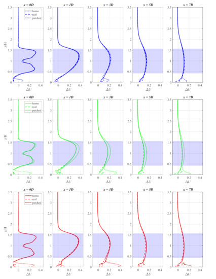
Figure 20.
Vertical profiles of velocity deficits (U) from the midplane for different densities with varying heterogeneity levels. Blue—LAI ; green—LAI ; red—LAI . The purple shaded region is the turbine rotor area.
The medium sparse forest group with mean LAI , presented in Figure 20 (middle), shows a considerable difference between the patched forest and other forest cases with the highest deficit within the rotor area at every location downstream of the turbine. This behavior can be related to the magnitude of the inflow TKE. Considering that the homogeneous and real forests in this group have relatively high inflow TKE compared with that observed over the patched forests, with relatively small variation, this results into a weak and similar wake feature in both cases downstream of the turbine.
The last group, which comprises the dense forests with an average LAI , shows no significant effect of heterogeneity in the wake flow within the rotor area, except at the location, where a minimal detachment is observed in the real forests. This effect can be a result of the natural forest properties at that location, considering the fact that a similar feature is detected at the same location in the medium sparse forests (see Figure 20 (middle)). However, the heterogeneity effect shown in the real forests at the location does not dominate in the sparse forests (see Figure 20 (up)). The reason could be an insufficient amount of foliage for heterogeneity to play any role.
Figure 21 presents the TKE increase () profiles for the corresponding groups shown in the previous figure. The sparse forests (Figure 21 (up)) show a similar order of wake development between the three heterogeneity cases at all locations. The homogeneous forest has the least at all locations downstream of the turbine, followed by the real forest, and the highest is observed in the patched forest, corresponding to the order from the inflow TKE, as shown in Figure 16 (right). It is noteworthy that the flow instability is higher in the homogeneous forest in this group due to the even distribution of uniform sparse trees. In contrast, the flow has less instability over the real and patched forest canopies due to the presence of open spaces and sparse foliage in the forests.
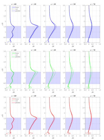
Figure 21.
Vertical profiles of TKE deficits (k) from the midplane for different densities with varying heterogeneity levels. Blue—LAI ; green—LAI ; red—LAI . The purple shaded region is the turbine rotor area.
The medium sparse group is presented in Figure 21 (middle). The patched forest shows a higher magnitude of TKE increase () at all locations compared to other forests. However, the TKE increase () profiles in the homogeneous and real forests merge at all locations, except for a slight difference (about absolute difference) below the hub at the location. With respect to the homogeneous forest, a minimum of approximately higher TKE increase is observed in the patched forest at , while a maximum of increment is observed at .
The dense forest group is presented in Figure 21 (down). Within the rotor area, the real forest show the least deficit, followed by the homogeneous forests, while the highest deficit is found in the patched forest case. With respect to the homogeneous forest, the TKE increase in the patched forest is higher by a maximum of at . However, there is a close relation between the three cases below the hub for further downstream locations (.)
In summary, it can be seen from all three groups that behaves differently below and above the hub. In addition, the deficits peak at at all locations in all cases for all the groups. The patched forests consistently display the highest deficits in all groups, while the homogeneous forests exhibits the least TKE increase in the sparse forests. Additionally, the real forest has the least TKE increase in the dense forests. The medium sparse forest show similar TKE increase in the homogeneous and real forests.
5.4. Wake Development along the Streamwise Direction
Figure 22 shows the wake transition by means of the horizontal profiles of velocity deficit and TKE increase at the hub height downstream of the turbine. Figure 22 (up) shows a similar wake-development behavior along the stream-wise direction. In all cases, the peak of the velocity deficits is observed at about from the turbine, while the flow recovers gradually in a similar manner downstream. Altogether, the medium sparse forest in the homogeneous and real forests exhibit faster wake recovery among all cases. In Figure 22 (down), substantial differences are observed in the plots between ; afterwards, the differences gradually diminish toward the outlet. Overall, the medium sparse forests (LAI ) for homogeneous and real forests have the shortest wake. The strength of the wake in the rest of the cases differs with density and/or heterogeneity at different locations.

Figure 22.
Wake transition of the velocity deficit () (up) and TKE increase () (down) taken from the horizontal line at the hub height.
Furthermore, Figure 23 and Figure 24 help to qualitatively compare the modeled turbine-generated turbulence and velocity in different cases. It can be seen that the flow recovery behaves similarly in all cases except in the patched forest (strong heterogeneous cases) where a wavy feature is exhibited, which is due to the alternating small patches present in the forest configuration. The wakes of a stand-alone wind turbine typically exhibit an axisymmetric shape with the peak around the hub height. The wake is explained to be the influence of the forest characteristics, which not only causes increased turbulent mixing but affect the wake behavior in terms of its length and width in the wake region. In our study, this feature is more pronounced in the homogeneous cases and the sparse forests of the heterogeneous cases. Meanwhile, the denser the forest, the higher the peak in the real forests, and the wider the width of the peak (span-wise) in the strong heterogeneous forests.
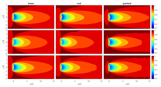
Figure 23.
Mean velocity contours from horizontal (X-Y) planes at the hub height. Row-wise, LAI .
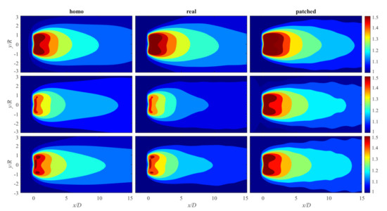
Figure 24.
Mean TKE contours from horizontal (X-Y) planes at the hub height. Row-wise, LAI .
6. Conclusions
The paper presents a detailed study on the numerical simulations of the wind-turbine wake over three different forest heterogeneities. A total of nine forest cases are simulated to achieve the aim of this study. The forest cases are with LAI values of , and for homogeneous, real, and patched forests, respectively. The numerical set-up is designed such that the ABL flow is fully developed over respective forests before its interaction with the turbine. The Unsteady-RANS technique is employed using OpenFOAM. The NREL 5 MW virtual wind turbine is used, while the ALM theory is applied to model the wake turbine effects in the simulations [25].
Our findings show that the upstream TKE level over forests of different densities (LAI) strongly depends on the heterogeneity of the forest, especially for forest densities with a mean LAI above . Before the turbine, the homogeneous forest is seen to have higher TKE compared to the heterogeneous forests (real and patched) for LAI less than approximately 2. The heterogeneity effects in the real and patched forests lead to an increase in the upstream TKE in the case of denser forests (LAI = ).
These results further suggest that the effect any forest can have on a stand-alone wind turbine largely depends on the density and the heterogeneity of the forest. Our analyses show that alteration in the heterogeneous nature of the forests changes the impact of density in the wake behavior and vice versa. Increasing forest density in heterogeneous forests causes higher upstream TKE, which eventually leads to a shorter wake downstream of the turbine. On the other hand, the homogeneous forest varies non-monotonically with forest density. The upstream TKE increases as the density increases, reaches its maximum at an average LAI of , and then decreases slowly as the density increases. This also leads to shorter wake downstream of the turbine in forests with LAI , while the wake in lesser and denser forests behaves similarly.
The turbulent flow characteristics over forest canopies become more evident as the canopy density increases, with emphasis that the forest is heterogeneous either naturally or ideally. The conclusion does not hold for a uniform, ideal, homogeneous forests, especially with an LAI [4].
In conclusion, the results from this research can help the wind-energy industry and researchers to enable the optimization of turbines, better operations, and maintenance in forested wind farms. However, the methodology used in this present work is limited due to the implementation of RANS. A more detailed analysis of turbulence characteristics in different forest heterogeneities with the inclusion of wind turbines can be obtained with LES. A possible extension of this work in the near future includes the analysis of the results in association with turbine loads with LES techniques. Real terrain data could also be incorporated with the real forest data for an extensive study on the impacts of real forested terrain on wind turbines.
Author Contributions
Conceptualization, T.A., A.C. and A.H.; Data curation, T.K.; Funding acquisition, H.H.; Investigation, T.A. and A.C.; Methodology, T.A. and A.C.; Resources, H.H.; Supervision, A.C. and A.H.; Validation, T.A. and A.C.; Visualization, T.A.; Writing—original draft, T.A.; Writing—review and editing, T.A. All authors have read and agreed to the published version of the manuscript.
Funding
This work was supported by the Academy of Finland, decision number 313827, ‘Industrial Internet and Data Analysis in Marine Industries’, and by the Centre of Excellence of Inverse Modelling and Imaging (CoE), Academy of Finland, decision number 312 125.
Acknowledgments
The authors gratefully acknowledge the financial aid from the department of Computational Engineering, School of Engineering Science, Lappeenranta-Lahti University of Technology, Finland. We also appreciate the CSC-IT Center for Science, Finland on whose platform the computations in this project were performed. Finally, the effort of all reviewers of this manuscript is well appreciated.
Conflicts of Interest
The authors declare no conflict of interest.
References
- Nebenführ, B.; Davidson, L. Prediction of wind-turbine fatigue loads in forest regions based on turbulent LES inflow fields. Wind Energy 2017, 20, 1003–1015. [Google Scholar] [CrossRef]
- Desmond, C.J.; Watson, S.J.; Aubrun, S.; Ávila, S.; Hancock, P.; Sayer, A. A study on the inclusion of forest canopy morphology data in numerical simulations for the purpose of wind resource assessment. J. Wind. Eng. Ind. Aerodyn. 2014, 126, 24–37. [Google Scholar] [CrossRef] [Green Version]
- Chaudhari, A.; Agafonova, O.; Hellsten, A.; Sorvari, J. Numerical Study of the Impact of Atmospheric Stratification on a Wind-Turbine Performance. J. Phys. Conf. Ser. 2017, 854, 11. [Google Scholar] [CrossRef] [Green Version]
- Adedipe, T.A.; Chaudhari, A.; Kauranne, T. Impact of different forest densities on atmospheric boundary-layer development and wind-turbine wake. Wind Energy 2020, 23, 1165–1180. [Google Scholar] [CrossRef]
- Hefny Salim, M.; Heinke Schlünzen, K.; Grawe, D. Including trees in the numerical simulations of the wind flow in urban areas: Should we care? J. Wind. Eng. Ind. Aerodyn. 2015, 144, 84–95. [Google Scholar] [CrossRef] [Green Version]
- Shaw, R.H.; Schumann, U. Large-eddy simulation of turbulent flow above and within a forest. Bound.-Layer Meteorol. 1992, 61, 47–64. [Google Scholar] [CrossRef] [Green Version]
- Chaudhari, A.; Conan, B.; Aubrun, S.; Hellsten, A. Numerical study of how stable stratification affects turbulence instabilities above a forest cover: Application to wind energy. J. Phys. Conf. Ser. 2016, 753, 1–12. [Google Scholar] [CrossRef] [Green Version]
- Agafonova, O.; Avramenko, A.; Chaudhari, A.; Hellsten, A. The effects of the canopy created velocity inflection in the wake development. AIP Conf. Proc. 2016, 1738, 480082. [Google Scholar] [CrossRef]
- Dwyer, M.J.; Patton, E.G.; Shaw, R.H. Turbulent kinetic energy budgets from a large-eddy simulation of airflow above and within a forest canopy. Bound.-Layer Meteorol. 1997, 84, 23–43. [Google Scholar] [CrossRef]
- Dalpé, B.; Masson, C. Numerical study of fully developed turbulent flow within and above a dense forest. Wind Energy 2008, 11, 503–515. [Google Scholar] [CrossRef]
- Étienne Boudreault, L.; Bechmann, A.; Tarvainen, L.; Klemedtsson, L.; Shendryk, I.; Dellwik, E. A LiDAR method of canopy structure retrieval for wind modeling of heterogeneous forests. Agric. For. Meteorol. 2015, 201, 86–97. [Google Scholar] [CrossRef] [Green Version]
- da Costa, J.L.; Castro, F.; Palma, J.; Stuart, P. Computer simulation of atmospheric flows over real forests for wind energy resource evaluation. J. Wind. Eng. Ind. Aerodyn. 2006, 94, 603–620. [Google Scholar] [CrossRef]
- Monsi, M.; Saeki, T. On the Factor Light in Plant Communities and its Importance for Matter Production. Ann. Bot. 2005, 95, 549–567. [Google Scholar] [CrossRef] [PubMed] [Green Version]
- Abedi, H.; Sarkar, S.; Johansson, H. Numerical modelling of neutral atmospheric boundary layer flow through heterogeneous forest canopies in complex terrain (a case study of a Swedish wind farm). Renew. Energy 2021, 180, 806–828. [Google Scholar] [CrossRef]
- Bergström, H.; Alfredsson, H.; Arnqvist, J.; Carlén, I.; Dellwik, E.; Fransson, J.; Ganander, H.; Mohr, M.; Segalini, A.; Söderberg, S. Wind Power in Forests: Wind and Effects on Loads; Technical Report Elforsk AB; Technical University of Denmark (DTU): Stocholm, Sweden, 2013. [Google Scholar]
- Wu, Y.T.; Porté-Agel, F. Atmospheric turbulence effects on wind-turbine wakes: An LES study. Energies 2012, 5, 5340–5362. [Google Scholar] [CrossRef]
- Desmond, C.; Watson, S.; Montavon, C.; Murphy, J. Modelling uncertainty in t-RANS simulations of thermally stratified forest canopy flows for wind energy studies. Energies 2018, 11, 1703. [Google Scholar] [CrossRef] [Green Version]
- Dalpé, B.; Masson, C. Numerical simulation of wind flow near a forest edge. J. Wind. Eng. Ind. Aerodyn. 2009, 97, 228–241. [Google Scholar] [CrossRef]
- Laan, M.; Sørensen, N.N.; Réthoré, P.E.; Mann, J.; Kelly, M.; Troldborg, N.; Schepers, J.; Machefaux, E. An improved k-ϵ model applied to a wind turbine wake in atmospheric turbulence. Wind Energy 2015, 18, 889–907. [Google Scholar] [CrossRef] [Green Version]
- Gómez-Elvira, R.; Crespo, A.; Migoya, E.; Manuel, F.; Hernández, J. Anisotropy of turbulence in wind turbine wakes. J. Wind. Eng. Ind. Aerodyn. 2005, 93, 797–814. [Google Scholar] [CrossRef]
- Kasmi, A.E.; Masson, C. An extended k–ϵ model for turbulent flow through horizontal-axis wind turbines. J. Wind. Eng. Ind. Aerodyn. 2008, 96, 103–122. [Google Scholar] [CrossRef]
- Erek, k-ϵ Turbulence Modeling for a Wind Turbine: Comparison of RANS Simulations with ECN Wind Turbine Test Site Wieringermeer (EWTW) Measurements. 2011. Available online: http://www.diva-portal.org/smash/get/diva2:586991/FULLTEXT01.pdf (accessed on 14 January 2022).
- Weller, H.G.; Tabor, G.; Jasak, H.; Fureby, C. A tensorial approach to computational continuum mechanics using object-oriented techniques. Comput. Phys. 1998, 12, 620–631. [Google Scholar] [CrossRef]
- Jonkman, J.; Butterfield, S.; Musial, W.; Scott, G. Definition of a 5-MW Reference Wind Turbine for Offshore System Development; Technical Report NREL/TP-500-38060; National Renewable Energy Lab. (NREL): Golden, CO, USA, 2009. [Google Scholar]
- Sørensen, J.; Shen, W. Numerical modeling of wind turbine wakes. J. Fluids Eng. 2002, 124, 393–399. [Google Scholar] [CrossRef]
- Arnqvist, J.; Segalini, A.; Dellwik, E.; Bergström, H. Wind Statistics from a Forested Landscape. Bound.-Layer Meteorol. 2015, 156, 53–71. [Google Scholar] [CrossRef]
- Nebenführ, B.; Davidson, L. Large-Eddy Simulation Study of Thermally Stratified Canopy Flow. Bound.-Layer Meteorol. 2015, 156, 253–276. [Google Scholar] [CrossRef] [Green Version]
- Nebenführ, B.D.L. Influence of a forest canopy on the neutral atmospheric boudary layer-A LES study. In Proceedings of the 10th International ERCOFTAC Symposium on Turbulence Modelling and Measurements, Marbella, Spain, 17–19 September 2014. [Google Scholar]
- Garrigues, S.; Allard, D.; Baret, F.; Weiss, M. Quantifying spatial heterogeneity at the landscape scale using variogram models. Remote Sens. Environ. 2006, 103, 81–96. [Google Scholar] [CrossRef]
- Shih, T.H.; Liou, W.W.; Shabbir, A.; Yang, Z.; Zhu, J. A new k-ϵ eddy viscosity model for high reynolds number turbulent flows. Comput. Fluids 1995, 24, 227–238. [Google Scholar] [CrossRef]
- Schmitz, S.; Jha, P. Modeling the Wakes of Wind Turbines and Rotorcraft Using the Actuator-Line Method in an OpenFOAM -LES Solver. 2013. Available online: https://pennstate.pure.elsevier.com/en/publications/modeling-the-wakes-of-wind-turbines-and-rotorcraft-using-the-actu (accessed on 14 January 2022).
- Dağ, K.O.; Sørensen, J.N. A new tip correction for actuator line computations. Wind Energy 2020, 23, 148–160. [Google Scholar] [CrossRef]
- Agafonova, O. A Numerical Study of Forest Influences on the Atmospheric Boundary Layer and Wind Turbines. Ph.D.Thesis, Lappeenranta University of Technology, Lahti, Finland, 2017. [Google Scholar]
- Troldborg, N. Actuator Line Modeling of Wind Turbine Wakes. Ph.D. Thesis, Technical University of Denmark, Copenhagen, Denmark, 2009. [Google Scholar]
- Glauert, H. Airplane propellers. In Aerodynamic Theory; Durand, W.F., Ed.; Dover: New York, NY, USA, 1963; pp. 169–360. [Google Scholar]
- Mendoza, V.; Chaudhari, A.; Goude, A. Performance and wake comparison of horizontal and vertical axis wind turbines under varying surface roughness conditions. Wind Energy 2019, 22, 458–472. [Google Scholar] [CrossRef]
- Baba-Ahmadi, M.; Tabor, G. Inlet conditions for LES using mapping and feedback control. Comput. Fluids 2009, 38, 1299–1311. [Google Scholar] [CrossRef] [Green Version]
- Chaudhari, A.; Vuorinen, V.; Agafonova, O.; Hellsten, A.; Hämäläinen, J. Large-eddy simulation for atmospheric boundary layer flows over complex terrains with applications in wind energy. In Proceedings of the 11th World Congress on Computational Mechanics, Barcelona, Spain, 20–25 July 2014; pp. 5205–5216. [Google Scholar]
- Chaudhari, A.; Vuorinen, V.; Hämäläinen, J.; Hellsten, A. Large-eddy simulations for hill terrains: Validation with wind-tunnel and field measurements. Comput. Appl. Math. 2018, 37, 2017–2038. [Google Scholar] [CrossRef]
- Chaudhari, A.; Hellsten, A.; Hämäläinen, J. Full-Scale Experimental Validation of Large-Eddy Simulation of Wind Flows over Complex Terrain: The Bolund Hill. Adv. Meteorol. 2016, 2016, 9232759. [Google Scholar] [CrossRef] [Green Version]
- Su, H.B.; Shaw, R.H.; Paw, U.K.T. Two-Point Correlation Analysis Of Neutrally Stratified Flow Within And Above A Forest From Large-Eddy Simulation. Bound.-Layer Meteorol. 2000, 94, 423–460. [Google Scholar] [CrossRef]
- Chamorro, L.P.; Porté-Agel, F. A Wind-Tunnel Investigation of Wind-Turbine Wakes: Boundary-Layer Turbulence Effects. Bound.-Layer Meteorol. 2009, 132, 129–149. [Google Scholar] [CrossRef] [Green Version]
- Zhang, W.; Markfort, C.D.; Porté-Agel, F. Near-wake flow structure downwind of a wind turbine in a turbulent boundary layer. Exp. Fluids 2012, 52, 1219–1235. [Google Scholar] [CrossRef] [Green Version]
- Rados, K.; Larsen, G.; Barthelmie, R.; Schlez, W.; Lange, B.; Schepers, G.; Hegberg, T.; Magnisson, M. Comparison of Wake Models with Data for Offshore Windfarms. Wind Eng. 2001, 25, 271–280. [Google Scholar] [CrossRef] [Green Version]
- Cheng, S.; Elgendi, M.; Lu, F.; Chamorro, L.P. On the Wind Turbine Wake and Forest Terrain Interaction. Energies 2021, 14, 7204. [Google Scholar] [CrossRef]
Publisher’s Note: MDPI stays neutral with regard to jurisdictional claims in published maps and institutional affiliations. |
© 2022 by the authors. Licensee MDPI, Basel, Switzerland. This article is an open access article distributed under the terms and conditions of the Creative Commons Attribution (CC BY) license (https://creativecommons.org/licenses/by/4.0/).