A Horse Herd Optimization Algorithm (HOA)-Based MPPT Technique under Partial and Complex Partial Shading Conditions

Abstract

The inconsistent irradiance, temperature, and unexpected behavior of the weather affect the output of photovoltaic (PV) systems, classified as partial or complex partial shading conditions. Under these circumstances, obtaining the maximum output power from PV systems becomes problematic. This paper proposes a population-based optimization model, the horse herd optimization algorithm (HOA), inspired by natural behavior, to solicit the maximum power under partial or complex partial shading conditions. It is an intelligent strategy inspired by the surprise pounce-chasing style of the horse herd model. The proposed technique outperforms the standard in different weather conditions, needs less computational time, and has a fast convergence speed and zero oscillations after reaching a power point’s maximum limit. A performance comparison of the HOA is achieved with conventional techniques, such as “perturb and observe” (P&O), the bio-inspired adaptive cuckoo search optimization (ACS), particle swarm optimization (PSO), and the dragonfly algorithm (DA). The following comparison of the presented scheme with the other techniques shows its better performance with respect to fast tracking and efficiency, as well as stability under disparate weather conditions and the ability to obtain maximum power with negligible oscillation under partial and complex shading.

1. Introduction

As stated by the International Energy Agency (IEA), about 28% of worldwide electricity generation in 2020 is based on renewable energy, and 90% of the new installed power capacity is generated using renewable sources [1]. Photovoltaic (PV) generated power capacity has increased by a factor of 18 since 2010. The most significant parameters of PV systems are their ease of availability, low maintenance cost, eco-friendly production, and the system’s renewable nature. PV systems may be used as either grid-connected or standalone alternative energy sources [2]. A maximum power point (MPP) searching technique is critical in order to achieve the efficient operation of any PV system, which enables the maximum conversion of solar energy to power. The MPPT performance in PV energy systems is compromised due to the various shading conditions of PV panels; these shading conditions can be classified into partial and complex partial shading. In the literature, various works are available that deal with optimization techniques to mitigate these shading conditions [3,4]. Therefore, advanced PV systems are proposed in the literature, and a block diagram of such a system is shown in Figure 1 that includes sensors for voltage and current measurement and a DC-DC Cuk converter, using the MPPT technique, which, in turn, controls the Cuk converter and drives the switch for the DC-DC converter [5].

In this article, we focus on an optimization technique for the efficient operation of a PV system in partial shading (PS) and complex partial shading (CPS) conditions. Therefore, we will now briefly discuss recent works relevant to this field.

1.1. Prior Works

Regarding the current-voltage and power-voltage characteristics of PV, the characteristics curves of the power-voltage (P-V) and current-voltage (I-V) of photovoltaic cells are non-linear, due to changes in weather conditions. However, to deal with nonlinearities, the MPP technique is employed to predict and harvest the MPP in rapidly changing and variable weather conditions and also to optimize the system to run at MPP. Many conventional, as well as soft-computing, MPPT algorithms have been introduced to upgrade the effectiveness of photovoltaic energy systems through PS and uniform irradiance (UI) conditions. Several techniques are suggested in the published literature that deals with uniform irradiance to achieve MPPT, while more recent research works refer to optimization techniques that are applied for PS conditions [5], although few discuss CPS conditions.

Some of the classical techniques for MPPT in PV systems are briefly discussed here. The fractional short circuit current (FSCC) technique makes it quick and simple to harvest the maximum power point, although the drawback is that it cannot track the exact MPP and works in offline mode [5]. The fractional open-circuit voltage (FOCV) technique is a direct, simple, offline, and easy to implement technique similar to FSCC; however, it is unable to track the exact MPP [5]. Similarly, “perturb and observe” (P&O) is an extensively exploited technique for the finding of MPP. Its working technique is the same as that in hill-climbing algorithms, and it is able to track the MPP in both offline and online modes, but its performance decreases when a PS condition occurs [5]. Incremental conductance (InC) performs better than P&O; however, it does not extract the exact MPP. It also works on the principle of the hill-climbing algorithm [6].

The classical techniques are simple and have a very fast response time; however, these techniques are not effective for attaining global maxima (GM) in the online mode and for dynamically changing PS conditions. Therefore, to achieve MPP in non-uniform environmental conditions, many soft computing techniques have been introduced in the literature. Several of these are based on fuzzy logic and artificial intelligence [7]. Hybrid techniques can be used in combination with other techniques like InC and P&O, in order to improve the system’s efficiency under PS conditions [8]. In [9], the author presents a new MPPT control for PV systems that depends on the search and rescue (SRA) optimization method. The suggested approach improves PV system efficiency by decreasing the oscillations at the global maximum (GM) and monitoring the GM quickly and efficiently. Other notable aspects of the proposed SRA control technique include robustness, power tracking performance in a steady state, and implementation simplicity. Many evolutionary algorithms, such as the particle swarm optimization (PSO) algorithm, the genetic method (GA), etc., are stochastically based methods that are efficient for optimization. However, these are unable to track MPP under CPS and give optimal performance, in terms of convergence and tracking speed, to harvest GM. Adaptive cuckoo optimization (ACO) is another technique that is inspired by an animal model, the aggressive reproduction behavior of the cuckoo. ACO gives improved performance, has good convergence speed and approximate accuracy, and requires a smaller number of parameters for tuning, although it is unable to track MPP under CPS conditions [10,11].

In [12], the authors present a paper using an HOA with a boost converter and battery load installed within the PV system. When the battery load provides a constant voltage, the boost converter performs better, but in a grid-tied PV system, where battery load is not installed as part of the PV system, the boost converter is unable to provide the desired performance. In the grid-tied PV system, the output fluctuates because the boost converter cannot provide a constant voltage, because of which the performance of the PV system deteriorates; therefore, a bidirectional Cuk converter is used in the current research work. A Cuk converter is used to overcome output fluctuations when the PV system is grid-tied (without a battery load) in combination with an intelligent technique, which can harvest GM under PS and CPS conditions.

1.2. Contribution

In this article, we propose the application of the horse herd optimization algorithm (HOA) method, which is a nature-inspired technique with the characteristic of harvesting energy under PS and CPS conditions. The performance of the HOA is evaluated in terms of various parameters, such as settling time, convergence speed, and fewer iterations to find the GM. Furthermore, an intensive comparison of the HOA is presented that can track the maximum energy under PS and CPS conditions. The HOA is tested in terms of different scenarios for PS and CSP, and its performance is compared with that of other optimization techniques.

The motivation for utilizing HOA for MPPT in PS and CPS is due to a number of factors. These include fewer iterations while tracking GM, with close to zero oscillations, an almost 100% tracking efficiency, the lowest settling time, and its efficiency in terms of tracking speed in addition to a steady-state response with the bidirectional Cuk converter. The structure of the Cuk converter is that of a boost converter, involving a buck converter as well. It converts one voltage level to another voltage level, having zero-ripple current. It can produce either step-up or -down voltages, a property that makes its use desirable for a wide range of voltage applications. In the majority of prior works, boost converters and battery loads are used. Boost converters perform better when a battery load is installed with the PV system since batteries provide a constant output voltage; however, when battery load is not installed with the PV system, the output voltage fluctuates. The main motivation here for using the Cuk converter is that it exhibits both the properties of step-down and step-up voltages and gives a continuous output, even when no battery load is installed with a PV system.

The design of the Cuk converter allows a continuous current flow through the input side, regardless of the state of the switch. The circuit in Figure 2 depicts a Cuk converter, which shows that the application of LC filters at the input and output sides facilitates a smooth current waveform.

The Cuk converter also produces a very low output voltage ripple, due to the presence of a second-order low-pass filter. This filter is a combination of inductors and capacitors found in the converter. The design of the inductor ensures zero-ripple behaviour and a reduction in electromagnetic interference. Therefore, the overall impact of this converter’s utilization is inherently low noise and the greater efficiency of the PV energy system.

The analysis in this article is carried out in the context of HOA applications and highlights the following contributions.

Under different weather circumstances, the performance of the chosen approach is contrasted to that of some other techniques.

• Its superiority is underlined by the experimental results and, since only one parameter is used for the exploration and exploitation phase it results, in terms of quick tracking, in almost zero oscillations.
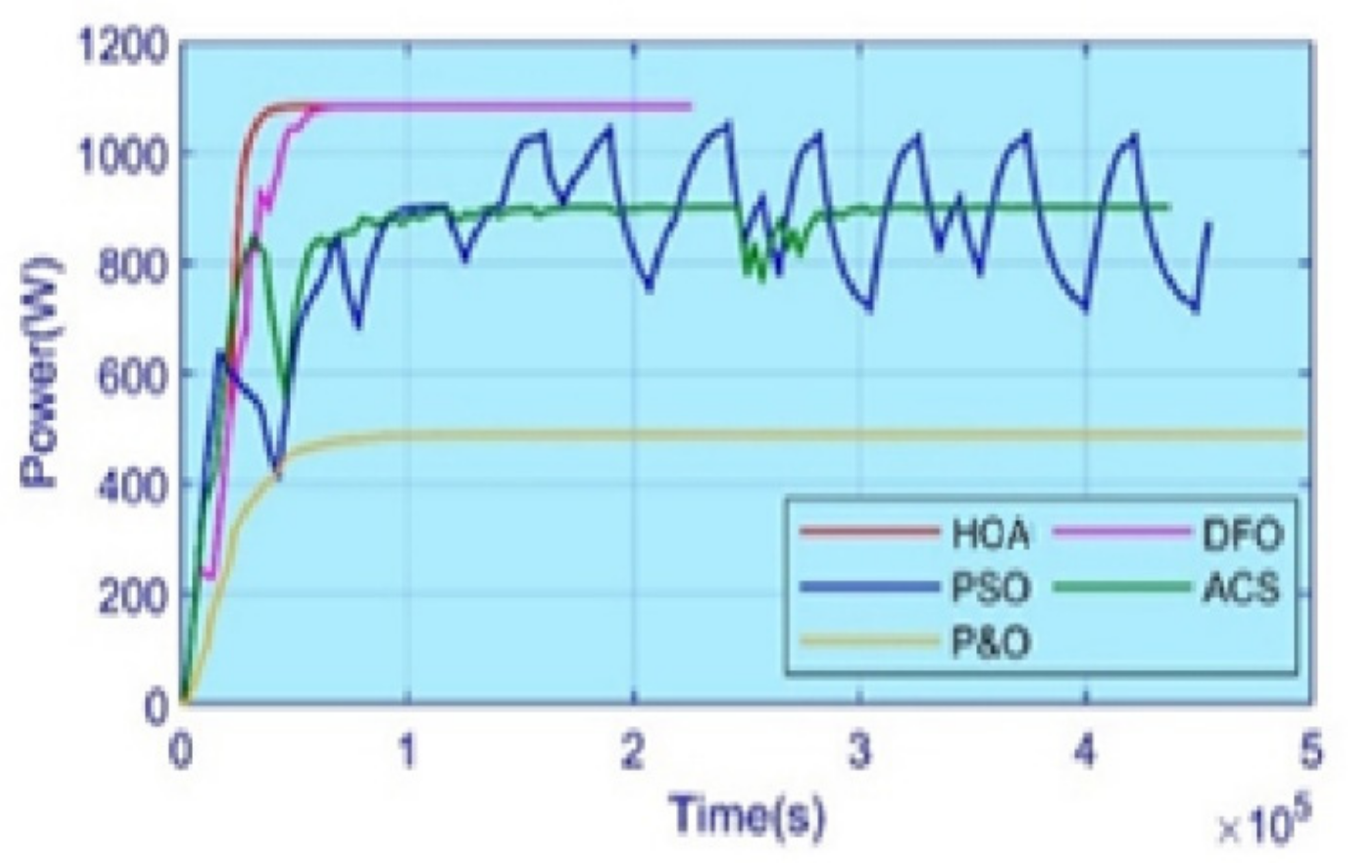
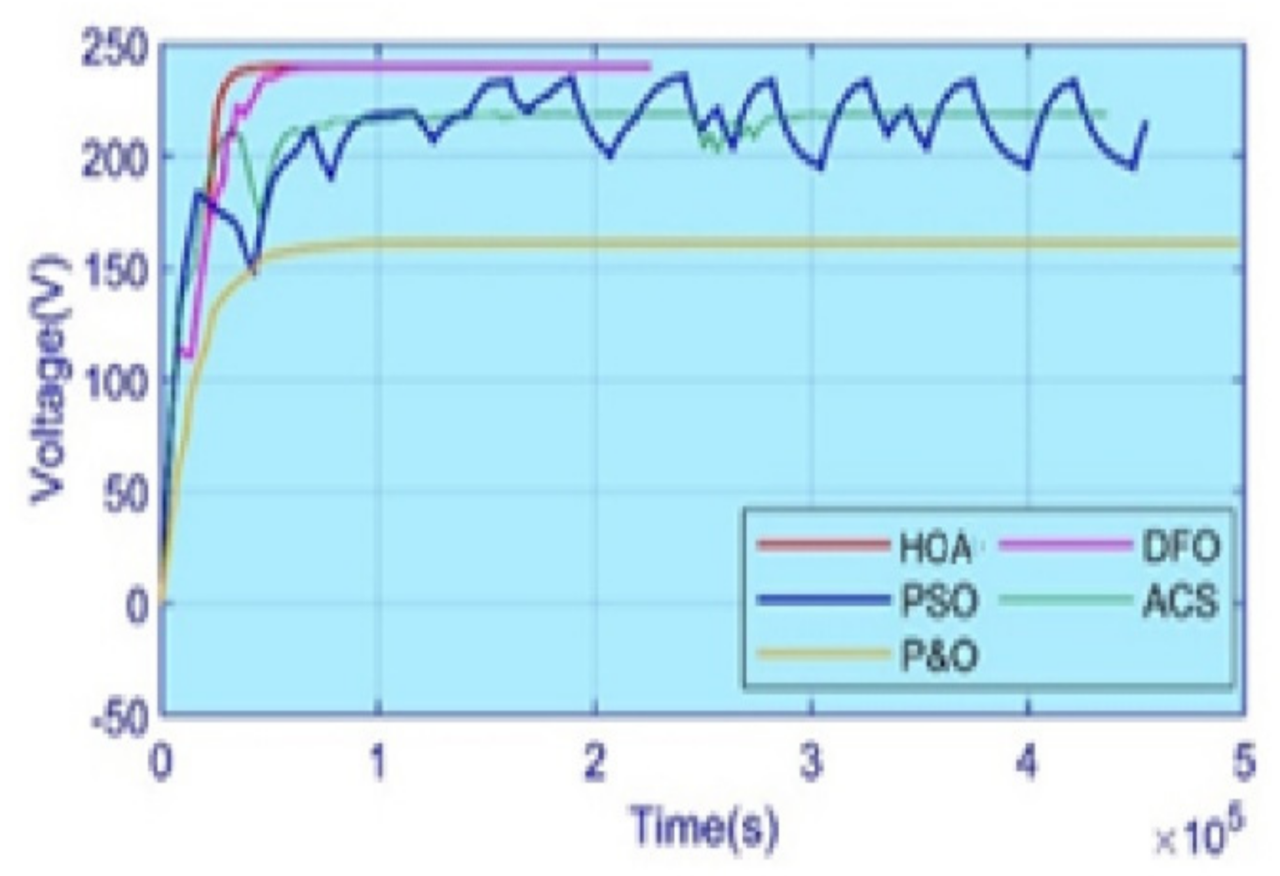
• The HOA particles are able to remain stationary and the oscillation becomes equal to zero when a cycle of iteration ends, and the power converging efficiency is approximately 99.1%. The absence of this characteristic in PSO and ACS, etc. results in the loss of power and unwanted oscillations.
• The comparison between the HOA and the existing scheme is performed under four different scenarios of weather conditions. The HOA technique can harvest maximum energy under PS and CPS. Moreover, the results of tracking the MPP under different PS and CPS scenarios are represented in the experimental part of this paper, which clearly shows that the HOA technique performs better with respect to convergence rate and zero oscillation, as well as fast-tracking in comparison to P&O, InC, PSO, ACS, and DFO. The HOA technique does not oscillate on GM and will successfully reach a steady state, resulting in the increase in efficiency of the overall system.

1.3. Organization

This paper comprises the following sections. The PS and CPS are discussed in Section 2. Section 3 and Section 4 present the mathematical model and the tracking mechanism of the HOA algorithm, respectively. A detailed comparative analysis of the HOA algorithm with the other optimization algorithms is illustrated in Section 5. Finally, our conclusions are presented in Section 6.

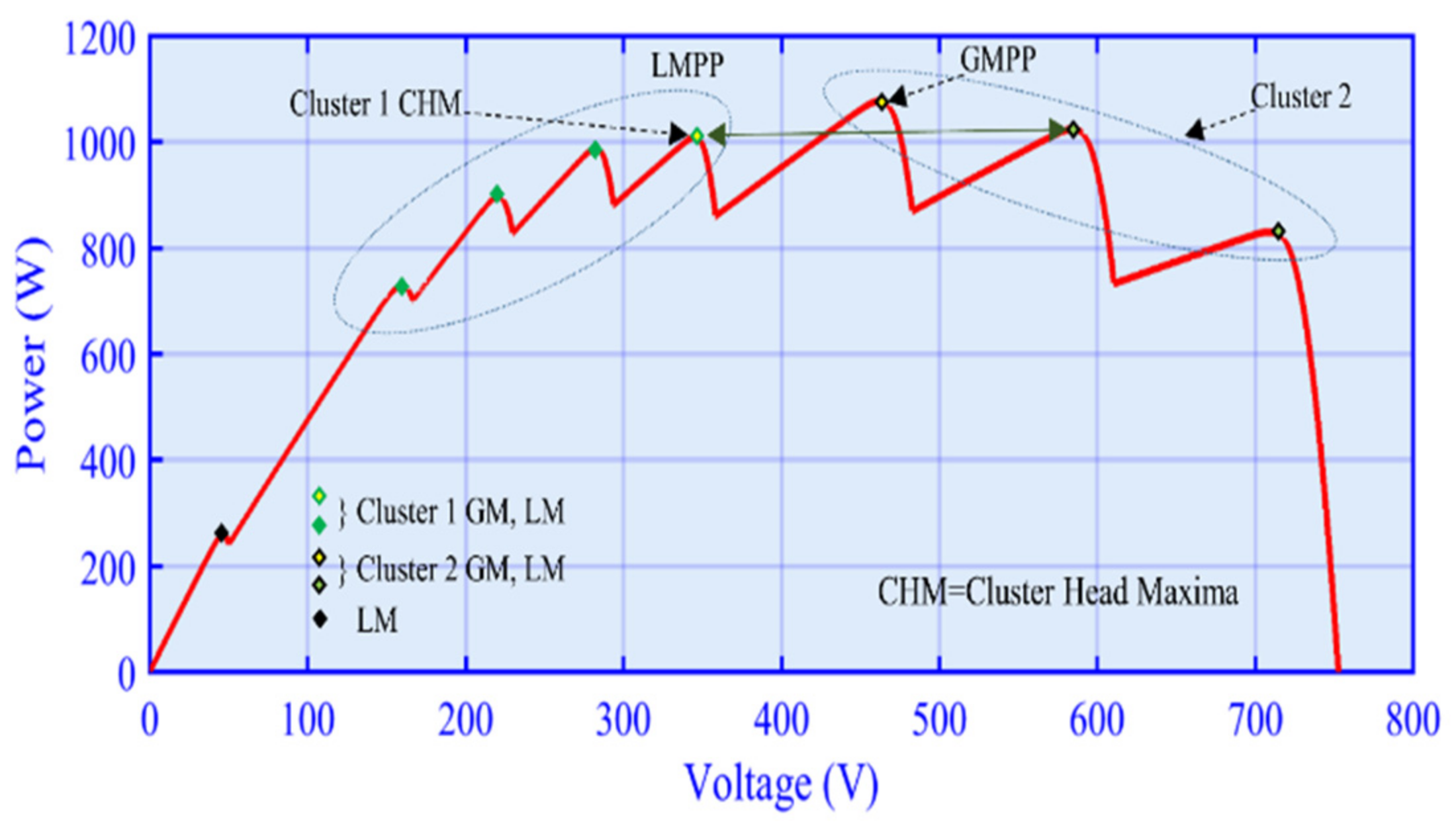
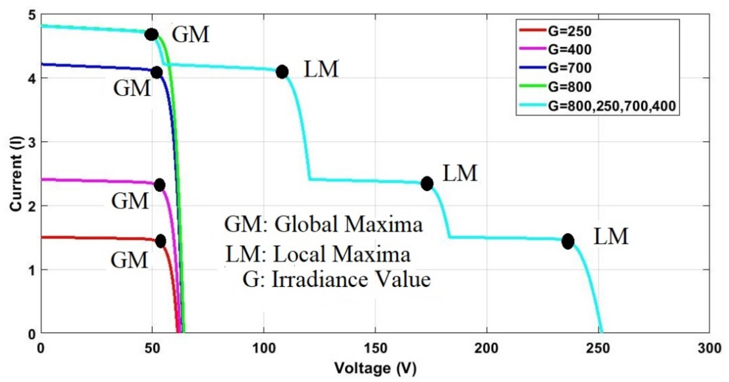
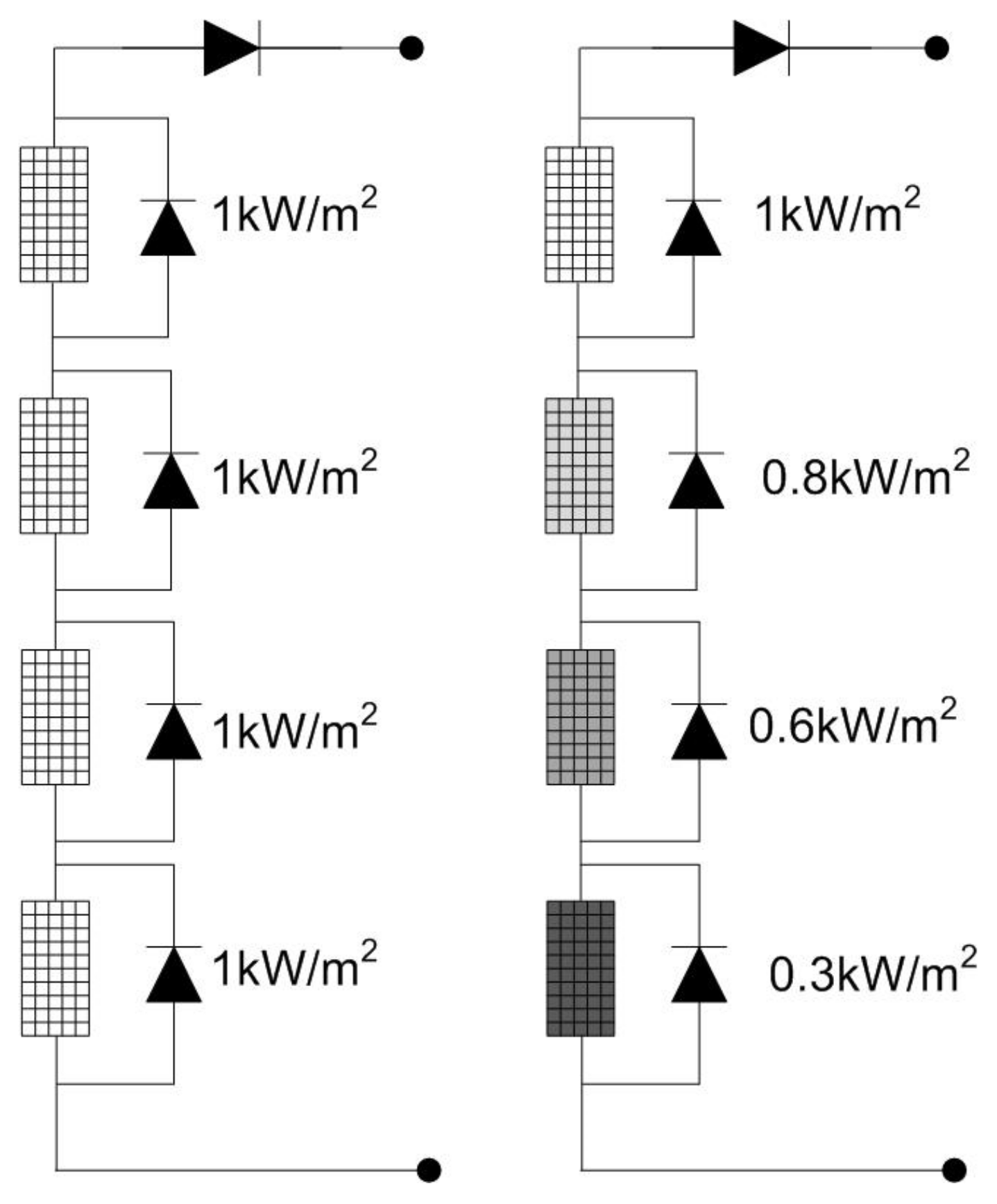
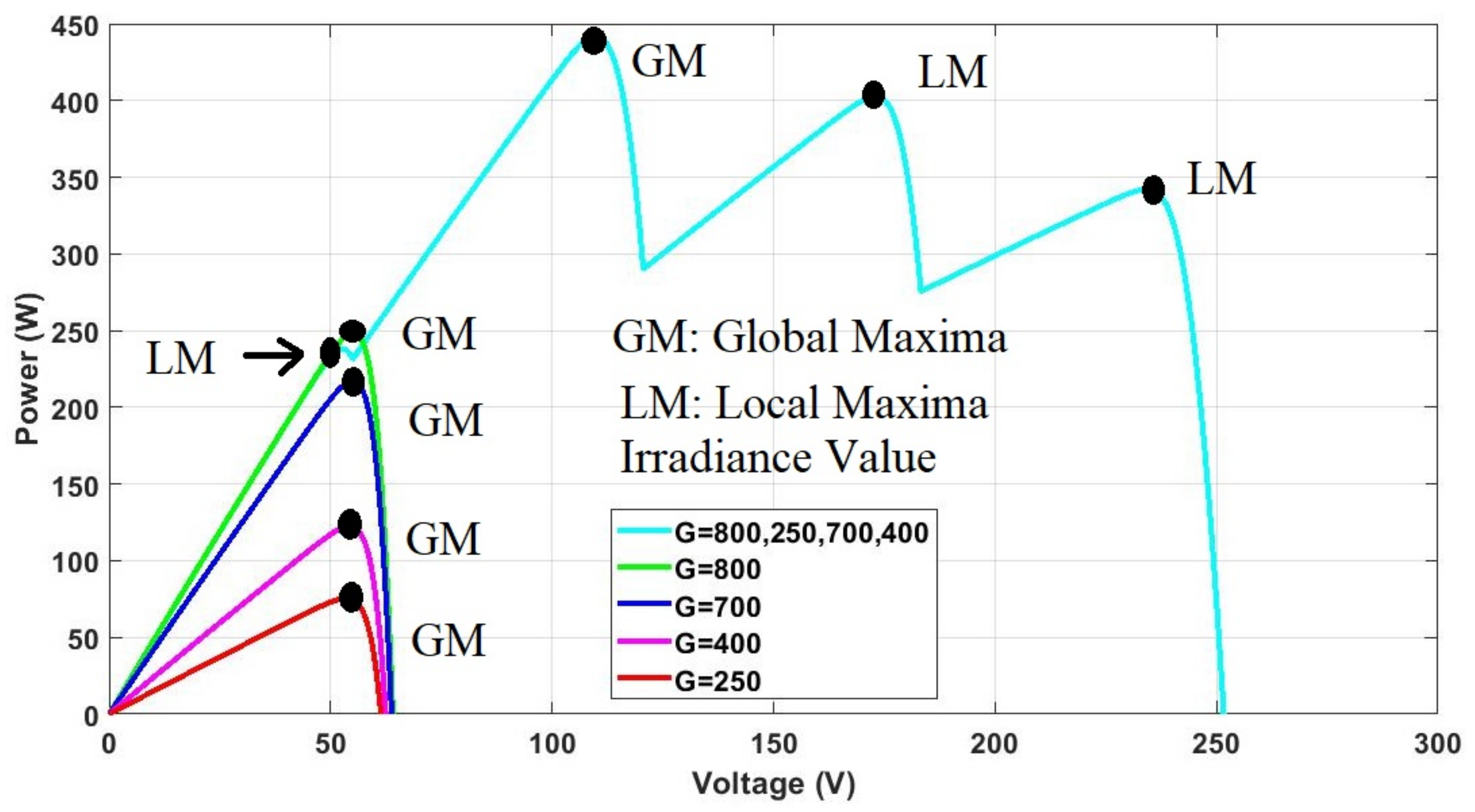
2. Partial and Complex Partial Shade

When one portion of the PV module receives an inconsistent irradiance that is different from the rest of the PV area, the PV system fails to provide a uniform output; as a result, PS or, in the worst-case scenario, CPS occurs. Under these conditions, whether PS or CPS, different irradiance levels are received by the PV modules [13].

The shaded modules are unable to provide the desired voltage, degrading its efficiency, and as a result, mismatching effects occur. To counter a bypass diode, the mismatching effects can be reduced [14]. Figure 3 shows a set of four PV modules, joined in a series, with a bypass diode in the reverse direction. In uniform irradiance conditions, all diodes receive an equal amount of irradiance, $1000 \mathrm{W}/{\mathrm{m}}^2,$ and there is no drop in voltage. Under PS conditions, PV modules receive various levels of irradiance, which are $1000 \mathrm{W}/{\mathrm{m}}^2$,$600 \mathrm{W}/{\mathrm{m}}^2$,$300 \mathrm{W}/{\mathrm{m}}^2$,$\mathrm{and} 800 \mathrm{W}/{\mathrm{m}}^2,$ as shown in Figure 3. The P-V curves are demonstrated in Figure 4 and Figure 5, and Figure 6 shows the UIC, PS, and CPS conditions.

PV modules are connected in series, and, in PS conditions, each module has an effect on the PV system. Figure 7 shows the IV curve of the PV system. There are four PV modules used for PS scenarios. PV modules 1, 2, 3, and 4 have irradiance (G) values of 800, 250, 700, and 400, respectively, and their currents are 1.6 A, 2.4 A, 4.2 A, and 4.8 A, respectively. The individual modules have only single global maxima (GM). However, when combinations of four PV modules are used, a single GM and three local maxima (LM) appear on the IV curves.

Figure 8 illustrates the power voltage curves of the PV system. Each PV module has its own power rating. Individually, PV modules 1, 2, 3, and 4 give a power of 70 W, 120 W, 220 W, and 250 W, respectively. Moreover, in the case of a combination of four PV modules, only one GM and three LM appear on the PV curve. When all the PC modules are connected in series, they give a power of 449.8 W at the GM.

3. Mathematical Model of the HOA Algorithm

The behavioral patterns of horses in their natural habitat are the basis for this study. The grazing, hierarchy, sociability, imitation, defense mechanism, and roaming behaviors are the most common behavioral patterns seen in horses [15]. As a result, the six general behaviors of horses of various ages provide the inspiration for this method. At each step, the horses are moved in accordance with Equation (1).

$$P_m^{iter,age}=Ve{l}_m^{iter,age}+P_m^{\left(iter-1\right),age}, age=\alpha , \beta , \gamma , \delta$$

(1)

In this equation:

• $P_m^{iter,age}$ denotes the $mth$ horse position.
• $age$ shows the range of each horse.
• $iter$ describes the current number of iterations.
• $Ve{l}_m^{iter,age}$ illustrates the velocity of the vector of that horse.

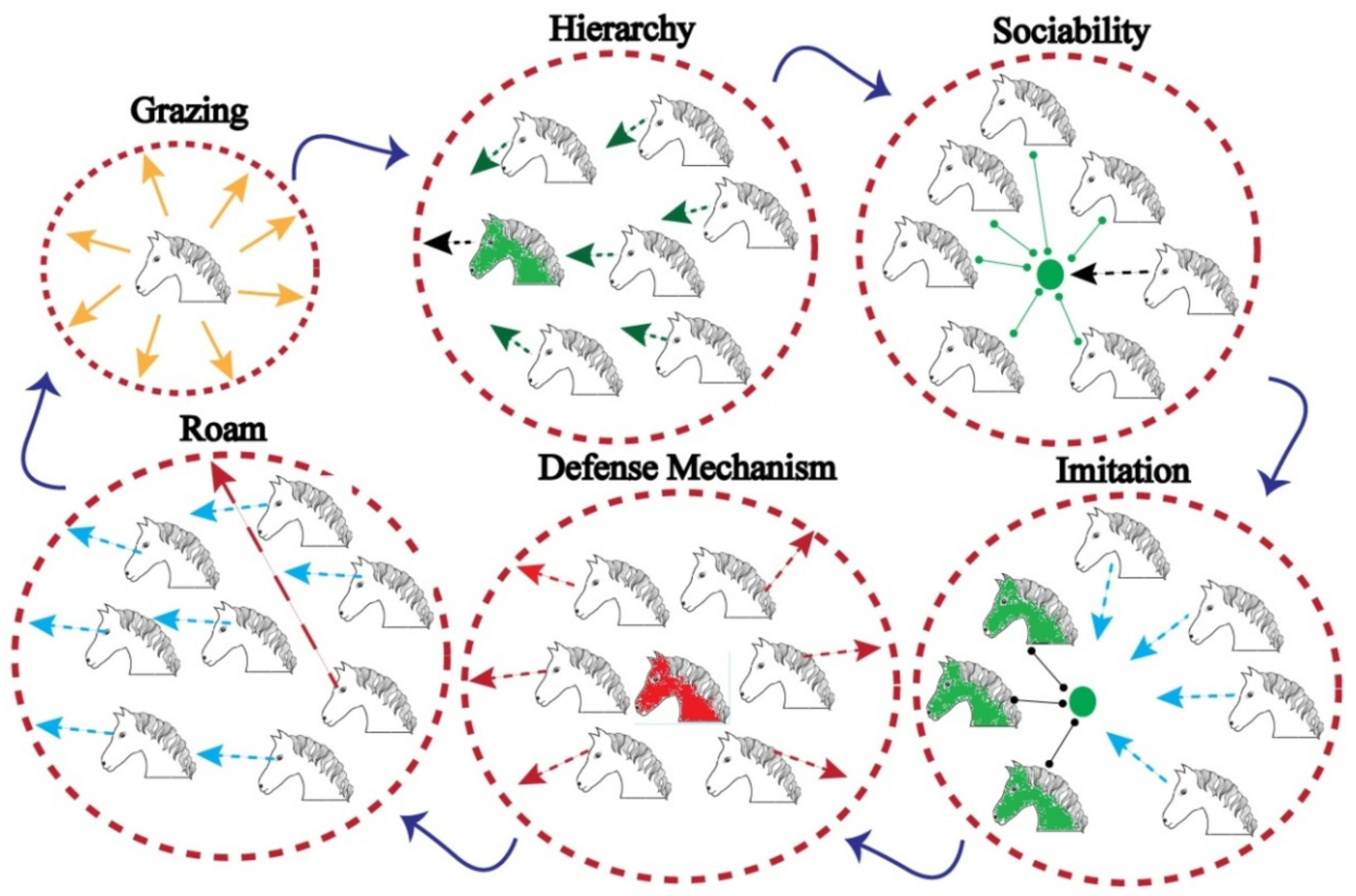
At various times in their lives, horses demonstrate different behaviors. A horse’s total lifespan is around 25–30 years [16]. In this case, $\delta$ represents horses between the ages of 0 and 5, $\gamma$ represents horses between the ages of 5 and 10, $\beta$represents horses between the ages of 10 and 15, and $\alpha$ denotes horses older than 15 years. To determine the age of the horses, each iteration should have a thorough matrix of answers. In this case, the matrix could be ordered based on the best replies, with the first 10% of the horses from the top of such an ordered matrix being chosen as $\alpha$horses. The β group is made up of the next 20% of the population. The γ and δ groups are responsible for 30% and 40% of the remaining horses, correspondingly. To determine the velocity vector, the methods to imitate the six actions of the various groups of horses are quantitatively executed.

Taking into account the following behavior patterns [15,16,17], Equations (2)–(5) may be represented as the motion vectors of horses of various ages throughout each cycle of the method.

$$Ve{l}_m^{iter,\alpha }=Gr{a}_m^{iter,\alpha }+DefMe{c}_m^{iter,\alpha }$$

(2)

$$Ve{l}_m^{iter,\beta }=Gr{a}_m^{iter,\beta }+H_m^{iter,\beta }+So{c}_m^{iter,\beta }+DefMe{c}_m^{iter,\beta }$$

(3)

$$Ve{l}_m^{iter,\gamma }=Gr{a}_m^{iter,\gamma }+H_m^{iter,\gamma }+So{c}_m^{iter,\gamma }+Im{t}_m^{iter,\gamma }+R{o}_m^{iter,\gamma }+DefMe{c}_m^{iter,\gamma }$$

(4)

$$Ve{l}_m^{iter,\delta }=Gr{a}_m^{iter,\delta }+I{m}_m^{iter,\delta }+R{o}_m^{iter,\delta }$$

(5)

These are the major phases in individual and social intelligence for horses.

3.1. Grazing (Gra)

Horses are roaming animals that eat grasses, plants, and other forage. They graze in pastures for between 16 and 20 h per day, with only a few hours of rest. Continuous eating is the term for this type of gradual grazing—you may have seen mares grazing in pastures when carrying their foals [17].

The grazing area for each horse is modeled using the HOA technique. As a result of the coefficient g, each horse grazes in certain locations, as shown in Figure 9. Horses graze at any age and for the rest of their lives. Grazing is implemented mathematically, in line with Equations (6) and (7).

$$Gr{a}_m^{iter,age}=g_{iter}\left(low+r\ast upp\right)(P_m^{\left(iter-1\right)}), age=\alpha , \beta , \gamma , \delta$$

(6)

$$g_m^{iter,age}=w_g\times g_m^{\left(iter-1\right),age},$$

(7)

Here, $Gr{a}_m^{iter, age}$ denotes the parameter of motion of the $i\mathrm{th}$ horse and illustrates the related horse’s ability to graze. The grazing variable lowers linearly at $w_g$ for each iteration. The variable “r” is an arbitrary value of between 0 and 1, while “low” and “upp” are the lower and upper boundaries of the grazing space, respectively. For all age groups, it is advised that “low” and “upp” should be set to 0.95 and 1.05, respectively. The coefficient g value is set to 1.5 in all range ages.

3.2. Hierarchy (H)

Horses are not self-sufficient [18]. They live their lives following a leader, and this is something that humans will do frequently. According to the rule of dominance [18], a mature stallion or a filly is likewise responsible for management in groups of wild horses.

The inclination of a group of horses to follow the lead of the most trained and powerful horse is regarded as the coefficient $h_m$ in HOA and is shown in Figure 9. So, at the middle ages of $\beta$ and $\gamma$ (aged 5–15 years), studies have demonstrated that horses follow the law of hierarchy [17]. Equations (8) and (9) can be used to define this (Section 3.6).

$$H_m^{iter,age}=h_m^{iter,age}(P_{lbh}^{\left(iter-1\right)}-P_m^{\left(iter-1\right)})$$

(8)

$$h_m^{iter,age}=h_m^{\left(-1+iter\right),age}\times w_h$$

(9)

Here, $H_m^{iter,age}$ illustrates the location of the best horse with the variable of velocity. The value $P_{lbh}^{\left(iter-1\right)}$ indicates the position of the best horse.

3.3. Sociability (Soc)

Horses need social interaction and may coexist with other animal species. Because wild horses may be hunted by predators, life in a group ensures their safety. Pluralism improves their survival odds and makes it easier to flee. Horses frequently fight each other owing to their social characteristics, and their very uniqueness is a cause of their anger. Some horses appear to enjoy being with other animals such as cattle and sheep, but they dislike being alone [17].

This behavior is depicted by element s as a movement toward the average location of other horses, as seen in Figure 9. Horses between the ages of 5 and 15 years are primarily interested in being with the herd, as shown by the given formulas:

$$So{c}_m^{iter,age}=so{c}_m^{iter,age}\left[\left(\frac{1}{N}{{\displaystyle \sum }}_{j=1}^N{P}_j^{\left(-1+iter\right)}\right)-P_m^{\left(-1+iter\right)}\right] age=\beta ,\gamma$$

(10)

$$so{c}_m^{iter,age}=so{c}_m^{\left(-1+iter\right),age}\times {\omega }_{soc}$$

(11)

In the above equations:

• $So{c}_m^{iter,age}$ describes the vector of social motion that is presented by the $i\mathrm{th}$ horse.
• $so{c}_m^{iter,age}$ shows the orientation of that horse in the direction of group $i\mathrm{th}$.
• iter, the iteration is reduced in every cycle, has a parameter of ${\omega }_s$.
• $N$ expresses the total number of horses.
• age represents the age range of each horse.

From an evaluation of these factors, the s coefficient for $\gamma$ and $\beta$ horses is derived.

Figure 9. Diagram representing grazing, hierarchy, sociability, imitation, defense mechanisms, and roam of the HOA.

Figure 9. Diagram representing grazing, hierarchy, sociability, imitation, defense mechanisms, and roam of the HOA.

3.4. Imitation (Im)

Horses copy one another and pick up on each other’s positive and negative habits, such as locating the best grazing spot [17]. In the current method, the imitation behavior of horses is also taken into account as the factor i. Young horses tend to imitate older ones, and this trait persists throughout their lives (see Figure 9, as explained in Equations (12) and (13)).

$$I{m}_m^{iter,age}=i{m}_m^{iter,age}\left[\left(\frac{1}{pN}{{\displaystyle \sum }}_{j=1}^{pN}{P}_j^{\left(-1+iter\right)}\right)-P^{\left(-1+iter\right)}\right] age=\gamma$$

(12)

$$i{m}_m^{iter,age}=i{m}_m^{\left(-1+iter\right),age}\times {\omega }_{im}$$

(13)

In the above equations:

• $I{m}_m^{iter,age}$ expresses the vector of motion that represents the $i\mathrm{th}$ horse around the average of the best horse at P position.
• $i{m}_m^{iter,age}$ shows the orientation of that horse in the direction of the group on the $i\mathrm{th}$ iteration. This is reduced in every cycle, with a parameter of ${\omega }_{im}$.
• $pN$ represents the number of horses in the best positions, where $p$ is 10% of the selected horses.
• ${\omega }_{im}$ is a reduction factor per cycle for $i_{iter}$.

3.5. Defense Mechanism (DefMec)

The attitude of horses reflects the fact that they have historically been preyed upon [17]. They use the fight-or-flight reaction to defend themselves. Their initial impulse is to flee. In addition, when trapped, they will buck. Horses battle for food and water to keep rivals at bay and to avoid dangerous locations where adversaries such as wolves may lurk [15,16,17,18].

In the HOA method, the horses’ defense mechanism works by fleeing away from those horses who exhibit improper or suboptimal behaviors, as illustrated in Figure 9. This factor characterizes their primary defense mechanism. As previously stated, horses must either run from or battle their foes. When possible, such a defensive system exists throughout the lifecycle of a young or adult horse. A negative coefficient in Equations (14) and (15) represents the horse’s defensive system, which keeps the animal away from dangerous situations.

$$\begin{gathered} DefMe{c}_m^{iter,age}=defme{c}_m^{iter,age}\left[\left(\frac{1}{qN}{{\displaystyle \sum }}_{j=1}^{qN}{P}_j^{\left(-1+iter\right)}\right)-P^{\left(-1+iter\right)}\right] age= \\ \alpha ,\beta ,\gamma \end{gathered}$$

(14)

$$defme{c}_m^{iter,age}=defme{c}_m^{\left(-1+iter\right),age}\times {\omega }_{defmec}$$

(15)

In the above equations:

• $DefMe{c}_m^{iter,age}$ describes the escape vector of the$i\mathrm{th}$ horse, based around the average position of a horse in the worst P position.
• $qN$ shows the number of horses in the worst positions, where $q$ is 20% of the total horses.
• ${\omega }_{defmec}$ represents the reduction factor per cycle for iIter that was calculated earlier.

3.6. Roam (Ro)

In the pursuit of food, horses move and graze across the countryside, moving from pasture to pasture [17]. The majority of horses are maintained in stables, although they preserve the aforementioned trait. A horse may abruptly change its grazing site. Horses are incredibly curious, and they frequently visit different pastures and get to know their surroundings. The horses may see each other through the side walls of their enclosures, and their desire for sociability is satisfied in an adequate stable [17,18].

The factor r is used to imitate this behavior in the algorithm, as nothing more than a random movement. Roaming is virtually never seen in horses while they are young, and it progressively fades as they mature. This process is depicted in Figure 9. Equations (16) and (17) show the roam variables. The flowchart of the HOA algorithm is given in Figure 10.

Figure 10. Flowchart of the HOA algorithm.

Figure 10. Flowchart of the HOA algorithm.

$$R{o}_m^{iter,age}=r{o}_m^{iter,age}\partial P^{\left(-1+iter\right)} age=\gamma ,\delta$$

(16)

$$r{o}_m^{iter,age}=r{o}_m^{\left(-1+iter\right),age}\times {\omega }_{ro}$$

(17)

Here, ${Ro}_m^{iter,age}$: is the arbitrary velocity vector of the $i\mathrm{th}$horse for just a local area search and an escape from local minima.

${\omega }_{ro}$ represents a reduction factor of ${ro}_m^{iter,age}$ per cycle.

By putting the results from Equations (6)–(17) into Equations (2)–(5), we can establish the generic velocity vector.

Velocity of δ horses at the age of 0–5 years:

$$\begin{gathered} Ve{l}_m^{iter,\delta }=\left[w_g\times g_m^{\left(iter-1\right),\delta }\left(low+r\ast upp\right)[P_m^{\left(iter-1\right)}]\right] \\ +i{m}_m^{\left(-1+iter\right),\delta }\times {\omega }_{im}\times \left[\left(\frac{1}{pN}{\displaystyle \sum }_{j=1}^{pN}{P}_j^{\left(-1+iter\right)}\right)-P^{\left(-1+iter\right)}\right] \\ +{ ro}_m^{\left(-1+iter\right),\delta }\times {\omega }_{ro}\times \partial P^{\left(-1+iter\right)} \end{gathered}$$

(18)

Velocity of γ horses at the age of 5–10 years:

$$\begin{gathered} Ve{l}_m^{iter,\gamma }=\left[w_g\times g_m^{\left(iter-1\right),\gamma }\left(low+r\ast upp\right)[P_m^{\left(iter-1\right)}]\right] \\ +h_m^{\left(-1+iter\right),\gamma }\times w_h\times [P_{lbh}^{\left(iter-1\right)}-P_m^{\left(iter-1\right)}] \\ +so{c}_m^{\left(-1+iter\right),\gamma }\times {\omega }_{soc}\times \left[\left(\frac{1}{N}{\displaystyle \sum }_{j=1}^N{P}_j^{\left(-1+iter\right)}\right)-P_m^{\left(-1+iter\right)}\right] \\ +i{m}_m^{\left(-1+iter\right),\gamma }\times {\omega }_{im}\times \left[\left(\frac{1}{pN}{\displaystyle \sum }_{j=1}^{pN}{P}_j^{\left(-1+iter\right)}\right)-P^{\left(-1+iter\right)}\right] \\ +{ro}_m^{\left(-1+iter\right),age}\times {\omega }_{ro}\times \partial P^{\left(-1+iter\right)} \end{gathered}$$

(19)

Velocity of β horses at the age of 10–15 years:

$$\begin{array}{c}Ve{l}_m^{iter,\gamma }=\left[w_g\times g_m^{\left(iter-1\right),\beta }\left(low+r\ast upp\right)[P_m^{\left(iter-1\right)}]\right]\\ +h_m^{\left(-1+iter\right),\beta }\times w_h\times [P_{lbh}^{\left(iter-1\right)}-P_m^{\left(iter-1\right)}]\\ +so{c}_m^{\left(-1+iter\right),\beta }\times {\omega }_{soc}\times \left[\left(\frac{1}{N}{\displaystyle \sum }_{j=1}^N{P}_j^{\left(-1+iter\right)}\right)-P_m^{\left(-1+iter\right)}\right]\\ -defme{c}_m^{\left(-1+iter\right),\beta }\times {\omega }_{defmec}\\ \times \left[\left(\frac{1}{qN}{{\displaystyle \sum }}_{j=1}^{qN}{P}_j^{\left(-1+iter\right)}\right)-P^{\left(-1+iter\right)}\right]\end{array}$$

(20)

Velocity of α horses at the age of 10–15 years:

$$\begin{array}{l}Ve{l}_m^{iter,\alpha }= \left[w_g\times g_m^{\left(iter-1\right),\alpha }\left(low+r\ast upp\right)[P_m^{\left(iter-1\right)}]\right]\\ -defme{c}_m^{\left(-1+iter\right),\alpha }\times {\omega }_{defmec}\\ \times \left[\left(\frac{1}{qN}{{\displaystyle \sum }}_{j=1}^{qN}{P}_j^{\left(-1+iter\right)}\right)-P^{\left(-1+iter\right)}\right]\end{array}$$

(21)

Some observations on how the HOA algorithm might be advantageous are as follows:

• The α horses will get the best reactions and also serve as role models for the rest. They take over the coaching role as they begin their hunt for the optimum reaction and develop an exploited strategy. When the characteristics of grazing and defensive mechanisms must be used, this behavior occurs.
• The β horses diligently look for the most likely ideal locations, paying great attention to α.
• The γ horses are created using all their inherent behaviors. They seem to be useful for both the explorative and exploitative phases, even though they exhibit both strong and arbitrary movements.
• Young horses seem to be more rambunctious and livelier, making them more suited to the exploring period.

The following are the main characteristics of our HOA method:

• The horse herd optimization algorithm (HOA) is a novel MPPT approach that has been developed.
• To collect the GM, the proposed approach needed fewer iterations.
• In PS and CPS situations, the proposed approach shows almost no oscillation and can collect GM.
• Experiments and findings show that the proposed approach with interims of rapid searching and minimal oscillation is preferable.
• A statistical study is performed to determine the algorithm’s efficiency, detecting speed, and steady-state reaction.

The HOA technique’s pseudo-code is shown in the box below.

(a)

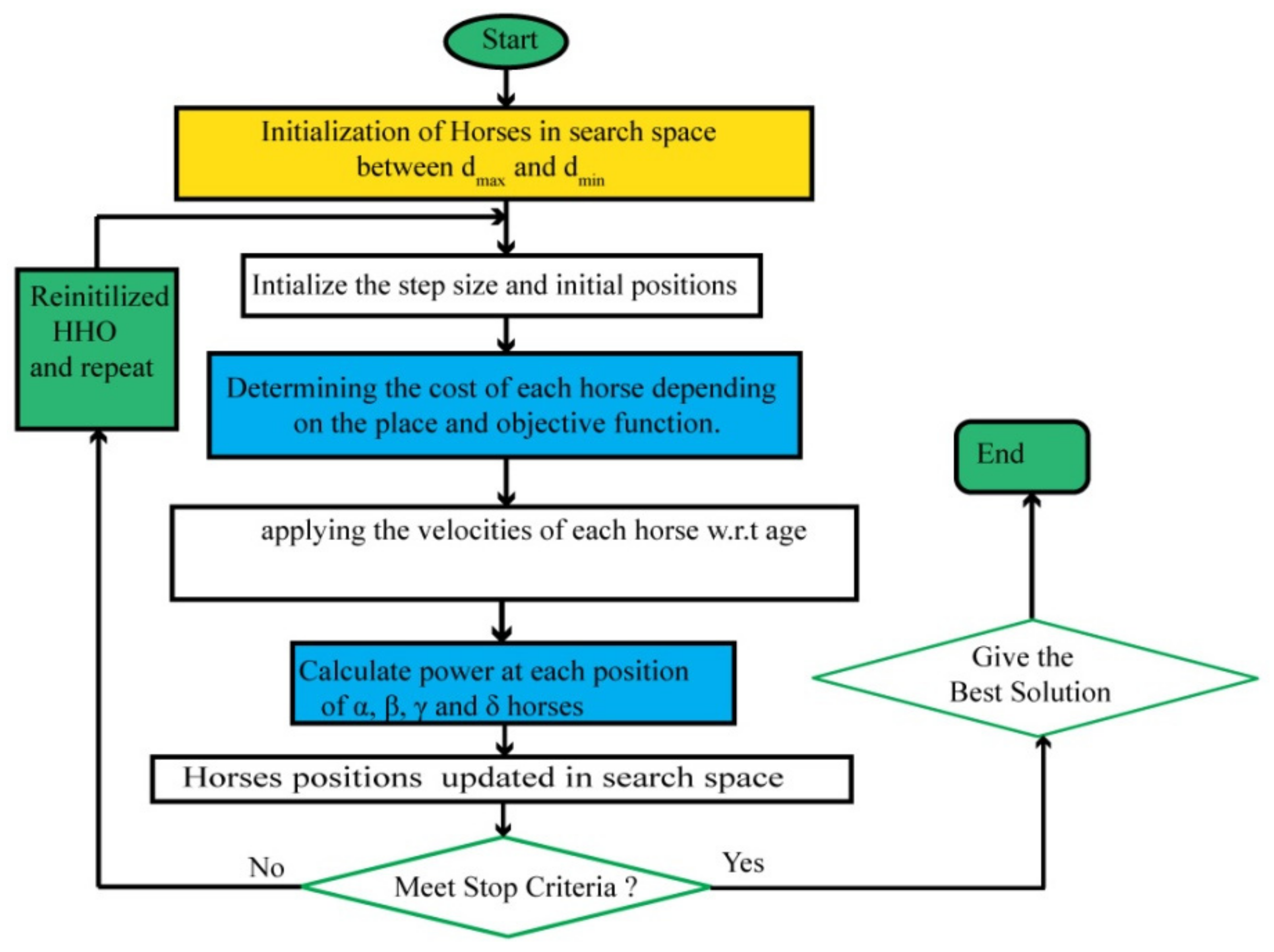
Basic configuration: providing variables with a boundary limit and other factors.

(b)

Initializing: creating a suitable space with a uniform random selection of horses.

(c)

Checking fitness level: determining the cost of each horse, depending on the place and objective function.

(d)

Evaluating age: assessing the ages of (α, β, γ, and δ) horses.

(e)

Implement the velocity: with respect to every horse’s age, apply the velocity.

(f)

Revise the position: updating the position of all horses in the search space.

(g)

End: if the stop criteria are not met, go to step (c).

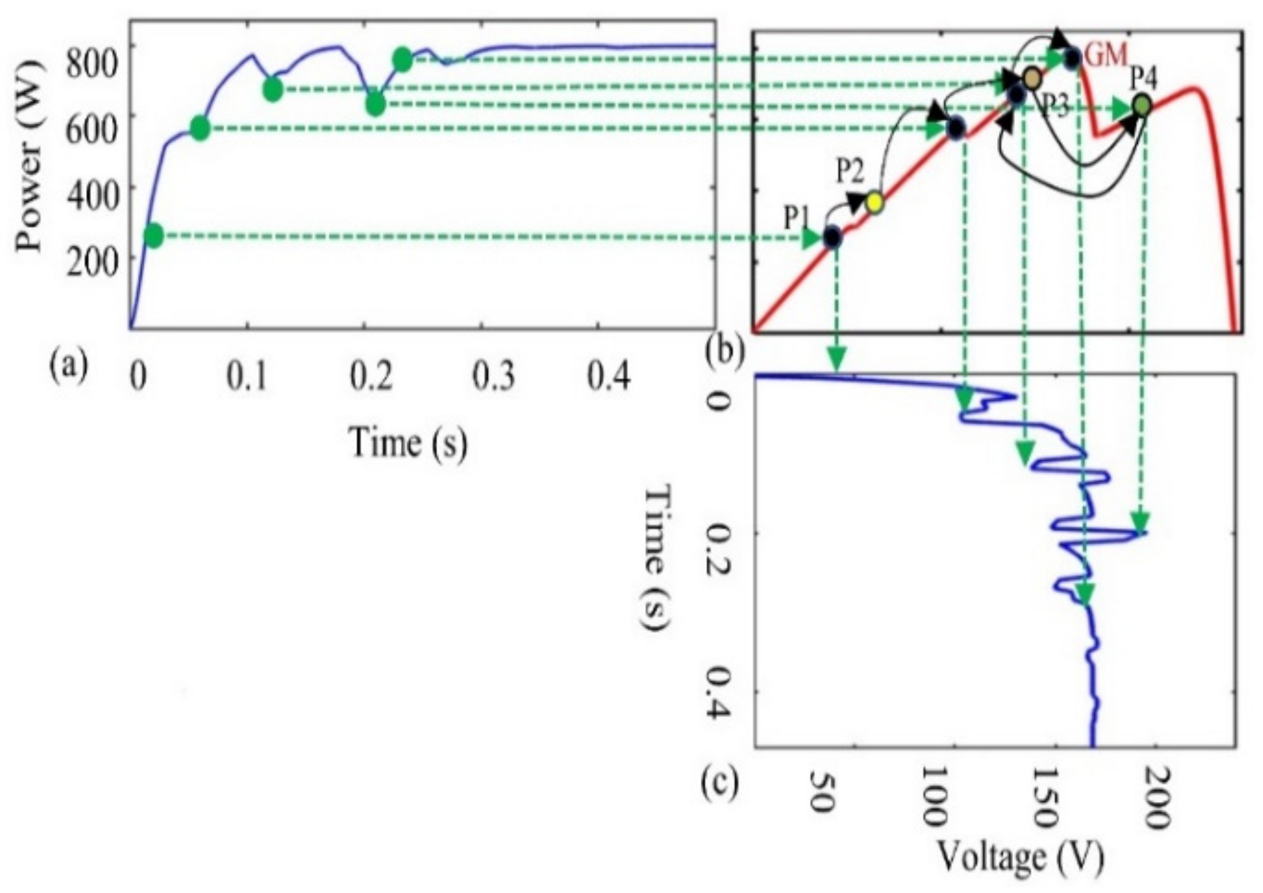
4. Tracking Mechanism of HOA

The tracking mechanism is illustrated in the flow chart of HOA in Figure 10. By using the transient value of the voltage at the output and the duty cycle (dc), the tracking behavior of HOA is presented. The partially shaded power-voltage curve is illustrated at the top right corner, shown in Figure 11b, in which there exists only one point; this point is GM, while the remaining three points are LM. In Figure 11b, HOA is initialized with four horses, named $P1$, $P2$,$P3,$ and $P4$. The efficiency of the PV system is affected by increasing or decreasing the number of horses; therefore, four horses are used here to achieve good performance from the HOA. The fitness is calculated for each horse by using the magnitude of power. The corresponding power of each horse at a distinct location determines the movement of a horse, and the expression (4) in Section 3 is used to update the movement of each horse. As illustrated in Figure 11b, point $P2$ has the highest fitness value; therefore, the output is given to $P2$. In the initial 45–55 milliseconds, the sudden increase in power is due to its highly efficient explorative/searching performance, controlled by $\left(10\right)$ and $\left(11\right)$. At the start, the exploration phase remains dominant until the 201-millisecond point. Therefore, it is difficult to track the GM. In Figure 11b, at 50 milliseconds, P2 encounters LM2. The remaining horses demonstrate lower fitness, and the controlled output remains unchanged for a few milliseconds in terms of the dc of the selected converter. However, other horses start searching for the best solution. When the horse is wedged in at LM, this indicates the minima of its personal best; in addition to this, it keeps searching, until and unless the horses explore an improved solution. It can be noticed that $P3$ is the best solution and the horses have left the $P2$ point, as shown in Figure 11b. The convergence of horses begins in the next 80 to 125 milliseconds. In the meantime, $P4$ starts searching for the new, fittest solution, resulting in a little surge at around 125 milliseconds. Now, $P3$ overtakes$P4$. Once more, LM3 is encountered, and the output of HOA becomes stagnant at LM3. In the meantime, the mechanism breaks the LM3 trap. The GM is obtained within 141 milliseconds, and it can be observed that all the horses settle at the GM successfully and the HOA reaches a state of equilibrium. During the searching process, large fluctuations of voltage transients are observed as an initial phase effect; finally, the oscillations produced by the voltage are considerably reduced and the HOA successfully tracks the GM. The power and voltage are tracked by HOA, present in Figure 11a,c, respectively.

HOA under Complex Partial Shading (CPS) Conditions

Most optimization algorithms for MPPT are unable to track the GM under CPS conditions. As mentioned earlier, HOA is proposed here specifically for this purpose. Therefore, we will proceed to discuss the CPS conditions in detail and the consequent impact of the HOA’s application. CPS occurs when myriad modules of PV cells, connected in series, are subjected to PS55. This extreme situation results in the formation of multiple close peaks of LM. Such a collection of local maxima is known as a cluster. Every cluster has its own maxima, named the cluster head maxima (CHM) [19,20].

A specific CPS case is shown in Figure 6, hereafter referred to as case 4. which will be later utilized to acquire the GM, using HOA, for the research work presented in this paper. The left half of the curve of P-V presents a cluster, including 4 MPPs. The corresponding power of LM, starting from left to right, is observed as 729.6 W, 898.3 W, 989.8 W, and 1080 W, respectively. The computed maximum power value of the cluster is 1080 W. Three MPPs exist in a cluster on the right half-curve. Their respective powers are observed as 1080 W, 1025 W, and 831 W, respectively, from right to left. At the extreme left peak, the maxima of the cluster head occur, which gives the global MPP.

It is clear that the cluster values of CHM1 and LM2 are quite close to each other, $1010 \mathrm{W}$ and $1025 \mathrm{W}$, having a minor difference of 14.5 W that comprises less than 2% of the maximum power. Consequently, this algorithm does not re-initialize the next epoch to track the MPP, due to being wedged in, and the horses may not find the area between CHM2 and GM. Additionally, in previous iterations, the vectors of velocity intentionally slow down the motion of the horses. For improved convergence and minimum oscillations, the slower motion in the previous iteration cycle is convenient. Undetected GM causes a remarkable $5.7\%$ loss of attainable power, due to a complicated PS. For GMPP tracking, which is present in the middle areas of the power and voltage characteristics curves, the HOA method is useful.

To resolve the abovementioned problem, a common search with a huge number of horses is used; however, by increasing the number of horses, there is an exponential increase in the resources needed for completing the communal interactivity. This causes an increase in cost, as well as computational complexity, while reducing the application range. Generally, when applying MPPT, 4 to 6 particles are used, and empirical outcomes are achievable by this efficient process [17]. Effective solutions are obtained in HOA by creating efficient groups, maintaining the space among adjacent horses, as well as initializing the process again. The procedure can be made even more efficient by initializing and moving the HOA particles, such that the scanned areas are skipped effectively. The highest exploration can be ensured via the horses’ mobility utilizing HOA.

5. Experimental Results

This section discusses four different scenarios, in which three cases represent four conditions of operation and one case represents twelve conditions of operation. For formulating the problem comprehensively, the different scenarios are chosen for comparing the results of HOA with those found using PSO, ACS, P&O, and DFO techniques. Case 1 presents the fast-changing nature of irradiance, Cases 2 and 3 pertain to the PS conditions, while Case 4 deals with the CPS condition. The final conclusions are drawn, based on the attained performance.

Table 1. Techniques for comparing the power, tracking, and efficiency with that of the HOA.

Method	Irradiance Scheme	Convergence Time (s)	GM Settle Time (s)	GM Existed	Power at GM	Power Tracking (W)	Energy Value (kWh)	Efficiency (%)
DFO	Case 1	0.24	0.28	Yes	1260	1259	1.66	99.9
	Case 2 PS	0.26	0.43	Yes	450	448.7	0.85	99.5
	Case 3PS	0.19	0.21	Yes	796	793.5	1.55	99.7
	Case 4CPS	0.19	0.22	Yes	1078	1075	2.12	99.8
HOA	Case 1	0.16	0.20	Yes	1260	1259.9	1.66	99.9
	Case 2 PS	0.19	0.37	Yes	450	449.7	0.86	99.8
	Case 3PS	0.19	0.22	Yes	796	795.8	2.12	99.9
	Case 4CPS	0.17	0.25	Yes	1078	1077	1.65	99.8
P&O	Case 1	0.12	0.12	Yes	1260	1237	0.46	98.1
	Case 2 PS	LM	LM	No	450	220	0.47	67.7
	Case 3PS	LM	LM	No	796	238	0.51	32.0
	Case 4CPS	LM	LM	No	1078	262	1.64	24.7
PSO	Case 1	0.47	0.70	Yes	1260	1257	0.83	94.6
	Case 2 PS	0.41	0.81	Yes	450	439.2	1.48	97.6
	Case 3PS	0.68	0.70	Yes	796	791.5	2.10	99.4
	Case 4CPS	0.42	0.50	Yes	1078	1068	1.65	99.2
ACS	Case 1	0.46	0.69	Yes	1260	1258	0.83	99.8
	Case 2 PS	0.30	0.84	Yes	450	420	1.49	95.5
	Case 3PS	0.35	0.45	Yes	796	778.6	2.10	97.8
	Case 4CPS	0.40	0.56	Yes	1078	1067	3.10	99.2

presents a detailed analysis of the results.

The performance analysis depends on different factors, including the time required for tracking, the convergence of power, the settling time, oscillations while in steady-state, transience in the voltage, currents, efficiency, and obtained power, as well as the energy used by the techniques to obtain the power. The results verify the conjecture that the HOA performs more efficiently compared to other optimization techniques.

Table 2. Case 1 to Case 3: levels of irradiance.

Cases	$\mathbf{Irradiance} {\mathbf{S}}_{\mathbf{i}}\left(\frac{\mathbf{k}\mathbf{W}}{{\mathbf{m}}^2}\right)$				${\mathbf{P}}_{\mathbf{max} }$
${\mathrm{C}}_{1-4}$	PV1	PV2	PV3	PV4	(W)
Case1Fast Changing	1, 0.7, 0.3	1, 0.7, 0.3	1, 0.7, 0.3	1, 0.7, 0.3	1260, 880, 380
Case2 (Partial Shading)	0.8	0.25	0.7	0.4	449.7
Case3 (Partial Shading)	0.5	0.8	1.0	0.9	796.1

shows the UIC and PS conditions, and the corresponding irradiance level received by the PV panels.

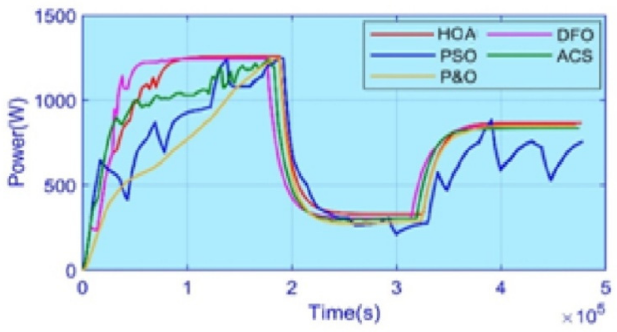
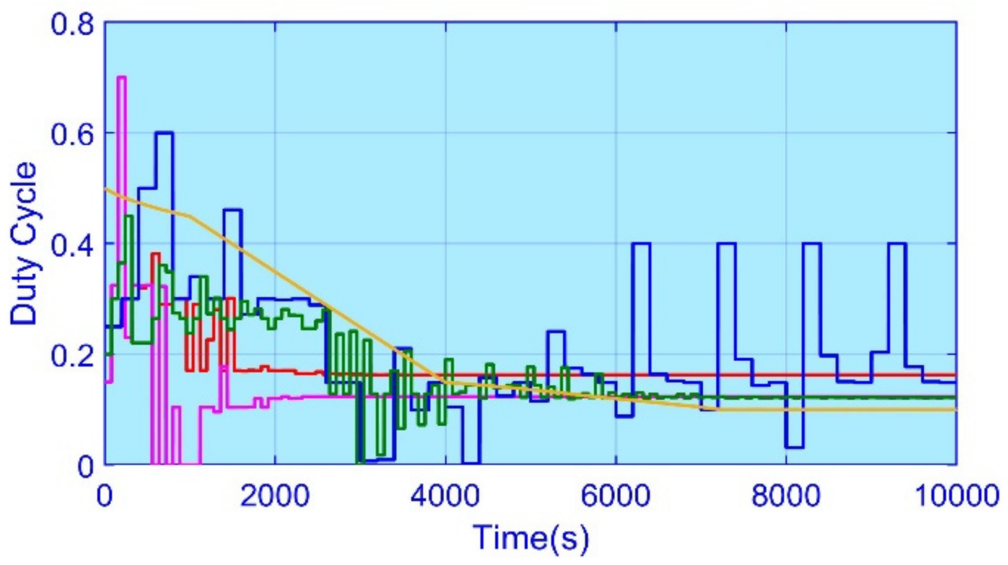
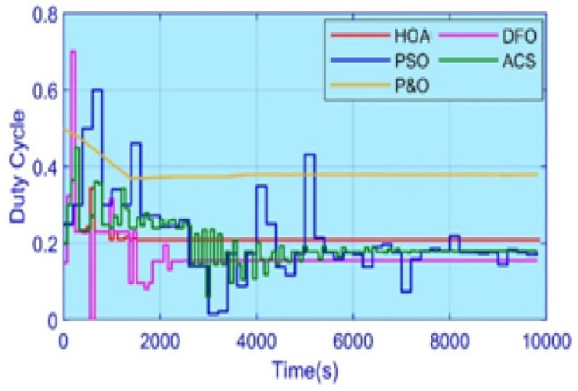
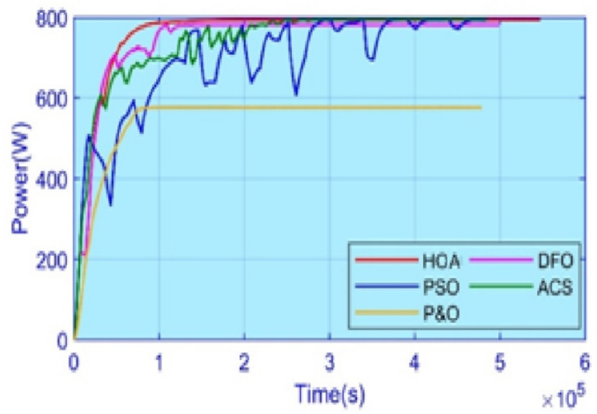
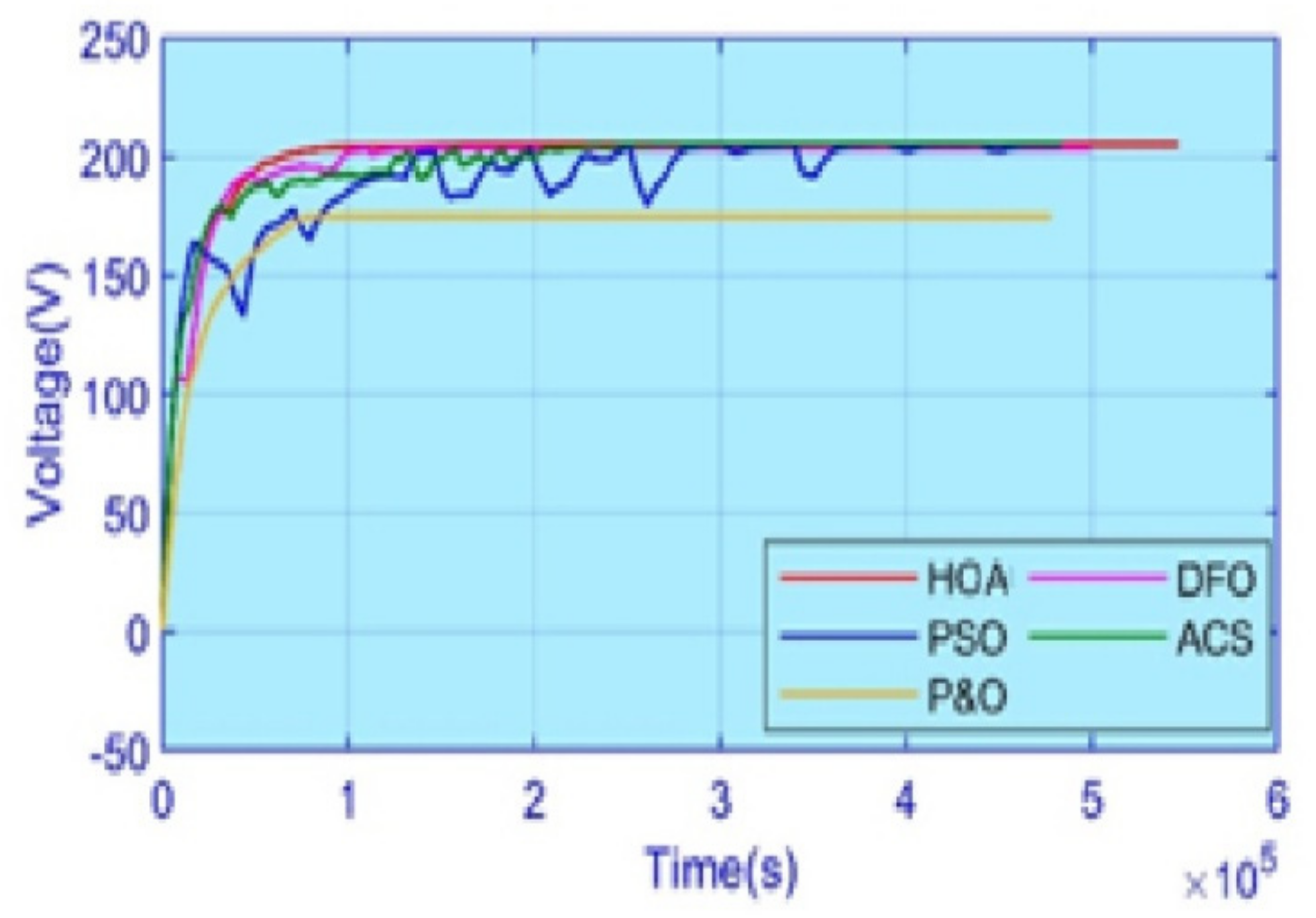
5.1. Case 1: Fast-Changing Irradiance

All the modules of the PV cells are provided in Case 1 with equal irradiances, but the level of irradiance changes with respect to time, which is called fast-changing irradiance. Table 2 shows the irradiances’ pattern. The MPP is shifted by the change in irradiance, as shown in Figure 4. The power comparison of HOA with the existing techniques is shown in Figure 12. HOA achieves a maximum value of efficiency in terms of power in the initial interval, when it reaches 1260 W. For comparison with the power efficiencies achieved by HOA, note that DFO, PSO, ACS, and P&O are 1259.5 W, 1257 W, 1239 W, and 1210 W, respectively. These values show that HOA achieved 99.98% efficiency. Case 1 exhibits 3 different regions, based on the values of irradiance. Considering the mean value is more suitable for measuring the efficiency of the competing techniques, since the value of irradiance changes with reference to time [2]. The mean values of the powers attained by HOA, DFO, PSO, ACS, and P&O are 834.2 W, 822.9 W, 820.1 W, 828 W, and 819.4 W, respectively, indicating the greatest attained average value was achieved with the HOA. The HOA generates about 6–33 W more, compared with the other algorithms. The total achievable efficiency by HOA, DFO, PSO, ACS, and P&O, which is the ratio of average to the highest power value, is 99.27%, 97.96%, 97.91%, 97.95%, and 98.79%, respectively. The ranking of these techniques in terms of power is as follows: HOA > DFO > PSO > ACS > P&O. The measured time of tracking of HOA, DFO, PSO, ACS, and P&O is 0.14 s, 0.18 s, 0.45 s, 0.47 s, and 0.33 s, respectively. The value of the settling time is calculated as 0.25 s, 0.25 s, 0.38 s, 0.62 s, and 0.70 s for HOA, DFO, PSO, ACS, and P&O, respectively. The HOA tracking and settling time is 50% faster for attaining the GM. The overshoot response in HOA is faster and aids in the prevention of unwanted oscillations, which may result in power loss. There is a convergence of P&O with GM, although it does not stop at the GM because of the continuously produced oscillations due to perturbations. The value of oscillations produced by P&O is 21 W; in the initial 0–2 s interval, there is an oscillation between 1259 W and 1238 W.

The dc or the duty ratio is the parameter to be controlled, as shown in Figure 13. The HOA successfully reduces the oscillation value to less than or equal to 1 W, resulting in a 95.24% reduction in the value of oscillations. The arbitrary oscillations by ACS and PSO remain quite high. Figure 12 indicates that PSO demonstrated the highest oscillations. ACS also produced random fluctuations. The transience caused by the voltage is shown in Figure 14.

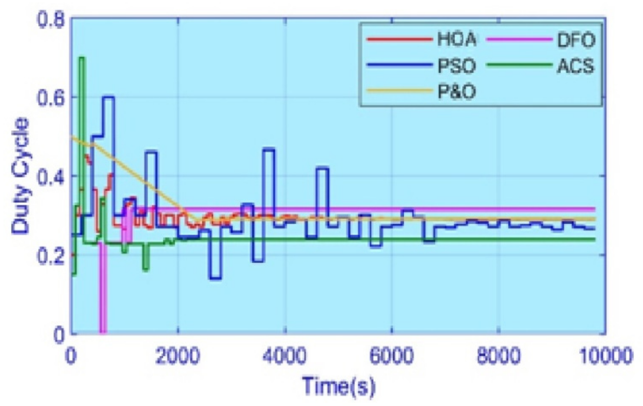
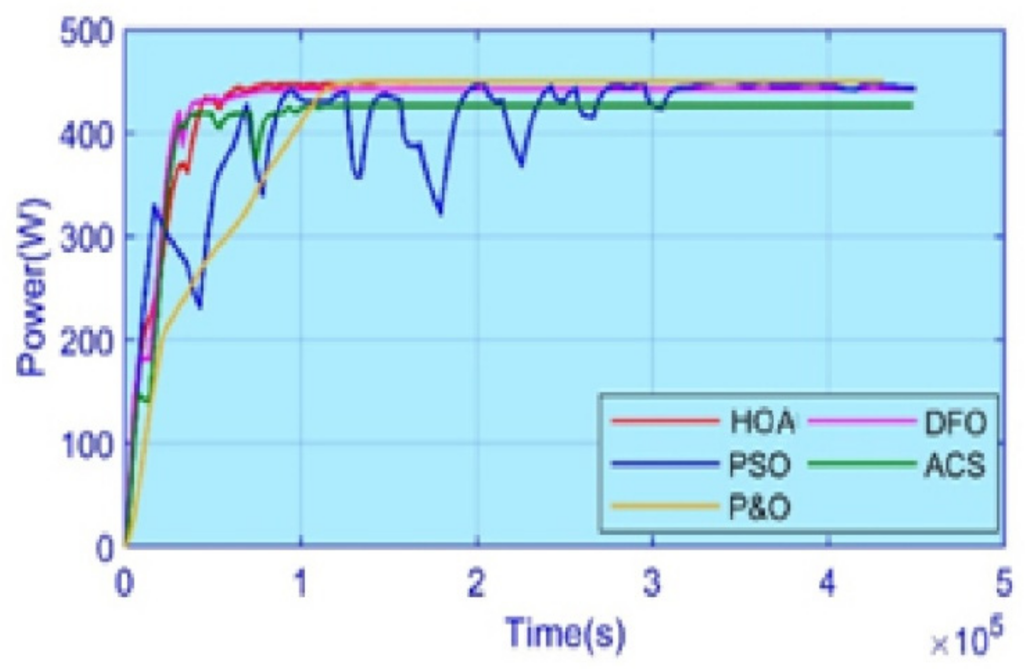
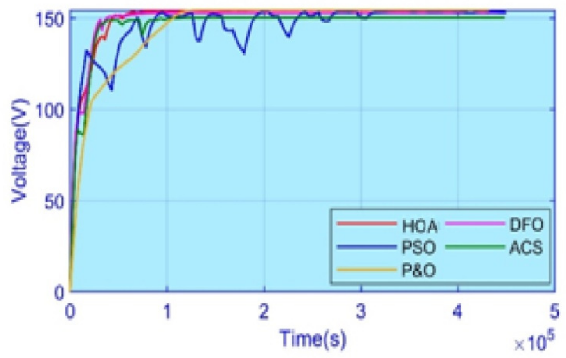
5.2. Case 2: PS Scenario 1

The value of global MPP lies at 450 W in Case 2. Figure 5 shows the curves of P-V and Table 2 gives the order in which the irradiance follows. The duty cycle comparison is presented in Figure 15. Some MPPT techniques utilize the method of making selections on a random basis to search the particles for breaking LM [15]. ACS and PSO algorithms show a high level of random behaviour. For generating unwanted variations, both methods employ arbitrary increases in the step size of the dc. The settling time of the ACS and PSO algorithms is large compared to that of the HOA. The HOA demonstrates almost zero oscillations in the equilibrium state at the global MPP. Figure 15 compares the power obtained by the HOA, DFO, PSO, ACS, and P&O algorithms. The calculations of the efficiency and the power are made against the global MPP, which is located at 450 W. The HOA demonstrates 99.94% efficiency, compared to 99.77% for DFO, 99.55% for PSO, 97.93% for ACS, and P&O, 99.90%; thus the HOA could reliably be called the most efficient technique for tracking the global MPP so far. The GM rapid-tracking and ordered settling time indicates the robustness of the MPPT method. Simulation results, based on the experiments, indicate that on average, the HOA, DFO, PSO, ACS, and P&O take 0.14 s, 0.19 s, 0.68 s, 0.30 s, and 0.22 s, respectively. Figure 16 and Figure 17 show the stable power and voltage produced by the HOA.

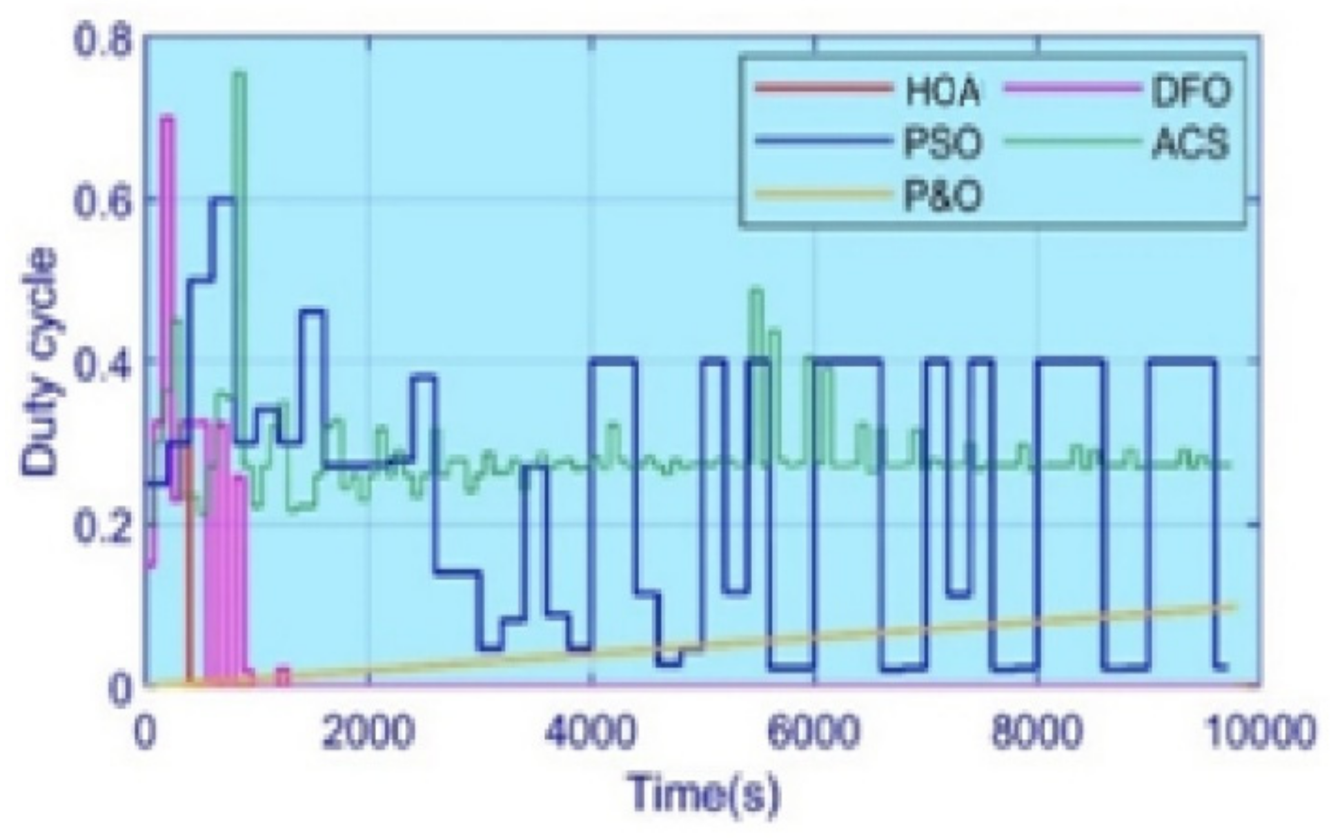
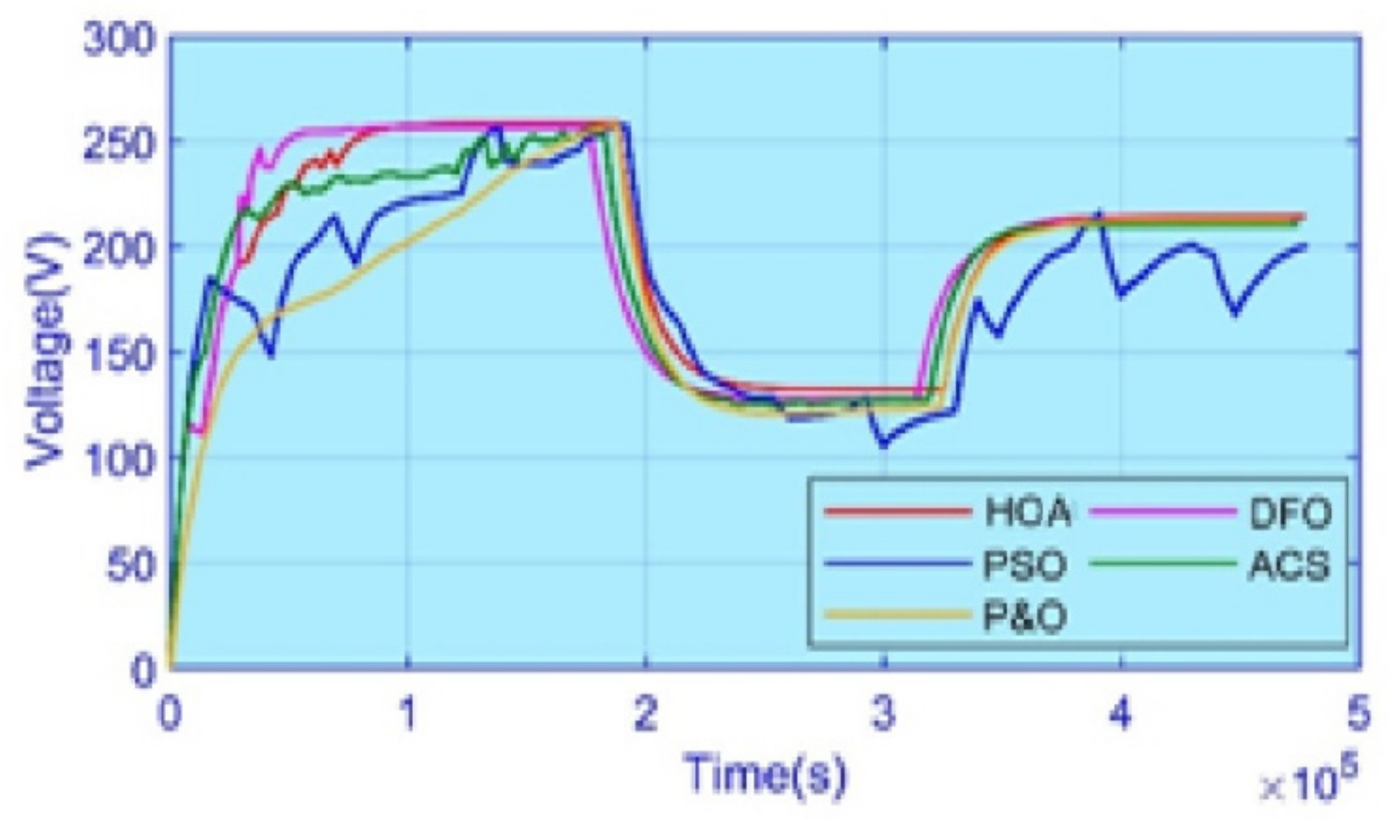
5.3. Case 3: PS Scenario 2

Table 2 shows the values of irradiance under the PS, while Figure 5 displays the equivalent curves of P-V, respectively. Three LMs and one GM are shown in the red curve, with a value of 796 W. P&O fails in tracking the GM by getting stranded in the area that is on the left of the P-V curves, thus limiting its efficiency value by the LM’s corresponding power.

Figure 18 shows the resultant power values, while Figure 19 demonstrates the control that the duty cycle provides. Figure 20 shows the voltage values. The peak value of power under the condition of PS, obtained by HOA, DFO, PSO, ACS, and P&O, is 795.1 W, 794.4 W, 785 W, 794.6 W, and 580 W, respectively. The maximum value of efficiency obtained is 99.88% and 99.80% by HOA and DFO, respectively; however, P&O obtains the minimum efficiency at around 49.40% and is stuck at LM1. The HOA, DFO, PSO, ACS, P&O have tracking times of 0.18 s, 0.18 s, 0.41 s, 0.39 s, and 0.45 s, respectively, while 0.40 s, 0.46 s, 0.56 s, 0.81 s, and 0.84 s are their times to settle, respectively. The HOA and DFO algorithm’s performances are almost equivalent while tracking the GM. The HOA tracks faster by 19%, thus settling in less than 455 ms for the GM. Due to rapid tracking, the unwanted oscillations are removed, while increasing the robustness. The P&O time for tracking is neglected here because it falls into the LM and is thus unable to locate the GM. This exceptional performance capability of HOA is shown in Case 3, which is followed by DFO, PSO, ACS, and P&O. Although the efficiency achieved by PSO is 97.61%, arbitrary oscillations can be seen in the values of voltage and current. ACS exhibits the same behavior, which in a normal operating situation is undesirable. Power converges 1–4% more in the case of the HOA algorithm, having less than a 1 W ripple, and, in the iteration cycles in the upcoming stages, the oscillations become zero. There are negligible oscillations in the curves of voltage as the output becomes stable under the HOA, as depicted in Figure 20. The duty cycle updates during every epoch, as shown in Figure 17, demonstrating the detection and convergence of HOA to GM with the fewest iterations and showing its superiority.

5.4. Case 4: Complex Partial Shading

This case discusses the CPS situation presented in Figure 6, where arrays of PV cells are serially joined together in the scenario mentioned in Table 3. Figure 21 compares the results of the power comparison. The DC-DC Cuk converter duty cycle measures the controlling activity depicted in Figure 21. The tracked power by the HOA, DFO, PSO, ACS, and P&O is 1079.3 W, 1079.1 W, 1060 W, 890 W, 510 W, respectively. The HOA achieved 99.93% efficiency, while the DFO was 99.92%, PSO 98.7, and ACS 94.7; P&O achieved the lowest power conversion efficiency of 67.4% among all the algorithms. Figure 22 shows that, as desired, the HOA can track the global MPP by utilizing the minimum iterations. Under the HOA and DFO models, there are minimal oscillations; the comparison between voltages is shown in Figure 23. The HOA exhibits the advantages of stable output and steady current.

Table 3. Irradiance level of CPS Cases.

Cases	$\mathbf{Irradiance} {\mathbf{S}}_{\mathbf{i}}\left(\frac{\mathbf{k}\mathbf{W}}{{\mathbf{m}}^2}\right)$				${\mathbf{P}}_{\mathbf{max} }\left(\mathbf{W}\right)$
Case4	PV1 = 0.4	PV2 = 0.2	PV3 = 0.6	PV4 = 0.3	1078
	PV5 = 0.5	PV6 = 0.4	PV7 = 0.2	PV8 = 0.3
	PV9 = 1.00	PV10 = 0.8	PV11 = 0.7	PV12 = 1.0

Table 3. Irradiance level of CPS Cases.

Cases	$\mathbf{Irradiance} {\mathbf{S}}_{\mathbf{i}}\left(\frac{\mathbf{k}\mathbf{W}}{{\mathbf{m}}^2}\right)$				${\mathbf{P}}_{\mathbf{max} }\left(\mathbf{W}\right)$
Case4	PV1 = 0.4	PV2 = 0.2	PV3 = 0.6	PV4 = 0.3	1078
	PV5 = 0.5	PV6 = 0.4	PV7 = 0.2	PV8 = 0.3
	PV9 = 1.00	PV10 = 0.8	PV11 = 0.7	PV12 = 1.0

Figure 21. Comparison of the HOA duty-cycle for Case 4.

Figure 21. Comparison of the HOA duty-cycle for Case 4.

Figure 22. Comparison of the HOA power for Case 4.

Figure 22. Comparison of the HOA power for Case 4.

For tracking or trailing the GM, the HOA, PSO, ACS, and DFO take 0.15 s, 0.42 s, 0.40 s, and 0.19 s, respectively, while the time to settle is 0.22 s, 0.31 s, 0.51 s, and 0.19 s, respectively. Comparing the results of the demonstration shows that the shortest settling time is from the HOA, followed by the DFO. The HOA settled at 0.22 s and under CPS conditions, and it was faster by 56 ms–300 ms on average, compared to the remaining methods. The performance rating of these techniques is HOA > DFO > ACS > PSO > P&O.

Figure 23. Comparison of the HOA voltage for Case 4.

Figure 23. Comparison of the HOA voltage for Case 4.

5.5. Efficiency and Performance Evaluation

On the basis of a statistical evaluation of HOA with competing algorithms, a performance evaluation has been carried out that helped to examine the common characteristics among the techniques. Conventionally, the P&O technique is rapid and easily implementable, as control depends on the gradient. Due to the oscillations, LM achieved and power wastage in the surroundings of MPP was created, thus making P&O an inconvenient choice for high-efficiency applications. PSO can locate GMPP with 99% efficiency under the conditions of PS, which was less in the case of CPS. ACS caused undesirable fluctuations while achieving an efficiency of 93–98%. The ACS took 820 ms to find the GM. The HOA successfully equipped the transient and steady-state oscillations. The overshoot offered by the HOA in response is the lowest compared to the other techniques and the efficiency value outperforms in every operating condition, up to 98%.

The novel HOA technique presented herein can track the global MPP in 95–310 ms in comparison to the time required by the other computing techniques. The HOA achieves 99.4% efficiency, on average, and performs very well among the rest of the competing techniques. Under the HOA, the oscillations decrease to less than 1 W, thus increasing the efficiency of re-tracking. Table 1 summarizes the results of all the respective techniques. According to Case 1, HOA outperforms during the transient phase, when it is exploring the optimum result, confirming it has the best ability to re-track. In Cases 2 to 3, other techniques are less efficient for converging power, while bio-inspired methods are more successful in locating the GM. Case 4 demonstrates the capability of the HOA to tackle the CPS scenario. There is a compromise in the PSO’s performance due to random initialization, as in other techniques, even after reaching the global MPP.

6. Conclusions

An MPPT method that is based on the HOA is presented in this paper with a Cuk converter. The assessment analysis of the HOA method has been performed qualitatively and quantitatively, versus the DFO, ACS, P&O, and PSO algorithms. Experimental results based on simulations are presented for four distinct scenarios that represent rapidly changing irradiance, in terms of the PS, along with CPS conditions. The outcomes confirm the effectiveness of the HOA method and show that it outperforms other optimization algorithms, in terms of the searching time of GM, the efficiency of power consumption, and oscillation reduction. Therefore, it is concluded that for increasing the performance of PV systems in different operating conditions related to PS and CPS, it is efficient to employ the MPPT method, which is based on an HOA with a Cuk converter.

References

1. Capuano, L. U.S. Energy Information Administration’s International Energy Outlook 2020; US Department of Energy: Washington, DC, USA, 2020; p. 7. Available online: https://www.Eia.Gov/Outlooks/Ieo/ (accessed on 20 September 2021).
2. Eldin, A.H.; Refaey, M.; Farghly, A. A Review on Photovoltaic Solar Energy Technology and its Efficiency. In Proceedings of the 17th International Middle-East Power System Conference (MEPCON’15), Mansoura, Egypt, 15–17 December 2015; pp. 1–9. [Google Scholar]
3. Sarwar, S.; Javed, M.Y.; Jaffery, M.H.; Arshad, J.; Rehman, A.U.; Shafiq, M.; Choi, J.-G. A Novel Hybrid MPPT Technique to Maximize Power Harvesting from PV System under Partial and Complex Partial Shading. Appl. Sci. 2022, 12, 587. [Google Scholar] [CrossRef]
4. Javed, M.Y.; Hasan, A.; Rizvi, S.T.H.; Hafeez, A.; Sarwar, S.; Telmoudi, A.J. Water Cycle Algorithm (WCA): A New Technique to Harvest Maximum Power from PV. Cybern. Syst. 2021, 1–23. [Google Scholar] [CrossRef]
5. Javed, M.Y.; Mirza, A.F.; Hasan, A.; Rizvi, S.T.H.; Ling, Q.; Gulzar, M.M.; Safder, M.U.; Mansoor, M. A Comprehensive Review on a PV Based System to Harvest Maximum Power. Electronics 2019, 8, 1480. [Google Scholar] [CrossRef] [Green Version]
6. Radjai, T.; Rahmani, L.; Mekhilef, S.; Gaubert, J.P. Implementation of a modified incremental conductance MPPT algorithm with direct control based on a fuzzy duty cycle change estimator using dSPACE. Sol. Energy 2014, 110, 325–337. [Google Scholar] [CrossRef]
7. Mohanty, P.; Bhuvaneswari, G.; Balasubramanian, R.; Dhaliwal, N.K. MATLAB based modeling to study the performance of different MPPT techniques used for solar PV system under various operating conditions. Renew. Sustain. Energy Rev. 2014, 38, 581–593. [Google Scholar] [CrossRef]
8. Krishna, K.S.; Kumar, K.S. A review on hybrid renewable energy systems. Renew. Sustain. Energy Rev. 2015, 52, 907–916. [Google Scholar] [CrossRef]
9. Zafar, M.H.; Khan, N.M.; Mirza, A.F.; Mansoor, M.; Akhtar, N.; Qadir, M.U.; Khan, N.A.; Moosavi, S.K.R. A novel meta-heuristic optimization algorithm based MPPT control technique for PV systems under complex partial shading condition. Sustain. Energy Technol. Assess. 2021, 47, 101367. [Google Scholar] [CrossRef]
10. Mohapatra, A.; Nayak, B.; Das, P.; Mohanty, K.B. A review on MPPT techniques of PV system under partial shading condition. Renew. Sustain. Energy Rev. 2017, 80, 854–867. [Google Scholar] [CrossRef]
11. Mirza, A.F.; Ling, Q.; Javed, M.Y.; Mansoor, M. Novel MPPT techniques for photovoltaic systems under uniform irradiance and Partial shading. Sol. Energy 2019, 184, 628–648. [Google Scholar] [CrossRef]
12. Mansoor, M.; Mirza, A.F.; Ling, Q. Harris Howk optomization-Based MPPT Control for PV Systems under Partial Shading Conditions. J. Clean. Prod. 2020, 274, 1–19. [Google Scholar] [CrossRef]
13. Farh, H.M.H.; Eltamaly, A.M. Maximum Power Extraction from the Photovoltaic System under Partial Shading Conditions. Smart Energy Grid Des. Isl. Ctries 2020, 107–129. [Google Scholar] [CrossRef]
14. Rezk, H.; Al-Oran, M.; Gomaa, M.R.; Tolba, M.A.; Fathy, A.; Abdelkareem, M.A.; Olabi, A.; El-Sayed, A.H.M. A novel statistical performance evaluation of most modern optimization-based global MPPT techniques for partially shaded PV system. Renew. Sustain. Energy Rev. 2019, 115, 109372. [Google Scholar] [CrossRef]
15. Mills, D.S.; McDonnell, S.M.; McDonnell, S. (Eds.) The Domestic Horse: The Origins, Development and Management of Its Behaviour; Cambridge University Press: Cambridge, UK, 2005. [Google Scholar]
16. Krueger, K.; Heinze, J. Horse sense: Social status of horses (Equus caballus) affects their likelihood of copying other horses’ behavior. Anim. Cogn. 2008, 11, 431–439. [Google Scholar] [CrossRef] [PubMed]
17. MiarNaeimi, F.; Azizyan, G.; Rashki, M. Horse herd optimization algorithm: A nature-inspired algorithm for high-dimensional optimization problems Knowledge-Based. Systems 2021, 213, 106711. [Google Scholar] [CrossRef]
18. Bogner, F. A Comprehensive Summary of The Scientific Literature on Horse Assisted Education in Germany. Ph.D. Thesis, Van Hall Larenstein, Leeuwarden, The Netherlands, 2011. [Google Scholar]
19. Mansoor, M.; Mirza, A.F.; Ling, Q.; Javed, M.Y. Novel Grass Hopper optimization based MPPT of PV systems for complex partial shading conditions. Sol. Energy 2020, 198, 499–518. [Google Scholar] [CrossRef]
20. Mirza, A.F.; Mansoor, M.; Ling, Q.; Yin, B.; Javed, M.Y. A Salp-Swarm Optimization based MPPT technique for harvesting maximum energy from PV systems under partial shading conditions. Energy Convers. Manag. 2020, 209, 112625. [Google Scholar] [CrossRef]
Figure 1. An optimized PV system diagram.
Energies 15 01880 g001
Figure 2. Circuit diagram of the Cuk converter.
Energies 15 01880 g002
Figure 3. Cases of uniform irradiance and partial shading.
Energies 15 01880 g003
Figure 4. The voltage–power curve under UIC.
Energies 15 01880 g004
Figure 5. The voltage–power curve under PSC.
Energies 15 01880 g005
Figure 6. Cluster formulation of the CPS scenario.
Energies 15 01880 g006
Figure 7. IV curves under PS conditions.
Energies 15 01880 g007
Figure 8. PV curves under PS conditions.
Energies 15 01880 g008
Figure 11. The tracking mechanism of the HOA through P-V curve (a) power-time curve, (b) GM tracking curve and (c) voltage-time curve.
Energies 15 01880 g011
Figure 12. Comparison of HOA power for Case 1.
Energies 15 01880 g012
Figure 13. Comparison of the HOA duty-cycle for Case 1.
Energies 15 01880 g013
Figure 14. Comparison of HOA voltage for Case 1.
Energies 15 01880 g014
Figure 15. Comparison of HOA duty cycles for Case 2.
Energies 15 01880 g015
Figure 16. Comparison of the HOA power for Case 2.
Energies 15 01880 g016
Figure 17. Comparison of HOA voltage for Case 2.
Energies 15 01880 g017
Figure 18. Comparison of the HOA duty-cycle for Case 3.
Energies 15 01880 g018
Figure 19. Comparison of the HOA power for Case 3.
Energies 15 01880 g019
Figure 20. Comparison of the HOA voltage for Case 3.
Energies 15 01880 g020