Local Path Planning for Autonomous Vehicles Based on the Natural Behavior of the Biological Action-Perception Motion

Abstract

Local path planning is a key task for the motion planners of autonomous vehicles since it commands the vehicle across its environment while avoiding any obstacles. To perform this task, the local path planner generates a trajectory and a velocity profile, which are then sent to the vehicle’s actuators. This paper proposes a new local path planner for autonomous vehicles based on the Attractor Dynamic Approach (ADA), which was inspired by the behavior of movement of living beings, along with an algorithm that takes into account four acceleration policies, the ST dynamic vehicle model, and several constraints regarding the comfort and security. The original functions that define the ADA were modified in order to adapt it to the non-holonomic vehicle’s constraints and to improve its response when an impact scenario is detected. The present approach is validated in a well-known simulator for autonomous vehicles under three representative cases of study where the vehicle was capable of generating local paths that ensure the security of the vehicle in such cases. The results show that the approach proposed in this paper is a promising tool for the local path planning of autonomous vehicles since it is able to generate trajectories that are both safe and efficient.

1. Introduction

Autonomous vehicles, both non-electrical and electrical, have the potential to change all mobility paradigms, improving safety, optimizing arrival, destination time, energy consumption, to name just a few improvements [1]. For those reasons, in the last decade, the different topics related to create fully autonomous vehicles were developed with impetus by several universities and automotive companies. The development of an autonomous vehicle can be divided into layers, mainly in three vast areas: state estimation and localization, visual perception, and motion planning [2]. All these areas have their challenges, with non-trivial tasks.

For instance, state estimation and localization generally are treated as two complementary sections. State estimation refers to the vehicle’s body dynamic state estimation and tire-road interaction estimation. Indeed, the vehicle dynamic state estimation, which can be further split into kinematics-based methods and dynamics-oriented approaches. In contrast localization is an approximation of the vehicle’s position for a given situation. Interested readers on those topics are referred to [3,4,5] and the references therein. On the other hand, visual perception covers aspects related with the driving surroundings, comprising the available driving areas and neighboring obstacles’ positions, speeds, and even prediction of their upcoming situations. The interested reader on those topics can review [6,7,8,9] and the references therein.

This manuscript is focused on motion planning (MP). The MP is the set of instructions that consider the state of the ego-vehicle (velocity, inclination, geo-reference, among others), the vehicle’s surrounding environment (e.g., dynamic, and static obstacles, drivable spaces), traffic rules, and allowed maneuvers, to generate a collision-free trajectory and a velocity profile that must be followed by the autonomous vehicle. The MP can be divided into four hierarchical tasks [10,11], each one assigned as follows: (I) mission planner or global path planning, (II) behavioral planner, (III) local path planning, and (IV) local feedback control.

Mission planner or global path planning refers to the step of achieving the most excellent path or at least an allowable estimation to it. Generally, the best path means to achieve an optimal one, in the sense that the resulting path arises from reaching one or more desired objective for instance, a path to achieve the least amount of time, the less dangerous maneuver, etc. On the other hand, behavioral planner can be understood as the device that perform knowledgeable choices depending on the real-time perception feedback and the calculated recommended path.

In contrast, local feedback control includes the overall actuator servos for the different autonomous vehicle subsystems (steering, brakes, engine, among others). The interested reader on those topics can review [12,13,14,15,16,17,18,19] and the references therein. This manuscript is focused on the MP’s local path planning.

This paper proposes a new way to plan the local path based on an approach that emulates the natural biological behavior of movement, called the Attractor Dynamic Approach (ADA) [20]. Originally, the ADA was proposed in the field of mobile robotics, and it was successfully implemented in such area. Due to its performance, it is an approach that may be scaled for the field of intelligent vehicles. However, there are some issues that must be overcome to successfully implemented it on autonomous vehicles. One of the more important drawbacks that the original ADA presents is certain instability when there are a high number of obstacles nearby; however, in a driving vehicle’s scenario, it is rare that there are only a few obstacles in the environment. Furthermore, its mathematical functions are set in a way that the mobile robot converges to a single fixed point whereas an intelligent vehicle needs to converge to a preset global path, plus satisfying safety restrictions and non-holonomic ones. Finally, the classic ADA presents an uncertain behavior when an obstacle is placed in front of the robot which is the election of what side the robot should choose to avoid such an obstacle. Thus, this paper proposes an algorithm for local path planning that overcomes those issues.

2. Literature Review

The local path planning seeks to construct a local trajectory or path that considers the two first layers of an MP, besides the obstacles and drivable zones. Naturally, the dynamics of the vehicle is considered to generate feasible paths, and not just feasible, but comfortable ones for human use. Currently, several approaches to generate a local path are reported in the literature [21]. Those can be classified into the following categories [22].

• Space configuration. These algorithms seek to decompose the surrounded space of the vehicle into cells, for each collision-free cell a candidate solution is applied, such as lattices, Voronoi diagrams, or sampling points, to mention a few. The main purpose of them is to find the correct configuration of connected cells to reach a local way-point avoiding collision. This category of algorithms has the advantage that they are fast; however, in many cases, the given solutions are not dynamically feasible for the vehicle. Additionally, the obstacles and the state of the ego-vehicle have a great influence on how to decompose the space [23,24,25].
• Path-finders. They are based on the search of a path between two nodes inside a graph. The main task is to build a graph and to find the best path in terms of at least one cost function such as distance or traveled time. There are three main algorithms into the state-of-art: A*, Dijkstra, and Rapidly Random Tree (RRT) algorithms. The first two are used mainly when the environment is previously known while the RRT-based algorithms are used in unknown environments. As well as the space configuration algorithms, one of the main drawbacks is that the given solutions may not be feasible for the vehicle [26,27,28].
• Attractive and repulsive forces. They are based on the creation of artificial forces that lead the vehicle to the desired target and deviates from obstacles or interest areas. The sum of forces results in the new state of the vehicle’s motion. There are some drawbacks of these algorithms, for instance, while a search for a solution is performed, the algorithm can be stuck into local minima or the generated solution may be unstable for the vehicle [29].
• Curves. They are based mainly on parametric or/and semi-parametric curves. According to the state of the vehicle and the driveway ahead, a set of curves are generated according to a specific mathematical form such as clothoid, bezier curves, and splines, among others. Inside this category, there are mainly two approaches for the implementation of these algorithms: point-free scheme and point-to-point scheme. In the first one, the curves are generated to let the vehicle follow a feasible kinematic/dynamic trajectory with a given legal maneuver, whereas in the point-to-point scheme the curves are used to adjust the trajectory between two waypoints. Limitations of these techniques belongs to the generated curves, which are candidates to represent a local path for the vehicle. In other words, each one must be analyzed to ensure a kinematic/dynamic feasibility and free collision path [30,31]. As a result, the practical implementation of the resulting local path in real-time digital processors is a challenge.
• Artificial intelligence schemes. They are a set of algorithms that solves the problem with a certain level of human reasoning. There are several techniques used to solve the problem of local path planning, for instance, fuzzy logic, artificial neural networks, swarm intelligence, or genetic algorithms [32,33]. The main advantage of those schemes is that accurate mathematical models are not needed for their design stage. For instance, fuzzy logic (FL) depends on the designer’s know-how, and its design stages are divided on: fuzzification, interpretation or inference and defuzzification. Differing this straightforward route, the FL’s complication differs between the number and type of rules, the defuzzification algorithm, and the amount and variety of the membership functions. Indeed, those can be as uncomplicated or difficult as the designer’s abilities. More details of artificial intelligent schemes applied on local path development of autonomous vehicles can be found in [34,35] and the references therein. Unfortunately, the implementation of these artificial intelligence techniques into real time processors is still bulky and complicated.

To overcome limitations of the previous local path techniques, several of these approaches are combined. For instance, the Probabilistic Road-map Algorithm, which is a space configuration algorithm, has been accompanied by numerical optimization techniques [36]. Many curves’ algorithms are implemented along an optimizer to guarantee a feasible trajectory, such optimizers consider objective functions that use different criterion such as minimum distance, arrival time, or energy, and they usually have constraints regarding the vehicle dynamics [18,37,38]. Inside the attractive and repulsive forces algorithm, there is the Artificial Potential Field algorithm (APF) that has been used to achieve a better representation of a driven corridor used to command the steering angle thorough it [39]. Furthermore, an APF combined with an MPC scheme to generate a feasible trajectory is reported [40,41]: in a similar way, exponential functions for the road, and parabolic functions for obstacles are defined. On the other hand, in [42] the form of fields for the road is the sum of differences between the position and speed of the ego-vehicle to the position and velocity target, whereas the field for obstacles is a fractional potential field, and it used with a genetic algorithm. However, as we increase the number of layer or its’ combination inside a MP, with the main aim to create achievable and pleasant paths for the end user, the resulting algorithms usually becomes complex and cumbersome.

As it can be noticed from previous paragraph, and to the best of the authors’ knowledge, the development of high-performance local path planning is still incipient. Therefore, with the main aim to develop a feasible, simple, and safe local proposal. In this manuscript, a new local path planner inspired on Attractor Dynamic Approach (ADA) [20] for autonomous vehicles is proposed. ADA emulates the natural biological behavior of movement, as a result the proposed system guarantees a free-obstacle local path along a reference global one given by a mission planner.

ADA was originally proposed by G. Schöner in the early nineties [43] and it was based on the action-perception behavior of living beings. The algorithm was successfully used in the field of mobile robotics [44,45,46] and subsequently, it was used to imitate the natural walking behavior of humans [47]. It could be said that ADA belongs to the attractive and repulsive forces algorithm, due the algorithm defines two mathematical objects that attract to a target point and another that repels from obstacles. However, it may have some advantages over traditional APFs algorithms, the most well-known algorithm of this kind. For instance, ADA lacks local minima [48]. Thus, the following contributions to the state of the art are hereby emphasized:

• A novel MP’s local path planning for autonomous vehicles, based on attractor and repellor, called Vehicle Attractor Dynamic Approach (VADA) is reported in this manuscript. The proposal guarantees a free-obstacle local path along a reference global one given by a mission planner.
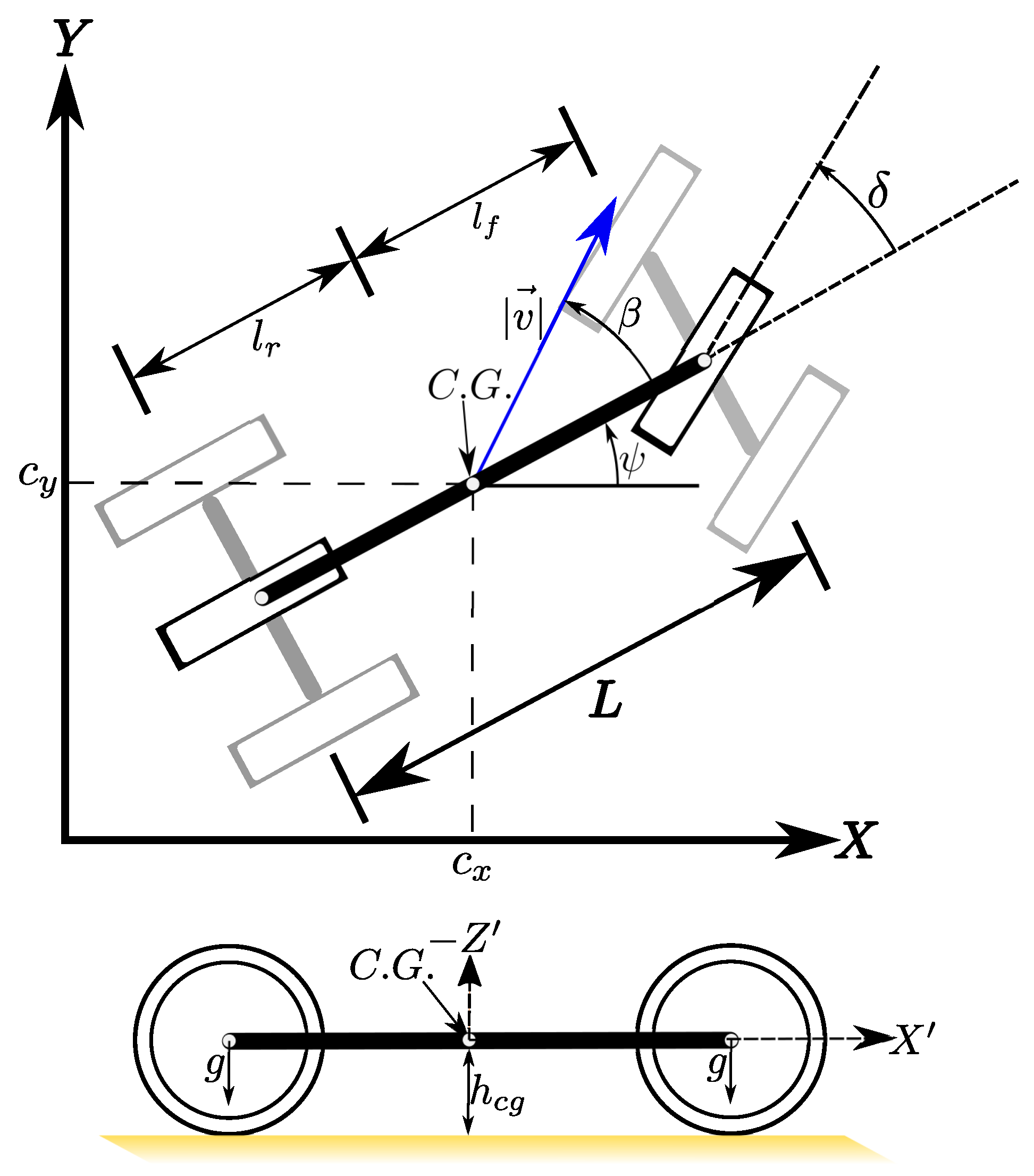
• To represent the load transfer forces generated by the longitudinal acceleration and the effect in the cornering stiffness of the friction coefficient, in this work the Single-Track Model is used. It is necessary to mention that, and with the main aim to develop a manageable mode, restrictions to under- or oversteer, nor driving close to physical capacities of the vehicle were given.
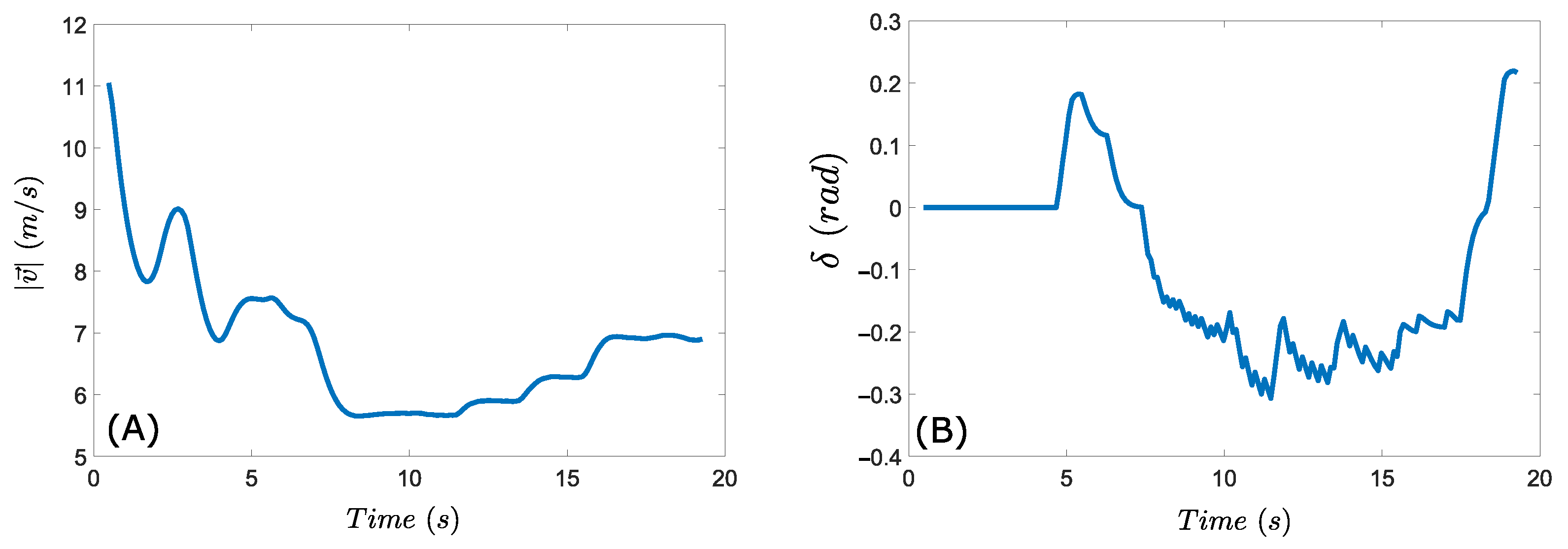
• Numerical results of the proposed VADA obtained in Carla Simulator for different driving scenarios are reported. Results shown that the proposed technique is able to generate a velocity profile and a free-collision trajectory.

The present paper is organized as follows: Section 3 presents the methodology which includes a brief introduction of the ADA approach and the proposed modifications on it for vehicles, the dynamic model of the vehicle, the followed methodology to generate the local path, and the experiments for test the present approach. In Section 4, the results of the given approach are shared, which are followed by a discussion. Finally, the conclusions are given in Section 5.

3. Materials and Methods

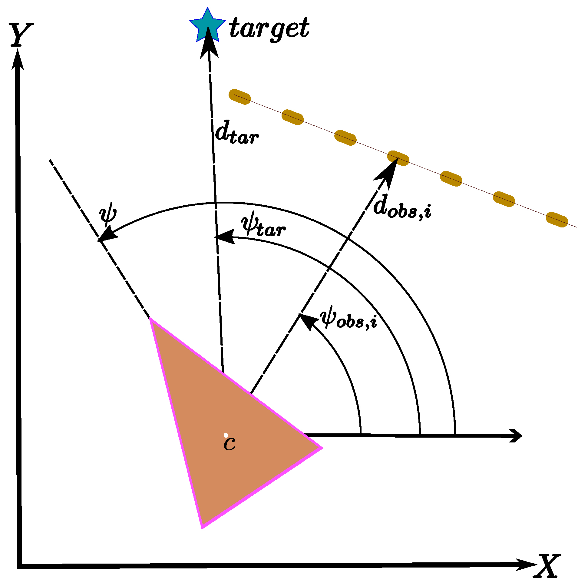
3.1. The Classic Attractor Dynamic Approach

According to Figure 1, there is a target point located at a distance $d_{tar}$ from the vehicle with an initial position c, located in a global coordinates system $XY$. On one hand, the vehicle must reach that target point while avoiding obstacles located at a distance $d_{obs,i}$. On the other hand, there are several critical angles: $\psi$ is the heading angle associated with the vehicle, ${\psi }_{tar}$ is the angle toward the target point and finally, ${\psi }_{obs,i}$ are the angles toward the i-th obstacles.

Just like living beings, to reach a target point, they align their heading directly toward the target and go on to it at a certain speed. If an obstacle is detected, the direction becomes misaligned enough to avoid a collision or likely risk. ADA takes into account this behavior defining two basic objects: attractors and repellers. The set of Equations [44] that describes this behavior are given as follows:

$$\begin{array}{c}\hfill \dot{\psi }=f_{tar}\left(\psi \right)+f_{obs}\left(\psi \right)\end{array}$$

(1)

$$\begin{array}{c}\hfill \dot{v}=v_{tar}\left(v\right)+v_{obs}\left(v\right)\end{array}$$

(2)

Equation (1) represents the rate of change of the heading angle and it is formed by the sum of an attractor $f_{tar}$ and a repeller $f_{obs}$. The attractor is given by Equation (3), where $\psi$ is the heading angle of the vehicle and ${\psi }_{tar}$ is the angle toward the target (see Figure 1) and ${\lambda }_{tar}$ is the maximum strength of the attractor. On the other hand, there is a repeller calculating according to Equation (4), where ${\psi }_{obs,i}$ is the angle toward the i-th of n obstacles, ${\sigma }_i$ is the range of the i-th obstacle and $\tau$ is a parameter that indicates when the repeller is activated regarding to a given distance $d_{obs}$ and ${\lambda }_{obs,i}$ is the maximum strength of the i-th repeller.

$$\begin{array}{ccc}\hfill f_{tar}\left(\psi \right)& =& -{\lambda }_{tar}sin(\psi \left(t\right)-{\psi }_{tar}\left(t\right))\hfill \end{array}$$

(3)

$$\begin{array}{ccc}\hfill f_{obs,i}\left(\psi \right)& =& \sum _{i=1}^n{\lambda }_{obs,i}(\psi \left(t\right)-{\psi }_{obs,i}\left(t\right))exp(-\tau d_{obs,i}\left(t\right))exp\left(-\frac{{(\psi \left(t\right)-{\psi }_{obs,i}\left(t\right))}^2}{2{\sigma }_i^2}\right)\hfill \end{array}$$

(4)

In a similar way, Equation (2) refers to the variation of the velocity $\dot{v}$ and it is formed by an attractor $v_{tar}$ and a repeller $v_{obs}$ of velocity. In this paper, this equation is not considered, due to the change of velocity is calculated in another way as explained in Section 3.4.

3.2. The Attractor Dynamic Approach for Non-Holonomic Vehicles

As mentioned before, the ADA is formed by two mathematic objects: an attractor and a repeller. The space where the vehicle moves is a dynamic system due to it changing over time, under this scheme, an attractor is a function that converges in time to a fixed point in such a system. In the classic ADA, the fixed point is represented as a coordinate in the space; however, such an approach is not suitable for a vehicle due to its non-holonomic characteristics. In addition, the ego-vehicle must converge to the reference path not just to a fixed point. A well-known function that satisfies the requirements of an attractor due it converges exponentially to zero in the desired path, plus taking into account the non-holonomic characteristic of a vehicle, is the mathematical form of Stanley’s Controller [49]. In the core, it is a function that commands the steering input, and therefore, it guides the vehicle to the reference path.

The Stanley controller is given by Equation (5) where $\varphi$ corresponds to the difference between the vehicle and path yaw’s angle, $e_{ct}$ is the cross-track error which is measured from the center of the front axle to the nearest point in the desired path, ${\kappa }_s$ is a gain parameter, $|\overrightarrow{v}|$ is the vehicle velocity, and ${\kappa }_v$ is a term that softening the controller in low velocities. The first term keeps aligned the vehicle to the path, whereas the second term adjust the steering in order to reduce the cross-track error.

$$\begin{array}{ccc}\hfill {\delta }_{att}\left(t\right)& =& \varphi \left(t\right)+{tan}^1\left({\displaystyle \frac{{\kappa }_s{e}_{ct}\left(t\right)}{{\kappa }_v+\left|\overrightarrow{v}\right|\left(t\right)}}\right)\hfill \end{array}$$

(5)

$$\begin{array}{ccc}\hfill \varphi \left(t\right)& =& {\psi }_{path}\left(t\right)-\psi \left(t\right)\hfill \end{array}$$

(6)

On the other hand, the repeller is a point where all the solutions of a given function move away from it. Considering the non-holonomic characteristics of a vehicle and the most common impact angles in a vehicle, it is necessary a function that maximizes the strength of the repeller inside the range of those angles. Such angles, according to [50], are in the range of 10 to 30 degrees considering several ranges of velocity. Moreover, such function must be activated when a repeller is nearby and inhibited when is far. The proposed function is given by Equation (7) where $\lambda$ is the max value that the function could reach, ${\psi }_{obs,i}$ is the angle toward the i-th obstacle, ${\psi }_{max}^{+}$ is the maximum angle to which an obstacle is considered, $d_{obs,i}$ is the current distance toward the i-th obstacle, and $\left|\overrightarrow{v}\right|$ is the vehicle’s speed.

$${\delta }_{rep}\left(t\right)=\sum _{i=1}^n-sgn\left({\psi }_{obs,i}\left(t\right)\right)\lambda {\left(1-{\left|{\displaystyle \frac{{\psi }_{obs,i}\left(t\right)}{{\psi }_{max}^{+}}}\right|}^3\right)}^3\left(2-{\displaystyle \frac{2}{1+exp\left(-{\displaystyle \frac{d_{obs,i}\left(t\right)}{\left|\overrightarrow{v}\right|\left(t\right)}}\right)}}\right)$$

(7)

The tricubic term determines the proportion of lambda in the repeller, further, it takes into account the most common angle of impact by strengthening the repeller through that set, whereas the sigmoid function term determines when an obstacle is activated according to the vehicle’s speed and the distance of the obstacle. Finally, the signum function guarantees that all results move away from the repeller; however, this function is zero when the angle is zero, so in such case, the value of the repeller will be taken as $\lambda$. A plot of the repeller at the negative range of angle and with $\tau =d_{obs}/\left|\overrightarrow{v}\right|$ can be seen in Figure 2. The addition of both terms yields the value of the steering angle as shown in Equation (8). This new form of attractor and repeller is denoted in this work as the vehicle attractor dynamic approach (VADA).

$$\delta \left(t\right)={\delta }_{rep}\left(t\right)+{\delta }_{att}\left(t\right)$$

(8)

It is important to remark that both terms are measured in the vehicle coordinate system $X^{\prime }{Y}^{\prime }$ which is handled according to the norm SAEJ670e (see Figure 3).

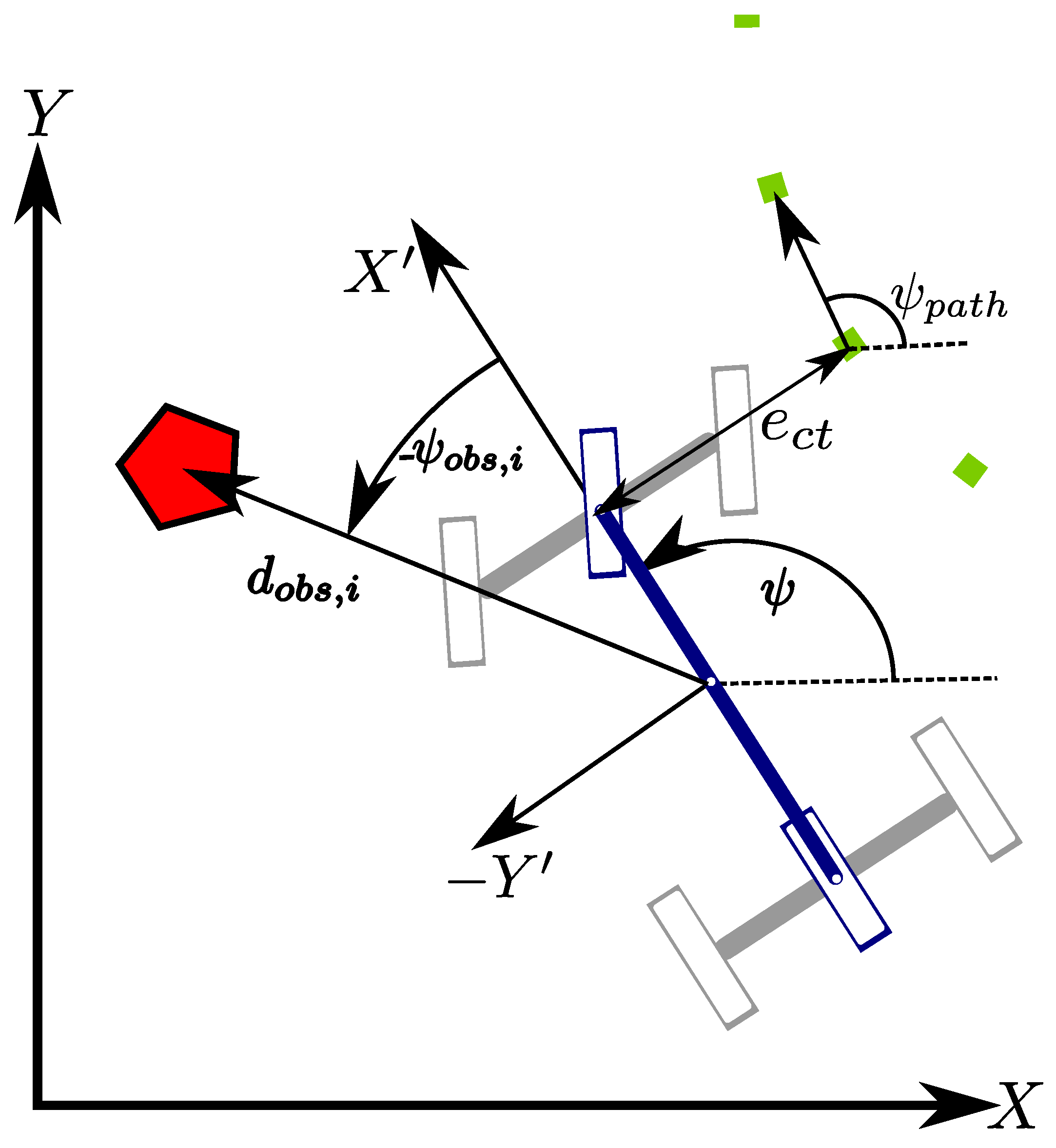
3.3. The Lateral Vehicle Dynamic Model

In order to prove the present approach, the lateral model of the vehicle is mandatory. It is important to remark that the present approach does not take into consideration effects as under- or oversteer, nor driving close to physical capacities of the vehicle. A model that fits under the scope of this approach is the well-known Single-Track Model (ST) whose reference framework can be seen in Figure 4. The ST model used in this paper considers the load transfer forces generated by the longitudinal acceleration and the effect in the cornering stiffness of the friction coefficient. The model was resumed from [51] and its space state is formed by seven degrees of freedom as shown in Equation (9). The control vector is formed by the rate of change of the steering angle and by the longitudinal acceleration as denoted in Equation (10)

$$\begin{array}{ccc}\hfill \overrightarrow{x}& =& {(x_1,x_2,x_3,x_4,x_5,x_6,x_7)}^T={(c_x,c_y,\delta ,\left|\overrightarrow{v}\right|,\psi ,\dot{\psi },\beta )}^T\hfill \end{array}$$

(9)

$$\begin{array}{ccc}\hfill \overrightarrow{u}& =& {(u_1,u_2)}^T={(\dot{\delta },a_x)}^T\hfill \end{array}$$

(10)

Finally, the system is described as follows:

$$\begin{array}{ccc}\hfill {\dot{x}}_1& =& x_{4}cos(x_5+x_7)\hfill \end{array}$$

(11)

$$\begin{array}{ccc}\hfill {\dot{x}}_2& =& x_{4}sin(x_5+x_7)\hfill \end{array}$$

(12)

$$\begin{array}{ccc}\hfill {\dot{x}}_3& =& u_1\hfill \end{array}$$

(13)

$$\begin{array}{ccc}\hfill {\dot{x}}_4& =& u_2\hfill \end{array}$$

(14)

$$\begin{array}{ccc}\hfill {\dot{x}}_5& =& x_6\hfill \end{array}$$

(15)

$$\begin{array}{ccc}\hfill {\dot{x}}_6& =& {\displaystyle \frac{\mu m}{I_z(l_r+l_f)}}(l_f{C}_f{\gamma }_r{x}_3+(l_r{C}_r{\gamma }_f-l_f{C}_f{\gamma }_r)x_7\hfill \\ & & -(l_f^2{C}_f{\gamma }_r+l_r^2{C}_r{\gamma }_f){\displaystyle \frac{x_6}{x_4}})\hfill \end{array}$$

(16)

$$\begin{array}{ccc}\hfill {\dot{x}}_7& =& {\displaystyle \frac{\mu }{x_4(l_r+l_f)}}(C_f{\gamma }_r{x}_3-(C_r{\gamma }_f+C_f{\gamma }_r)x_7\hfill \\ & & +(C_r{\gamma }_f{l}_r-C_f{\gamma }_r{l}_f){\displaystyle \frac{x_6}{x_4}})-x_6\hfill \end{array}$$

(17)

with

$$\begin{array}{ccc}\hfill {\gamma }_r& =& g{l}_r-u_2{h}_{cg}\hfill \end{array}$$

(18)

$$\begin{array}{ccc}\hfill {\gamma }_f& =& g{l}_f+u_2{h}_{cg}\hfill \end{array}$$

(19)

The description for each variable in the model is listed in

Table 1. Nomenclature for the ST vehicle model.

Symbol	Name	Units	Symbol	Name	Units
$c_x$	x position in the XY frame	m	$c_y$	y position in the XY frame	m
$\delta$	Stering angle	rad	$\dot{\delta }$	Rate of change of stering angle	rad/s
$\left|\overrightarrow{v}\right|$	Velocity	m/s	$\psi$	Yaw angle	rad
$\dot{\psi }$	Rate of change of yaw angle	rad/s	$\ddot{\psi }$	Yaw angle acceleration	${\mathrm{rad}/\mathrm{s}}^2$
$\beta$	Side slip angle	rad	$a_x$	Longitudinal acceleration	${\mathrm{m}/\mathrm{s}}^2$
$a_y$	Lateral acceleration	${\mathrm{m}/\mathrm{s}}^2$	g	Gravitational acceleration	${\mathrm{m}/\mathrm{s}}^2$
$\mu$	Friction coefficient	-	m	Mass	kg
$l_f$	Distance of the front tire to C.G.	m	$l_r$	Distance of the rear tire to C.G.	m
$I_z$	Inertia moment on the $Z^{\prime }$ axis	$\mathrm{kg}·{\mathrm{m}}^2$	$C_f$	Cornering stiffness coefficient on the front tire	${\mathrm{rad}}^{-1}$
$C_r$	Cornering stiffness coefficient on the rear tire	${\mathrm{rad}}^{-1}$	$h_{cg}$	Distance of C.G. to ground plane	m

. In addition, some variables are limited according to the capabilities of the vehicle. Equation (21) describes the mechanic ranges for the steering angle. The maximum ranges of acceleration are delimited by Equation (20) whose values were defined according to [52]. The maximum reachable velocity in this work is defined by Equation (22).

$$\begin{array}{ccc}\hfill |a_{min}|\le & |\overrightarrow{a}|& \le |a_{max}|\hfill \end{array}$$

(20)

$$\begin{array}{ccc}\hfill {\delta }_{min}\le & \delta & \le {\delta }_{max}\hfill \end{array}$$

(21)

$$\begin{array}{ccc}\hfill 0\le & |\overrightarrow{v}|& \le |{\overrightarrow{v}}_{max\text{\_}ego}|\hfill \end{array}$$

(22)

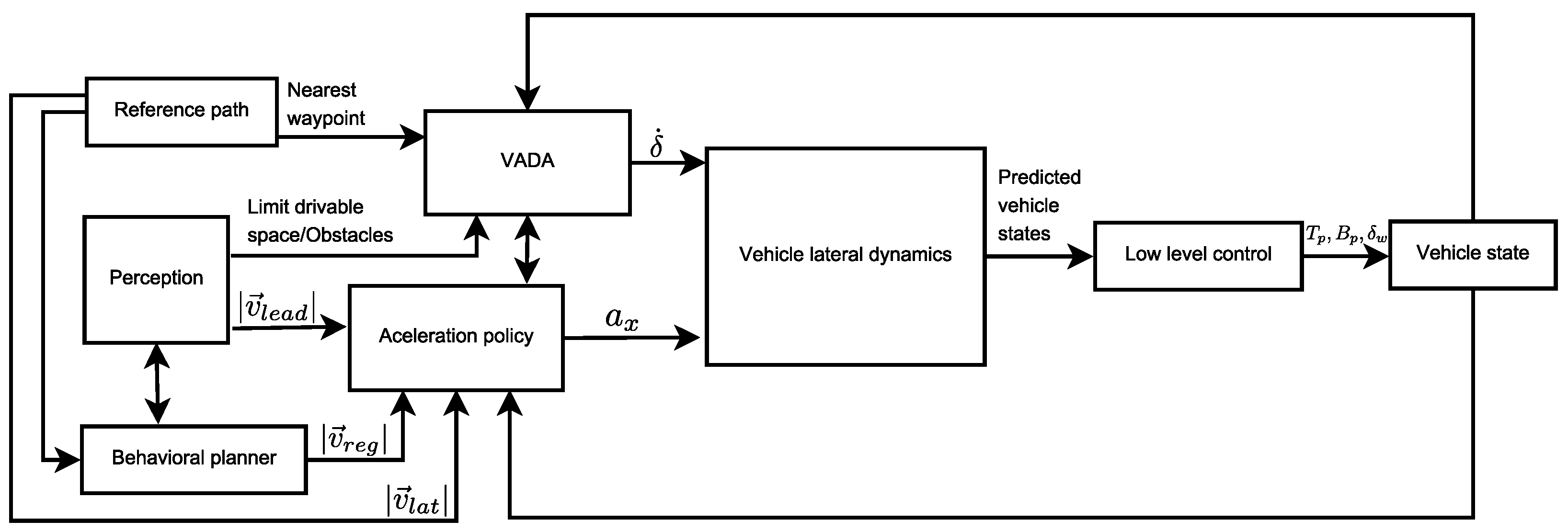
3.4. Local Path Planning Based on VADA

As mentioned before, the local path planning must obtain a free collision trajectory and a velocity profile. In both cases, several constraints regarding safety, comfort, and vehicle dynamics were set. The first constraint is about the maximum speed that the vehicle can reach in a given moment. Such velocity can be sub-divided as follows:

• Maximum curvature velocity$|{\overrightarrow{v}}_{lat}|$: It is the maximum velocity that the ego-vehicle can reach when is driving along a curve. It is delimited by the maximum lateral acceleration $a_{y_{max}}$ and the road’s curvature $\kappa$ as shown in Equation (23)

  $$|{\overrightarrow{v}}_{lat}|={\displaystyle \frac{|a_{y_{max}}|}{\kappa }}$$

  (23)
• Maximum regulatory velocity$|{\overrightarrow{v}}_{reg}|$: It is managed by the regulatory elements of the road such as stop & yield signs, traffic lights, velocity limit signals, among others. The information comes from level (II) of the MP.
• Vehicle leader’s maximum velocity$|{\overrightarrow{v}}_{lead}|$: It is defined as the maximum velocity to keep a constant time gap from a preceding vehicle to the ego-vehicle. Such velocity is determined by integrating a longitudinal desired acceleration which is calculated according to [53].

Once calculated the prior velocities, the maximum allowed one is defined as the minimum of such set as it describes Equation (24)

$$|{\overrightarrow{v}}_{max}|=min(|{\overrightarrow{v}}_{lat}|,|{\overrightarrow{v}}_{reg}|,|{\overrightarrow{v}}_{lead}\left|\right)$$

(24)

Thus, the first constraint is given by Equation (25)

$$|\overrightarrow{v}|\le |{\overrightarrow{v}}_{max}|$$

(25)

The next constraint is about the maximum rate of change of the steering angle. It can be divided into two relationships as shown in Equations (26) and (27). The first one is related to the maximum possible speed of the steering angle $\dot{\delta }$, and the second one constrains the rate of change according to the given velocity $|\overrightarrow{v}|$ and the maximum yaw acceleration $\ddot{\psi }$.

$$\begin{array}{ccc}\hfill |\dot{\delta }|& \le & |{\dot{\delta }}_{max}|\hfill \end{array}$$

(26)

$$\begin{array}{ccc}\hfill |tan(\delta \left(t\right))-tan(\delta (t-dt)\left)\right|& \le & {\displaystyle \frac{|{\ddot{\psi }}_{max}|(l_f+l_r)dt}{|\overrightarrow{v}|}}\hfill \end{array}$$

(27)

The following constraint limits the lateral and longitudinal acceleration under a maximum value whose also limits the wheels into the linear operation zone, such relationships are given by Equations (28) and (29).

$$\begin{array}{ccc}\hfill \sqrt{a_x^2+a_y^2}& \le & |{\overrightarrow{a}}_{max}|\hfill \end{array}$$

(28)

$$\begin{array}{ccc}\hfill a_y& =& |\overrightarrow{v}|\dot{\psi }\hfill \end{array}$$

(29)

A key task for the local path planner is to generate collision-free trajectories. In this work, such a task is performed by the well-known technique of collision circles which consist of setting, at least three circles whose centers are located along the x-axis of the vehicle as can be shown in Figure 5. Once an obstacle is detected, it is analyzed, if a part of the obstacle is inside of the circle, it is considered that a collision occurs in that vehicle position. Thus the last constraint is about the space that the trajectory could reach which is given by Equation (30) where j is the index that corresponds to the given center circle, $R_j$ is the radius of the given circle, i is the index in the set m of given obstacles, and $D_{obs,i}^j$ is the distance of the given i-th obstacle to the given j-th circle’s center. In this work, the mobile obstacles are simplified as cuboids, the dimensions of them are in function of the with of such obstacle, moreover, the drivable zone is also considered as an obstacle and it is represented as points located on its border.

$$\begin{array}{c}\hfill \sum _{i=1}^m(R_j-D_{obs,i}^j)\le 0\\ \hfill jϵ\{r,f,c\}\end{array}$$

(30)

The local path planner, as mentioned before, must deliver to the low-level controller a trajectory and a velocity profile. To perform this task, the Algorithm 1 is proposed where given the current state of the vehicle, obstacles, and drivable limits, a set of points located ahead of the vehicle as well as the corresponding position of the steering angle for each point conforms to the local trajectory. On the other hand, the velocity profile is formed by a set of values of velocity for each point. To calculate both of them, the dynamic model of the vehicle is solved from the current time $t_o$ to a time gap $t_w$.

The outline of the algorithm designed in this paper is shown in Figure 6. The algorithm is divided into four phases, each one characterized by an acceleration policy and by the influence of the VADA. Moreover, it is not mandatory to perform them sequentially since given the situation a phase could be skipped. In the first phase, the exploratory phase, the vehicle calculates its trajectory just by considering the reference path through the attractor and maximum allowed limit velocity. If there is not a risk of collision, the planned path is considered valid. On the other hand, if the vehicle determines a risk of collision for any of the calculated points inside the trajectory, it performed phase two, where the change of velocity is set at maximum values inside the comfort area. If the risk of collision is still present, the next phase is performed by setting the change of velocity above the range of comfort, and the collision points for static obstacles are considered as repellers whereas, for dynamic obstacles, their possible trajectory is calculated and if intersect with the local path generated the current position of the obstacles is considered as repeller. The last phase not just also considers the repellers, but also the deceleration is set as the maximum possible.

Algorithm 1: Local path planning: trajectory and velocity profile generation.

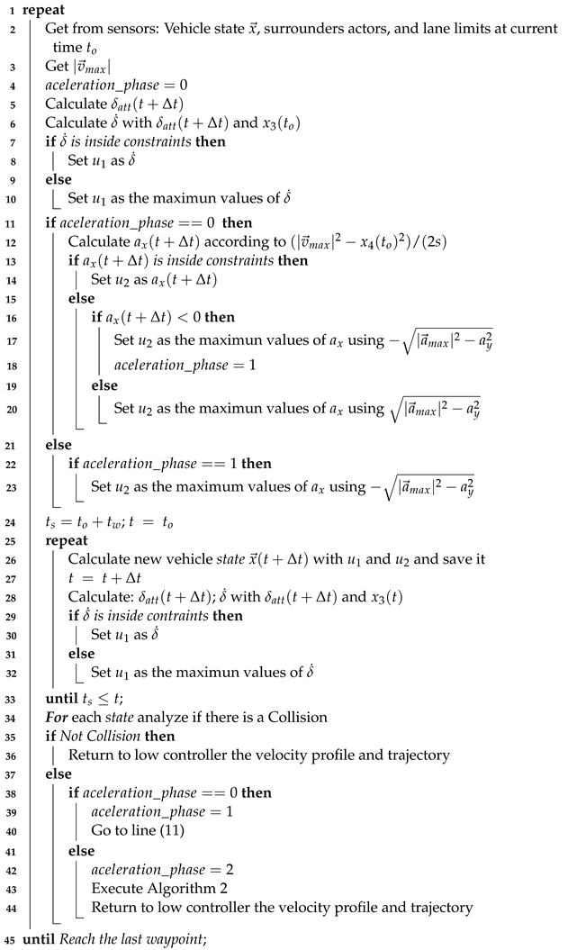
Algorithm 2: Local path planning (Continue).

Since the proposed algorithm is intended to be implemented in real-time scenarios, an analysis of its feasibility in such systems is necessary. One indicator of that is the computational effort needed to be executed which is directly related to the complexity of the algorithm. For the proposed algorithm the computational complexity in the worse scenario is $O(n+m)$ where $n\subseteq m$; on the other hand, the best scenario is $O\left(m\right)$—in other words, when there are no obstacles with risk of a crash. The proposed algorithm runs in linear time and just depends on the number of obstacles to analyze; however, since the analysis of collision from m obstacles does not depend on their past positions. Moreover, the number of states of the local trajectory is fixed, such task could be parallelized in order to enhance the performance of the algorithm. For those reasons, the proposed algorithm may be suitable for applications in real-time. In order to compare the present approach with other algorithms of local path planning, in

Table 2. Computational complexities of some local path planning algorithms.

Reference	Algorithm	Complexity	Marks
[54]	Improved RRT *	$O(alog(a)+b)$	a: Samples
			b: Nodes
[55]	DynEFWA-APF	$O(a+b+cd)$	a: Obstacles
			b: Road marks
			c: Fireworks
			d: Iterations
[40]	APF-ERN	$O(a+ac+bc)$	a: Edges
			b: Nodes
			$c=a+b-1$
Our approach	VADA	$O(n+m)$	n: Collision obstacles
			m: Surrounded obstacles

the computational complexity of similar algorithms is displayed, whereas in

Table 3. Comparison of local path planning algorithms.

Algorithm	Avoidance of Dynamic Obstacles	Reference Path Requierement	Require Smoothing Post-Process	Type of Trajectory
Improved RRT *	No information	Vectorized map	No	Discrete
DynEFWA-APF	✔	Continuous curvature	No	Discrete
APF-ERN	✔	Continuous curvature	Yes	Discrete
VADA	✔	Continuous curvature	No	Discrete
Algorithm	Support technique	Real time	Driving scenario	Reference
Improved RRT *	-	✔	Production	[54]
DynEFWA-APF	Meta-heuristic optimization	✔	Highway	[55]
APF-ERN	Space configuration	✔	Highway	[40]
VADA	Aceleration rules	✔	Highway/Urban	This paper

a set of representative characteristics of local path planners are shown. It is important to remark that this analysis just takes into account the process of generating the local path, in other words, it does not take into account tasks such as the environment interpretation or the prediction of obstacle’s motion due they are not in the scope of this work.

Once we have performed the proposed algorithm, the local path planning is given to the low-level controller. In this work, a PID controller (Equation (31) for the velocity vehicle was used which determines the position of the throttle $T_p$ and brake $B_p$ pedals whose values are normalized in the range of [0, 1]. On the other hand, the steering angle value is correlated with the position of the steering wheel ${\delta }_w$, normalized in the range of [−1, 1], by the linear function ${\delta }_w=c_{\delta }\delta$ where $c_{\delta }$ is a conversion constant. Finally, the values of all constants used in the vehicle dynamic model as well and the VADA are listed in

Table 4. Values and ranges for framework.

Dynamic Model		Constraints		VADA/Control
Symbol	Value	Symbol	Range/Value	Symbol	Range/Value
m	1400	$|\overrightarrow{a}|$	$\left[\right|{\overrightarrow{a}}_{min}|,|{\overrightarrow{a}}_{max}\left|\right]=[-1.8,1.8]$	${\psi }_{max}$	$[{\psi }_{max}^{-},{\psi }_{max}^{+}]=[-2.67,2.67]$
$\mu$	3.5	$|\overrightarrow{v}|$	$[0,|{\overrightarrow{v}}_{max\text{\_}ego}\left|\right]=[0,33]$	$\lambda$	0.4
$l_f$	0.711	$\delta$	$[{\delta }_{min},{\delta }_{max}]=[-1.2,1.2]$	${\kappa }_s$	0.5
$l_r$	1.711	$\dot{\delta }$	$[{\dot{\delta }}_{min},{\dot{\delta }}_{max}]=[-0.4,0.4]$	${\kappa }_v$	3
$C_f$	20.89	$\ddot{\psi }$	$[{\ddot{\psi }}_{min},{\ddot{\psi }}_{max}]=[-2.23,2.23]$	$K_p$	1
$C_r$	20.89	$R_f=R_c=R_r$	1.4	$K_i$	0
$h_{cg}$	0.25	f	1	$K_d$	0.1
g	9.81	c	0	$c_{\delta }$	10/12
$I_z$	1538	r	−1
$∆t$	0.1	$|a_{y_{max}}|$	5.6
$t_w$	2	$a_{brake\_emergency}$	5

.

$$\begin{array}{cc}& u_v=K_p\left(\right|{\overrightarrow{v}}_d|-|\overrightarrow{v}\left|\right)+K_i{\int }_0^t\left(\right|{\overrightarrow{v}}_d|-|\overrightarrow{v}\left|\right)dt+K_d\frac{d\left(\right|{\overrightarrow{v}}_d|-|\overrightarrow{v}\left|\right)}{dt}\\ & T_p=0,B_p=u_{v}if{u}_v<0\\ & T_p=u_v,B_p=0otherwise\end{array}$$

(31)

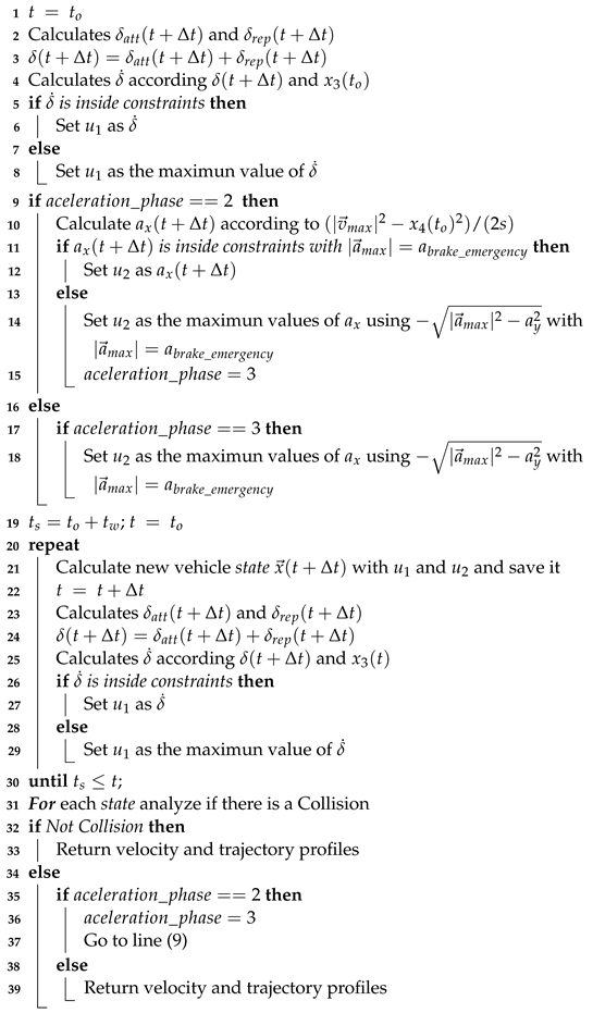
3.5. Path Planning Environment

The use of specialized simulators for autonomous vehicles is a valuable tool for testing the performance, reliability, responses, and behavior of a given new technology. It has become a trend in the automotive industry for many reasons since it allows for improving the quality of testing, safety, and the reduction of costs—to mention just a few. Following this trend, the present approach was tested in a well-known simulator for autonomous vehicles called the Carla Simulator [56] using version 0.9.13 under the o.s Windows 10, executed on a PC with 32 GB of RAM, a Ryzen processor Threadripper 1950x, and a graphic card Radeon 5700 XT. Algorithms 1 and 2 are executed at 10 Hz. When generating the trajectory and velocity profile, the first four states are followed by the low-level controller, and then the path planner is executed again. For reference, in Appendix A, an architecture (see Figure A1) for a real application of the present approach is described.

The cases of study consist of three driving scenarios. The first case (CS1) is about following a preceding vehicle while the ego-vehicle takes a curve. This scenario is important due to the high risk of collision in the event that the ego-vehicle does not adjust its speed or steering in response to the curve or it follows the preceding one too close and therefore is unable to take the curve safely, and as a result, an accident is triggered. This is a basic task for any local path planner. In the second case (CS2) the vehicle must perform an evasive maneuver around a static obstacle. This scenario is representative since vehicles are frequently forced to take evasive action to avoid stationary obstacles, such as stopped vehicles, pedestrians, or debris in the roadway. Finally, in the last scenario (CS3) the vehicle also performs an evasive maneuver but with dynamic obstacles. This scenario is characteristic since many real-world situations, such as avoiding pedestrians in a crowded city street or other cars, require a vehicle to make last-minute changes to its trajectory. In all cases, the local path planner must adjust the steering angle and the velocity to prevent a collision while a reference path is followed.

4. Results and Discussion

It is important to remark that the reference path is settled as a set of waypoints located at the center of the lane and with an approximate separation of 0.2 m between each one. Additionally, the ego-vehicle is denoted by the red car and the borderlines of the drivable space are settled as blue points. The local trajectories are denoted for the colors red, blue, and magenta for the ego-vehicle whereas yellow ones are for the predicted trajectories for surrounding vehicles. The prediction time gap $t_w$ was settled at two seconds in order to force the VADA, and therefore the ego-vehicle, to its limits to planning a secure trajectory and velocity profile.

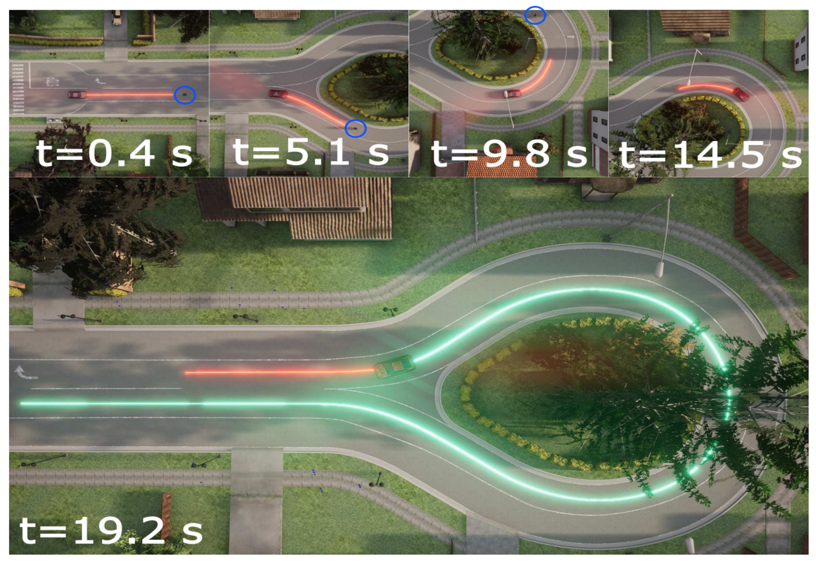
4.1. CS1: Following Reference Global Path, and Velocity Adjust

In this scenario, the vehicle comes with a given speed, and ahead there is a preceding vehicle and a curve path so the ego-vehicle must adjust its velocity and trajectory considering the reference global path, the preceding vehicle velocity, and the maximum curvature velocity. The present scenario is illustrated at different times in Figure 7 whereas both the velocity profile and the steering angle generated along the whole scenario are given in Figure 8.

It is noted that in this case due to there being no collision or risk for the ego-vehicle along the reference path, the influence of the repeller in the command of the steering angle is neglected so the generating of the trajectory is just commanded by the attractor so the problem of local path planning converges to a simple problem of following a reference path with adjusting of velocity. It is observed that the trajectories generated by the algorithm are already dynamically feasible for the vehicle since they are generated by solving the vehicle dynamic model with constraints in a time window. Because this work only focuses on the generation of a local trajectory and a speed profile, the longitudinal model of the vehicle was not taken into account; however, this can be considered by the low-level controller to improve the response of the ego-vehicle which makes the present approach adaptable to different kinds vehicles powertrains.

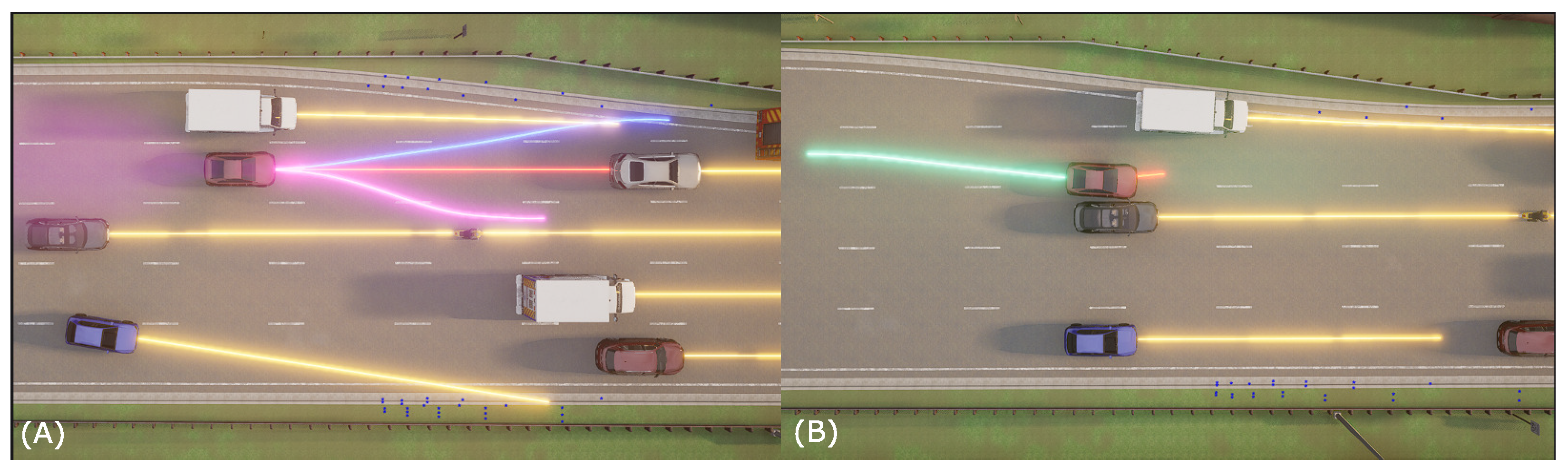
4.2. CS2: Evading a Static Obstacle

In this case, the ego-vehicle was driving at a given speed that represents a risk situation so it must perform an evasive maneuver. As can be seen in Figure 9A the first phase of the path planner algorithm detected a collision in the generated red trajectory. The algorithm determines that the ego-vehicle was driving with a velocity that results in a crash no matter if the velocity is adjusted with the maximum comfort deceleration so the algorithm step to a state where to take into account the repeller(s). In such a state, the blue trajectory was generated which is a free-collision path with a change of velocity inside of comfort parameters as can be seen in Figure 9E and a profile of steering angle displayed in Figure 9D. Due to the scenario being dynamic and the repeller and attractor(s) depending on the velocity and the distance toward the obstacle, naturally, their values change in time. Figure 9B is displayed new trajectories generated after an adjustment of velocity and position of the steering angle. The final trajectory generated is marked in green in Figure 9C where it can be compared with the initially generated trajectories.

It is remarkable that once passed the obstacle, the generated trajectories converge toward the reference path due to the repeller becoming weaker when the angle ${\psi }_{obs}$ converges to ${\psi }_{max}$. It was observed that the present approach was able to plan the trajectory and the speed profile to avoid a collision. Although in this case the first trajectory generated, which takes the repellents into account, was able to select the side from which to avoid the collision (right in this case), the truth is that according to the repellent equation, it becomes uncertain by which side to avoid when the obstacle is exactly in front of the ego vehicle (${\psi }_{obs}\approx 0$). That is why the analysis of collisions and the delimitation of the drivable zone is so important for this approach. The way of the proposed approach overcomes this issue is displayed in the next scenario.

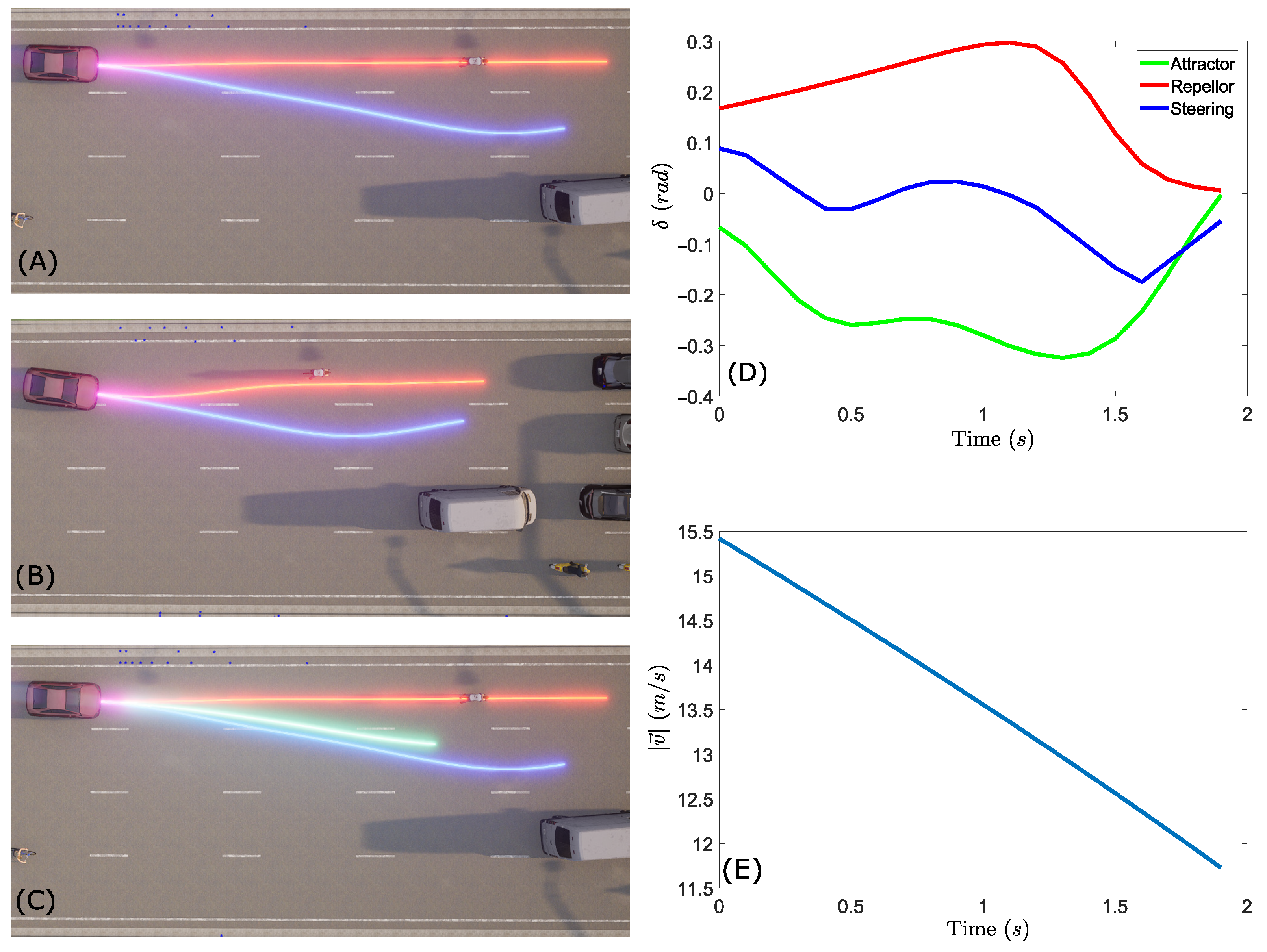
4.3. CS3: Evading Dynamic Obstacles

In this scenario, an adjacent vehicle merges to the current lane of the ego-vehicle whereas around it there are vehicles that also may represent a collision so it must plan a local secure path. According to Figure 10A at first, in the red path, after analyzing the possible trajectories of the surrounded vehicles, two collisions were detected the first one with the preceding vehicle and the second one with the vehicle that will merge with the lane of the ego-vehicle.

The local planner algorithm generates the blue trajectory that is a hardly free collision from the past mentioned vehicles, but the algorithm determines that a collision will be generated with the blue points that delimit the drivable zone so the collision blue points are added to repellers. After that, the algorithm calculates a new path with all repellers which makes the generated trajectory stay within the drivable zone, however, the algorithm determines to decrease the velocity to avoid a collision. The final trajectory can be observed in Figure 10B, although a vehicle passes very close to the ego-vehicle, the local path planner achieves one free-collision plan. The profile of the steering angle for both initial trajectories with repellers are displayed in Figure 11A,B, and the velocities profiles for each trajectory can be seen in Figure 11C, finally the resulting velocity profile across the whole maneuver is displayed in Figure 11D.

One of the limitations of the original ADA is the instability caused due to the temporal evolution of the system when there are many repellers around. At some point, the sum of all the repellers becomes so great that practically the attractor becomes negligible. The original approach seeks to deal with this by inhibiting them (taking into account all surrounding repellers/obstacles); however, in the context of vehicles, and in this work, it was proposed as a way to inhibit the repellers and thus instability, by just taking into account those that represent a risk to the vehicle. As the system evolves over time, different repellers are taken into account only according to the context of the vehicle (possible trajectories), so the problem of instability can be approached from this perspective. The results of the CS3 suggest that this approach can effectively correct the inherent instability of the ADA. On the other hand, the final position of the vehicle may be improved if the time window of prediction is enlarged, which allows the algorithm to plan better paths although it implies increasing the computational effort. For instance, due to the present approach being executed in linear time, by adding one extra second to the time window the computational effort will increase about 50% since the obstacles must be analyzed in that extra time; however, this can be easily approached due to the currently embedded technologies for autonomous vehicles are adapted for performing parallelized tasks and handling large data sets and due to the number of predicted states is handled as a fixed number.

On the other side, it is important to set a metric to evaluate the quality of the generated paths since it allows a further comprehension of the results. The smoothness as a measure of the quality of a path is noteworthy since it is a property that refers to a movement’s continuity or non-intermittency. In other words, it reflects how close the path is to a straight line. This implies that just makes sense to use the smoothness when the path planner generates a trajectory where the $Y^{\prime }$ coordinate changes over time. The smoothness $J_s$ in this work is computed by Equation (32), where N is the total number of nodes of a given trajectory, $c_{y^{\prime }}$ is the lateral position of the node, measured in the $X^{\prime }{Y}^{\prime }$ reference frame, and k is the index of discrete-time.

$$J_s=\frac{1}{N}\sum _{k=1}^{N-1}\left|\right|c_{y^{\prime }}\left(k\right)-c_{y^{\prime }}(k+1)\left|\right|$$

(32)

Given the past equation, the assumption of a maximum value of smoothness given the maximum allowed lateral acceleration to evaluate the generated paths is reasonable. According to the established parameters in Table 4, this value is calculated as 0.5054 m. On the other hand, the smoothness parameter for the planned local path for every studied case is displayed in

Table 5. Generated path smoothness for study cases.

CS1—Figure 7		CS2—Figure 9A,B		CS3—Figure 10A
Reference	Path Smoothness (m)	Reference	Path Smoothness (m)	Reference	Path Smoothness (m)
t = 0.4 (s)	2.50 × ${10}^{-4}$	Red path	0.0643, 0.1495	Red path	0.002
t = 5.1 (s)	0.3264	Blue path	0.1609, 0.1227	Blue path	0.1469
t = 9.8 (s)	0.3891			Magenta path	0.1399
t = 14.5 (s)	0.4327
t = 19.2 (s)	0.3053

. Notice that all values are lower than the maximum permitted one so that the paths can be considered as smooth and dynamically feasible.

On the contrary, there are some drawbacks to the present approach. It should be noted that the algorithm is expected to decelerate when it detects a collision, and this may not be desirable in all cases. In addition to the fact that in the present case studies the reference path does not change throughout the execution of the algorithm the use of a reference path that is always the same may not be realistic in many cases. In particular, in many cases, the reference path may change as a result of changes in the environment. Another aspect to consider is for dynamic objects in which a collision is detected, the location of the repeller is considered static during the local path calculation. This may be appropriate for certain types of dynamic objects, but for others, it may not be. Finally, the present approach just takes into account that the generation of the velocity profile for the ego-vehicle is a ramp one. This assumption is reasonable due to the fact that the change of velocity in a car is a gradual and not sudden process. Considering these limitations, the following factors proposed for study in future research:

• To take into account both accelerations and decelerations to avoid collisions; by choosing the safest option for the ego-vehicle.
• Set a dynamic reference path, for example, when the vehicle generates a trajectory that converges to another lane, in order to change the reference route so that it is established in that lane and thus, the ego-vehicle converges to that lane.
• To move the location of repellers for dynamic obstacles along its predicted trajectory. This would take into account the actual location of the dynamic object at the time of the collision and would adjust the location of the repeller accordingly. This would ensure that the repeller is always in the correct location to avoid the dynamic object. This approach may be more computationally expensive, but it may provide a more accurate collision response.
• It is possible to extend the present work by incorporating other types of velocity profiles.

5. Conclusions

In this article, a new method for local path planning for autonomous vehicles was proposed based on the natural behavior of movement proportioned by the ADA. However, in this work, the original approach was modified in order to adapt it to the vehicle’s non-holonomic constraints taking into account the convergence of the ego-vehicle to a reference path and the avoidance of obstacles, by focusing on the strength of the repellers at the front of the vehicle where the most common crashes angles are located. Those considerations define new attractor and repeller for vehicles and, as the original ADA, the addition of both leads the vehicle to a free obstacle trajectories toward a target. This new form is called VADA. On the other hand, when a person is driving, they follow a reference path under traffic rules and only change their velocity or trajectory when something represents a risk. Following this behavior, the algorithm for local path planning was proposed where the VADA is the core piece along the constraints to generate a velocity profile and a free-collision trajectory.

The results over the present approach suggest that the algorithm could be suitable for starting its implementation in real vehicles due to its performance in numerical simulations and by its complexity which is $O(n+m)$ that is less complex than other algorithms in the state of art. The proposed algorithm was capable of generating collision-free trajectories for a large number of obstacles and dealing with significant changes in the driving environment, such as stopped vehicles and vehicles that join the path of the ego-vehicle—without compromising the safety of the system—demonstrating the viability of the proposed local path planner for real-world applications. In addition, the present approach was capable of generating smooth local paths without the use of post-processes or expensive optimization algorithms compared with other solutions in the state of art. On the other hand, the present approach was capable of overcoming some issues regarding the original ADA. The instability of the system was addressed by reducing the number of repellers. Additionally, the choice of which side the ego-vehicle should choose in order avoid a given obstacle was addressed by adding repellers on the side where the vehicle is not allowed to drive.

References

1. Gkartzonikas, C.; Gkritza, K. What have we learned? A review of stated preference and choice studies on autonomous vehicles. Transp. Res. Part C Emerg. Technol. 2019, 98, 323–337. [Google Scholar] [CrossRef]
2. Yurtsever, E.; Lambert, J.; Carballo, A.; Takeda, K. A survey of autonomous driving: Common practices and emerging technologies. IEEE Access 2020, 8, 58443–58469. [Google Scholar] [CrossRef]
3. Guo, H.; Cao, D.; Chen, H.; Lv, C.; Wang, H.; Yang, S. Vehicle dynamic state estimation: State of the art schemes and perspectives. IEEE/CAA J. Autom. Sin. 2018, 5, 418–431. [Google Scholar] [CrossRef]
4. Musa, A.; Pipicelli, M.; Spano, M.; Tufano, F.; De Nola, F.; Di Blasio, G.; Gimelli, A.; Misul, D.A.; Toscano, G. A Review of Model Predictive Controls Applied to Advanced Driver-Assistance Systems. Energies 2021, 14, 7974. [Google Scholar] [CrossRef]
5. Huang, Z. Application of interval state estimation in vehicle control. Alex. Eng. J. 2022, 61, 911–916. [Google Scholar] [CrossRef]
6. Pendleton, S.D.; Andersen, H.; Du, X.; Shen, X.; Meghjani, M.; Eng, Y.H.; Rus, D.; Ang, M.H. Perception, planning, control, and coordination for autonomous vehicles. Machines 2017, 5, 6. [Google Scholar] [CrossRef]
7. Shi, W.; Alawieh, M.B.; Li, X.; Yu, H. Algorithm and hardware implementation for visual perception system in autonomous vehicle: A survey. Integration 2017, 59, 148–156. [Google Scholar] [CrossRef]
8. Rasouli, A.; Tsotsos, J.K. Autonomous vehicles that interact with pedestrians: A survey of theory and practice. IEEE Trans. Intell. Transp. Syst. 2019, 21, 900–918. [Google Scholar] [CrossRef] [Green Version]
9. Hou, Y.; Wang, C.; Wang, J.; Xue, X.; Zhang, X.L.; Zhu, J.; Wang, D.; Chen, S. Visual Evaluation for Autonomous Driving. IEEE Trans. Vis. Comput. Graph. 2021, 28, 1030–1039. [Google Scholar] [CrossRef]
10. Aradi, S. Survey of deep reinforcement learning for motion planning of autonomous vehicles. IEEE Trans. Intell. Transp. Syst. 2020, 23, 740–759. [Google Scholar] [CrossRef]
11. Lim, W.; Lee, S.; Sunwoo, M.; Jo, K. Hierarchical trajectory planning of an autonomous car based on the integration of a sampling and an optimization method. IEEE Trans. Intell. Transp. Syst. 2018, 19, 613–626. [Google Scholar] [CrossRef]
12. Urmson, C.; Anhalt, J.; Bagnell, D.; Baker, C.; Bittner, R.; Clark, M.; Dolan, J.; Duggins, D.; Galatali, T.; Geyer, C.; et al. Autonomous driving in urban environments: Boss and the urban challenge. J. Field Robot. 2008, 25, 425–466. [Google Scholar] [CrossRef] [Green Version]
13. Soulignac, M. Feasible and optimal path planning in strong current fields. IEEE Trans. Robot. 2010, 27, 89–98. [Google Scholar] [CrossRef]
14. Sánchez-Ibáñez, J.R.; Pérez-del Pulgar, C.J.; García-Cerezo, A. Path Planning for Autonomous Mobile Robots: A Review. Sensors 2021, 21, 7898. [Google Scholar] [CrossRef]
15. Qian, L.; Xu, X.; Zeng, Y.; Li, X.; Sun, Z.; Song, H. Synchronous Maneuver Searching and Trajectory Planning for Autonomous Vehicles In Dynamic Traffic Environments. IEEE Intell. Transp. Syst. Mag. 2020, 14, 57–73. [Google Scholar] [CrossRef] [Green Version]
16. Li, X.; Sun, Z.; Cao, D.; He, Z.; Zhu, Q. Real-time trajectory planning for autonomous urban driving: Framework, algorithms, and verifications. IEEE/ASME Trans. Mechatron. 2015, 21, 740–753. [Google Scholar] [CrossRef]
17. Li, X.; Rosman, G.; Gilitschenski, I.; Araki, B.; Vasile, C.I.; Karaman, S.; Rus, D. Learning an Explainable Trajectory Generator Using the Automaton Generative Network (AGN). IEEE Robot. Autom. Lett. 2021, 7, 984–991. [Google Scholar] [CrossRef]
18. Li, X.; Sun, Z.; Cao, D.; Liu, D.; He, H. Development of a new integrated local trajectory planning and tracking control framework for autonomous ground vehicles. Mech. Syst. Signal Process. 2017, 87, 118–137. [Google Scholar] [CrossRef]
19. Pérez, S.S.; López, J.M.G.; Jimenez Betancourt, R.O.; Villalvazo Laureano, E.; Solís, J.E.M.; Sánchez Cervantes, M.G.; Ochoa Guzmán, V.J. A Low-Cost Platform for Modeling and Controlling the Yaw Dynamics of an Agricultural Tractor to Gain Autonomy. Electronics 2020, 9, 1826. [Google Scholar] [CrossRef]
20. Schöner, G.; Spencer, J. Dynamic Thinking: A Primer on Dynamic Field Theory; Oxford University Press: Oxford, UK, 2016. [Google Scholar]
21. González, D.; Pérez, J.; Milanés, V.; Nashashibi, F. A Review of Motion Planning Techniques for Automated Vehicles. IEEE Trans. Intell. Transp. Syst. 2016, 17, 1135–1145. [Google Scholar] [CrossRef]
22. Claussmann, L.; Revilloud, M.; Gruyer, D.; Glaser, S. A review of motion planning for highway autonomous driving. IEEE Trans. Intell. Transp. Syst. 2019, 21, 1826–1848. [Google Scholar] [CrossRef] [Green Version]
23. Mentasti, S.; Matteucci, M. Multi-layer occupancy grid mapping for autonomous vehicles navigation. In Proceedings of the 2019 AEIT International Conference of Electrical and Electronic Technologies for Automotive (AEIT AUTOMOTIVE), Turin, Italy, 2–4 July 2019; pp. 1–6. [Google Scholar]
24. De Lima, D.A.; Pereira, G.A.S. Navigation of an autonomous car using vector fields and the dynamic window approach. J. Control Autom. Electr. Syst. 2013, 24, 106–116. [Google Scholar] [CrossRef]
25. Sedighi, S.; Nguyen, D.V.; Kapsalas, P.; Kuhnert, K.D. Implementing Voronoi-based Guided Hybrid A* in Global Path Planning for Autonomous Vehicles*. In Proceedings of the 2019 IEEE Intelligent Transportation Systems Conference (ITSC), Auckland, New Zealand, 27–30 October 2019; pp. 3845–3852. [Google Scholar] [CrossRef]
26. Yijing, W.; Zhengxuan, L.; Zhiqiang, Z.; Zheng, L. Local path planning of autonomous vehicles based on A* algorithm with equal-step sampling. In Proceedings of the 2018 37th Chinese Control Conference (CCC), Wuhan, China, 25–27 July 2018; pp. 7828–7833. [Google Scholar]
27. Feraco, S.; Luciani, S.; Bonfitto, A.; Amati, N.; Tonoli, A. A local trajectory planning and control method for autonomous vehicles based on the RRT algorithm. In Proceedings of the 2020 AEIT International Conference of Electrical and Electronic Technologies for Automotive (AEIT AUTOMOTIVE), Turin, Italy, 18–20 November 2020; pp. 1–6. [Google Scholar]
28. Zong, C.; Han, X.; Zhang, D.; Liu, Y.; Zhao, W.; Sun, M. Research on local path planning based on improved RRT algorithm. Proc. Inst. Mech. Eng. Part D J. Automob. Eng. 2021, 235, 2086–2100. [Google Scholar] [CrossRef]
29. Wang, P.; Gao, S.; Li, L.; Sun, B.; Cheng, S. Obstacle avoidance path planning design for autonomous driving vehicles based on an improved artificial potential field algorithm. Energies 2019, 12, 2342. [Google Scholar] [CrossRef] [Green Version]
30. Choi, J.W.; Curry, R.E.; Elkaim, G.H. Continuous Curvature Path Generation Based on Bézier Curves for Autonomous Vehicles. Int. J. Appl. Math. 2010, 40, 2. [Google Scholar]
31. Suzuki, T.; Usami, R.; Maekawa, T. Automatic Two-Lane Path Generation for Autonomous Vehicles Using Quartic B-Spline Curves. IEEE Trans. Intell. Veh. 2018, 3, 547–558. [Google Scholar] [CrossRef]
32. Song, Q.; Zhao, Q.; Wang, S.; Liu, Q.; Chen, X. Dynamic Path Planning for Unmanned Vehicles Based on Fuzzy Logic and Improved Ant Colony Optimization. IEEE Access 2020, 8, 62107–62115. [Google Scholar] [CrossRef]
33. Grigorescu, S.M.; Trasnea, B.; Marina, L.; Vasilcoi, A.; Cocias, T. NeuroTrajectory: A Neuroevolutionary Approach to Local State Trajectory Learning for Autonomous Vehicles. IEEE Robot. Autom. Lett. 2019, 4, 3441–3448. [Google Scholar] [CrossRef] [Green Version]
34. Elsayed, H.; Abdullah, B.A.; Aly, G. Fuzzy logic based collision avoidance system for autonomous navigation vehicle. In Proceedings of the 2018 13th International Conference on Computer Engineering and Systems (ICCES), Cairo, Egypt, 18–19 December 2018; pp. 469–474. [Google Scholar]
35. Hamid, U.Z.A.; Saito, Y.; Zamzuri, H.; Rahman, M.A.A.; Raksincharoensak, P. A review on threat assessment, path planning and path tracking strategies for collision avoidance systems of autonomous vehicles. Int. J. Veh. Auton. Syst. 2018, 14, 134–169. [Google Scholar] [CrossRef]
36. Feraco, S.; Bonfitto, A.; Khan, I.; Amati, N.; Tonoli, A. Optimal Trajectory Generation Using an Improved Probabilistic Road Map Algorithm for Autonomous Driving. Am. Soc. Mech. Eng. 2020, 83938, V004T04A006. [Google Scholar]
37. Fu, M.; Zhang, K.; Yang, Y.; Zhu, H.; Wang, M. Collision-free and kinematically feasible path planning along a reference path for autonomous vehicle. In Proceedings of the 2015 IEEE Intelligent Vehicles Symposium (IV), Seoul, Korea, 28 June–1 July 2015; pp. 907–912. [Google Scholar]
38. Yu, L.; Kong, D.; Shao, X.; Yan, X. A Path Planning and Navigation Control System Design for Driverless Electric Bus. IEEE Access 2018, 6, 53960–53975. [Google Scholar] [CrossRef]
39. Galceran, E.; Eustice, R.M.; Olson, E. Toward integrated motion planning and control using potential fields and torque-based steering actuation for autonomous driving. In Proceedings of the Intelligent Vehicles Symposium (IV), Seoul, Korea, 28 June–1 July 2015; pp. 304–309. [Google Scholar]
40. Huang, Y.; Ding, H.; Zhang, Y.; Wang, H.; Cao, D.; Xu, N.; Hu, C. A motion planning and tracking framework for autonomous vehicles based on artificial potential field elaborated resistance network approach. IEEE Trans. Ind. Electron. 2019, 67, 1376–1386. [Google Scholar] [CrossRef]
41. Snapper, E. Model-Based Path Planning and Control for Autonomous Vehicles Using Artificial Potential Fields. Master’s Thesis, Delft University of Technology, Delft, The Netherlands, 2018. [Google Scholar]
42. Receveur, J.B.; Victor, S.; Melchior, P. Autonomous car decision making and trajectory tracking based on genetic algorithms and fractional potential fields. Intell. Serv. Robot. 2020, 13, 315–330. [Google Scholar] [CrossRef]
43. Schöner, G.; Dose, M. A dynamical systems approach to task-level system integration used to plan and control autonomous vehicle motion. Robot. Auton. Syst. 1992, 10, 253–267. [Google Scholar] [CrossRef]
44. Bicho, E. Dynamic Approach to Behavior-Based Robotics: Design, Specification, Analysis, Simulation and Implementation. Ph.D. Thesis, Universidade do Minho, Braga, Portugal, 2000. [Google Scholar]
45. Bicho, E.; Monteiro, S. Formation control for multiple mobile robots: A non-linear attractor dynamics approach. In Proceedings of the International Conference on Intelligent Robots and Systems, Las Vegas, NV, USA, 8–13 October 2003; Volume 2, pp. 2016–2022. [Google Scholar]
46. Machado, T.; Malheiro, T.; Monteiro, S.; Erlhagen, W.; Bicho, E. Attractor dynamics approach to joint transportation by autonomous robots: Theory, implementation and validation on the factory floor. Auton. Robots 2018, 43, 1–22. [Google Scholar] [CrossRef]
47. Althaus, P.; Ishiguro, H.; Kanda, T.; Miyashita, T.; Christensen, H.I. Navigation for human-robot interaction tasks. In Proceedings of the IEEE International Conference on Robotics and Automation, New Orleans, LA, USA, 26 April–1 May 2004; Volume 2, pp. 1894–1900. [Google Scholar]
48. Hernandes, A.C.; Guerrero, H.B.; Becker, M.; Jokeit, J.S.; Schöner, G. A comparison between reactive potential fields and Attractor Dynamics. In Proceedings of the IEEE 5th Colombian Workshop on Circuits and Systems (CWCAS), Bogota, Colombia, 16–17 October 2014. [Google Scholar]
49. Thrun, S.; Montemerlo, M.; Dahlkamp, H.; Stavens, D.; Aron, A.; Diebel, J.; Fong, P.; Gale, J.; Halpenny, M.; Hoffmann, G.; et al. Stanley: The robot that won the DARPA Grand Challenge. J. Field Robot. 2006, 23, 661–692. [Google Scholar] [CrossRef]
50. Abraham, N.; Ghosh, B.; Simms, C.; Thomson, R.; Amato, G. Assessment of the impact speed and angle conditions for the EN1317 barrier tests. Int. J. Crashworthiness 2016, 21, 211–221. [Google Scholar] [CrossRef] [Green Version]
51. Althoff, M.; Koschi, M.; Manzinger, S. CommonRoad: Composable benchmarks for motion planning on roads. In Proceedings of the 2017 IEEE Intelligent Vehicles Symposium (IV), Los Angeles, CA, USA, 11–14 June 2017; pp. 719–726. [Google Scholar]
52. Bae, I.; Moon, J.; Seo, J. Toward a Comfortable Driving Experience for a Self-Driving Shuttle Bus. Electronics 2019, 8, 943. [Google Scholar] [CrossRef] [Green Version]
53. Fancher, P.; Bareket, Z. Evaluating headway control using range versus range-rate relationships. Veh. Syst. Dyn. 1994, 23, 575–596. [Google Scholar] [CrossRef]
54. Wang, H.; Li, G.; Hou, J.; Chen, L.; Hu, N. A Path Planning Method for Underground Intelligent Vehicles Based on an Improved RRT* Algorithm. Electronics 2022, 11, 294. [Google Scholar] [CrossRef]
55. Li, H.; Liu, W.; Yang, C.; Wang, W.; Qie, T.; Xiang, C. An Optimization-based Path Planning Approach for Autonomous Vehicles using dynEFWA-Artificial Potential Field. IEEE Trans. Intell. Veh. 2021. [Google Scholar] [CrossRef]
56. Dosovitskiy, A.; Ros, G.; Codevilla, F.; Lopez, A.; Koltun, V. CARLA: An open urban driving simulator. In Proceedings of the Conference on Robot Learning, Mountain View, CA, USA, 13–15 November 2017; pp. 1–16. [Google Scholar]
57. Liu, S.; Tang, J.; Zhang, Z.; Gaudiot, J.L. Computer architectures for autonomous driving. Computer 2017, 50, 18–25. [Google Scholar] [CrossRef]
Figure 1. Coordinates systems for ADA.
Energies 15 01769 g001
Figure 2. Characteristic plot of δ r e p for negative values of ψ o b s .
Energies 15 01769 g002
Figure 3. Coordinates systems for the mobile vehicle under the norm SAEJ670e. The coordinate system are placed on the C.G. of the vehicle in order to simplify the present framework.
Energies 15 01769 g003
Figure 4. Reference framework for the ST vehicle model.
Energies 15 01769 g004
Figure 5. Set of secure radius collision-free checker. The center of circles are placed along the X axis.
Energies 15 01769 g005
Figure 6. Flowchart of proposed local path planner.
Energies 15 01769 g006
Figure 7. Generated trajectory at different times. The local path planning is displayed in red, whereas the effective path followed by the ego-vehicle is displayed in green. The preceding vehicle (bicyclist) is marked by a blue circle.
Energies 15 01769 g007
Figure 8. (A) Velocity profile generated along the path. (B) Steering angle calculated by attractor across the reference path.
Energies 15 01769 g008
Figure 9. (A) First frame; (B) second frame; (C) third frame. (D) Resulting steering angle calculated by the influence of the attractor, repellers, and velocity constraints. (E) Velocity profile generated for blue trajectory in the first frame.
Energies 15 01769 g009
Figure 10. (A) Possible generated paths. (B) Final position of ego-vehicle.
Energies 15 01769 g010
Figure 11. (A) Resulting steering angle calculated for blue trajectory. (B) Resulting steering angle calculated for magenta trajectory. (C) Velocity profile for each generated trajectory. (D) Resulting velocity profile for the first to final frame.
Energies 15 01769 g011