
Empirical Modeling of Viscosities and Softening Points of Straight-Run Vacuum Residues from Different Origins and of Hydrocracked Unconverted Vacuum Residues Obtained in Different Conversions

 ,
,  , ,
, ,  ,
,  ,
,  and
and
Abstract
:1. Introduction
2. Materials and Methods
3. Results
3.1. Relations of the Vacuum Residue Properties to Viscosity and Softening Point
3.2. Modeling Straight-Run Vacuum Residue and Hydrocracked Vacuum Residue Viscosity and Softening Point
3.3. Validation of the Developed Models to Simulate Viscosities and Softening Points of SRVRs and H-Oil VTBs
4. Conclusions
- The molecular weight predicted by the correlation of Linan et al. [27] using specific gravity and the T50% boiling point derived from Riazi’s boiling point distribution model for the studied vacuum residues was found to be within the range of molecular weights of distinct vacuum residual oils reported in the literature.
- The ICrA evaluation revealed that the straight-run and hydrocracked (secondary) vacuum residues were completely different, and therefore their viscosities and softening points should be separately modeled.
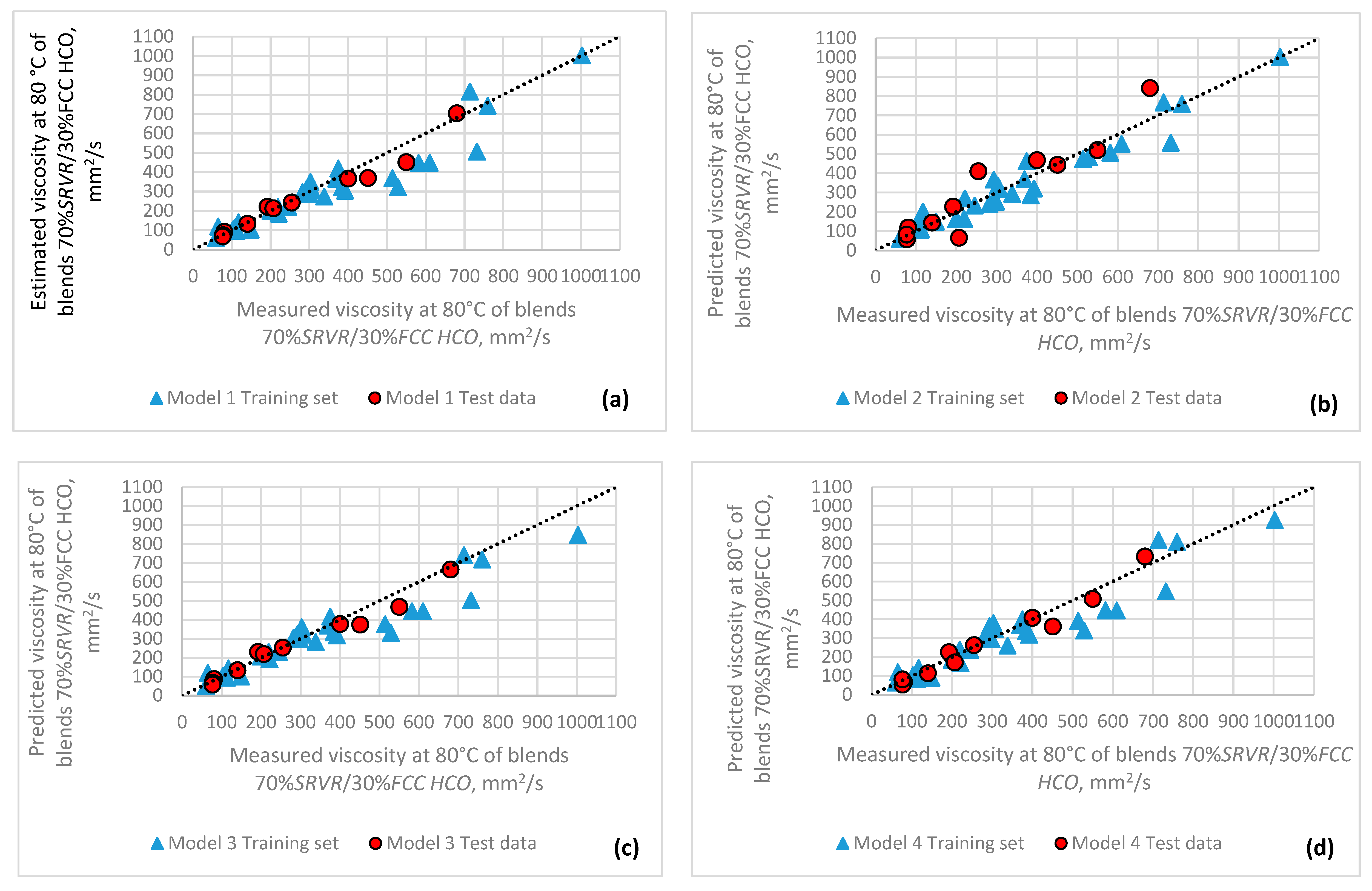
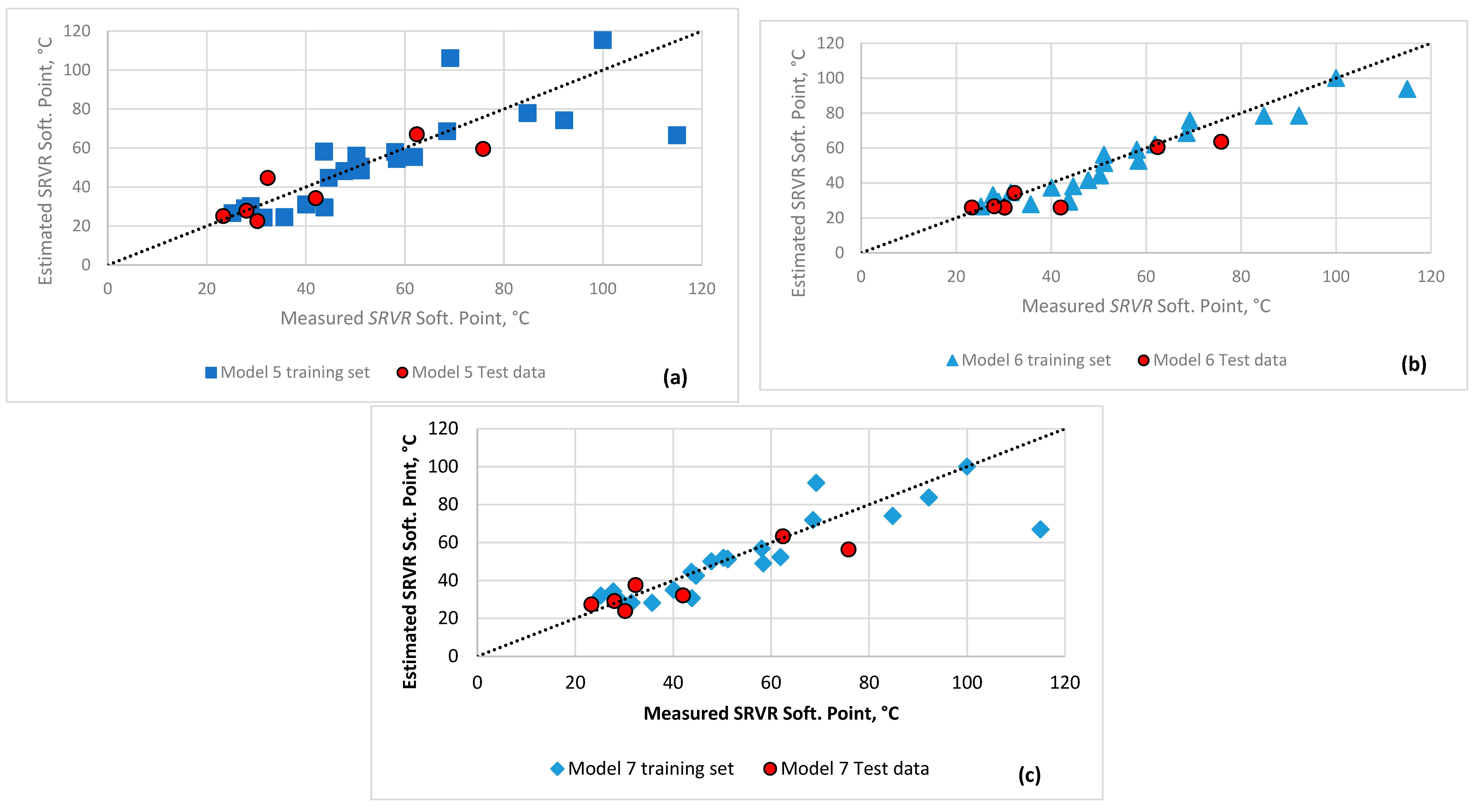
- Both the viscosities and softening points of the primary vacuum residues could be modeled using the properties of T50%, molecular weight, C7-asphaltene content, Conradson carbon content, and specific gravity using a Walther’s-type equation. The best viscosity model employed the molecular weight and specific gravity, whereas the best SRVR softening-point model used the molecular weight and asphaltene content.
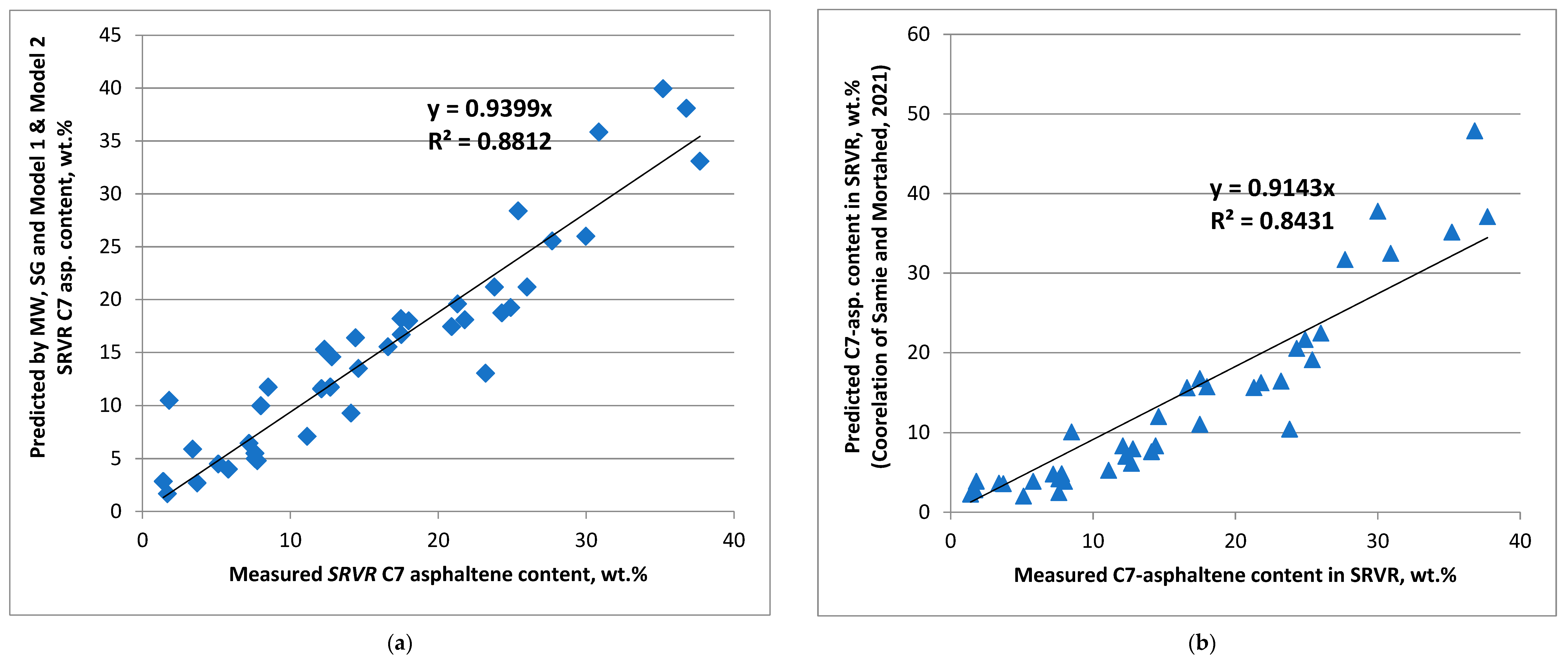
- In addition to the model of Samie and Mortaheb [37], which predicted C7-asphaltene content with an average absolute relative error of 32.6% and used the density, Conradson carbon content, and viscosity of the primary vacuum residue, the C7-asphaltene content could be also predicted from data for density (specific gravity), T50%, and the viscosities in Models 1 and 2 developed in this work, with an average absolute relative error of 20.9%;
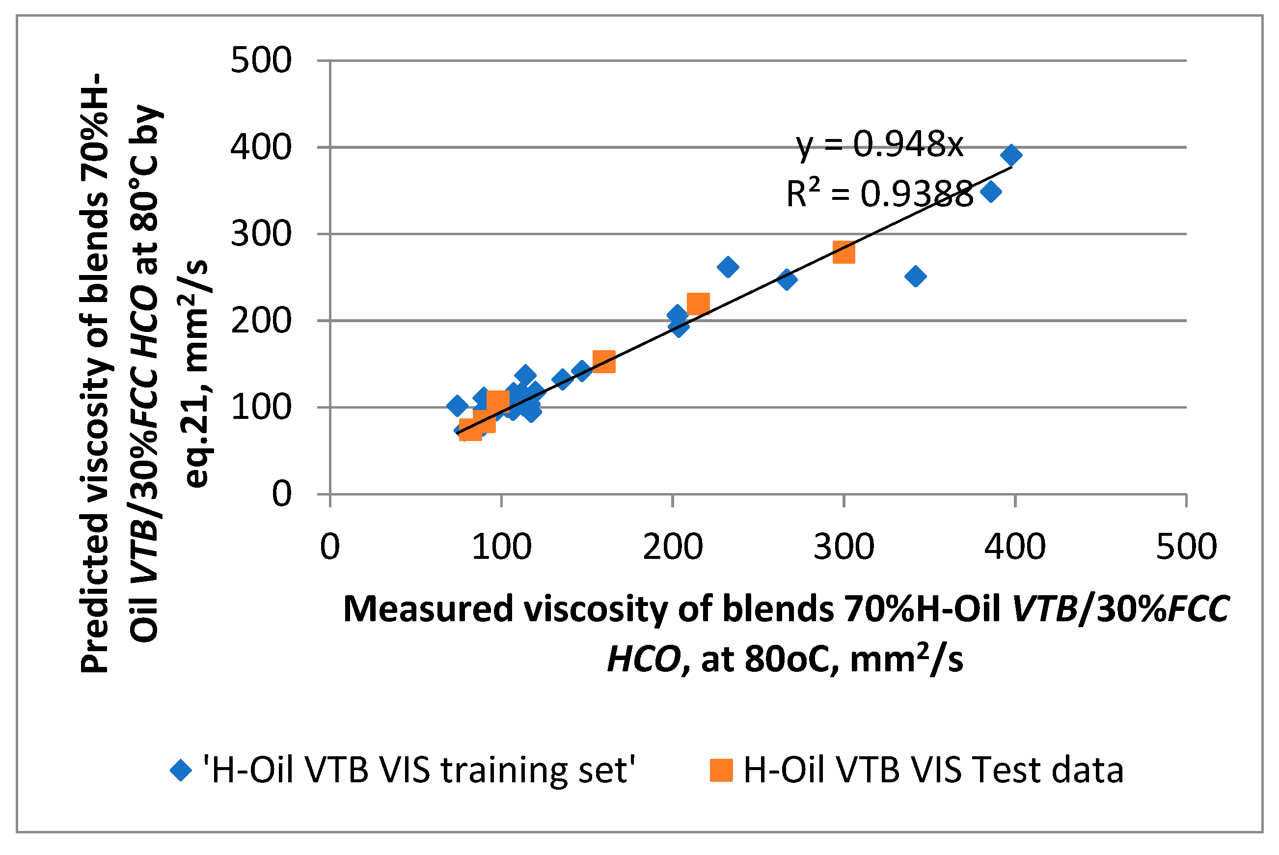
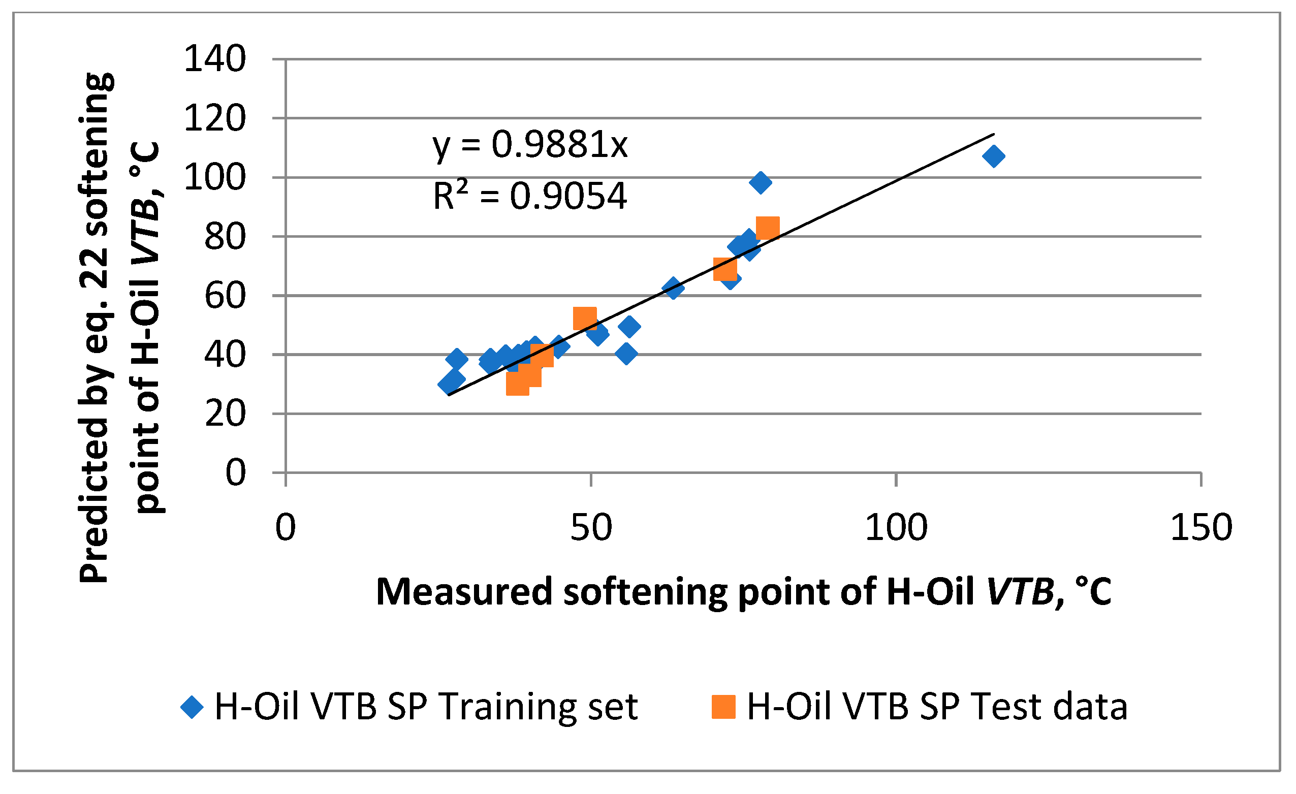
- The viscosities and softening points of the hydrocracked vacuum residues could be modeled from a single property—the Conradson carbon content.
- The vacuum residue viscosity modeled in this research was related to the viscosity of blends of primary and secondary vacuum residue (70%) and FCC HCO (30%) due to the uncertainty of the measurements of viscosities of highly viscous vacuum residua. An investigation of the suitability of blending models available in the literature to the studied blends of vacuum residua (70%) and FCC HCO (30%) to determine the viscosities of the pure primary and secondary vacuum residua will be a subject of a future work.
Supplementary Materials
Author Contributions
Funding
Institutional Review Board Statement
Informed Consent Statement
Data Availability Statement
Acknowledgments
Conflicts of Interest
Nomenclature
| AARE | Average absolute relative error, % |
| ABP | Average boiling point |
| API | API gravity |
| ARI | Aromatic ring index |
| ATB | Atmospheric tower bottom product |
| CCR | Conradson carbon content, wt.% |
| d15 | Density at 15 °C, g/cm3 |
| E | Error |
| FBP | Final boiling point, °C |
| FCC | Fluid catalytic cracking |
| HCO | Heavy cycle oil |
| HNR | Highest number residual |
| ICrA | Intercriteria analysis |
| IBP | Initial boiling point, °C |
| LNB | LUKOIL Neftohim Burgas |
| LNR | Lowest number residual |
| MAX E | Maximum error |
| MIN E | Minimum error |
| MW | Molecular weight, |
| nD20 | Refractive index at 20 °C |
| R | Residual |
| #R+ | Number of positive residuals |
| #R− | Number of negative residuals |
| RSE | Relative standard error |
| SE | Standard error |
| SG | Specific gravity |
| SP | Softening point |
| SRVR | Straight-run vacuum residue |
| SSE | Sum of squared errors |
| VIS | Kinematic viscosity, cSt |
| VR | Vacuum residue |
| VTB | Vacuum tower bottom product |
References
- Stanislaus, A.; Hauser, A.; Marafi, M. Investigation of the mechanism of sediment formation in residual oil hydrocracking process through characterization of sediment deposits. Catal. Today 2005, 109, 167–177. [Google Scholar] [CrossRef]
- Pang, W.-W.; Kuramae, M.; Kinoshita, Y.; Lee, J.-K.; Zhang, Y.Z.; Yoon, S.-H.; Mochida, I. Plugging problems observed in severe hydrocracking of vacuum residue. Fuel 2009, 88, 663–669. [Google Scholar] [CrossRef]
- Stratiev, D.; Dinkov, R.; Shishkova, I.; Sharafutdinov, I.; Ivanova, N.; Mitkova, M.; Yordanov, D.; Rudnev, N.; Stanulov, K.; Artemiev, A.; et al. What is behind the high values of hot filtration test of the ebullated bed residue H-Oil hydrocracker residual oils? Energy Fuels 2016, 30, 7037–7054. [Google Scholar] [CrossRef]
- Miller, K.A.; Nelson, L.A.; Almond, R.M. Should You Trust Your Heavy Oil Viscosity Measurement? J. Can. Pet. Technol. 2006, 45, 42–48. [Google Scholar] [CrossRef]
- Stratiev, D.; Shishkova, I.; Nikolaychuk, E.; Atanasova, V.; Atanassov, K. Investigation of relations of properties of straight run and H-Oil unconverted vacuum residual oils. Pet. Coal 2019, 61, 763–776. [Google Scholar]
- Carbognani, L.; Carbognani-Arambarri, L.; Lopez-Linares, F.; Pereira-Almao, P. Suitable Density Determination for Heavy Hydrocarbons by Solution Pycnometry: Virgin and Thermal Cracked Athabasca Vacuum Residue Fractions. Energy Fuels 2011, 25, 3663–3670. [Google Scholar] [CrossRef]
- Mullins, O.C.; Sheu, E.Y.; Hammami, A.; Marshall, A.G. Asphaltenes, Heavy Oils and Petroleomics; Springer: New York, NY, USA, 2007. [Google Scholar]
- Ruiz-Morales, Y.; Mullins, O.C. Polycyclic aromatic hydrocarbons of asphaltenes analyzed by molecular orbital calculations with optical spectroscopy. Energy Fuels 2007, 21, 256–265. [Google Scholar] [CrossRef]
- Chacón-Patiño, M.L.; Rowland, S.M.; Rodgers, R.P. Advances in asphaltene petroleomics. Part 1: Asphaltenes are composed of abundant island and archipelago structural motifs. Energy Fuels 2017, 31, 13509–13518. [Google Scholar] [CrossRef]
- Chacón-Patiño, M.L.; Rowland, S.M.; Rodgers, R.P. Advances in Asphaltene Petroleomics. Part 2: Selective Separation Method That Reveals Fractions Enriched in Island and Archipelago Structural Motifs by Mass Spectrometry. Energy Fuels 2018, 32, 314–328. [Google Scholar] [CrossRef]
- Chacón-Patiño, M.L.; Rowland, S.M.; Rodgers, R.P. Advances in Asphaltene Petroleomics. Part 3. Dominance of Island or Archipelago Structural Motif Is Sample Dependent. Energy Fuels 2018, 32, 9106–9120. [Google Scholar] [CrossRef]
- Mullins, O.C. The modified Yen model. Energy Fuels 2010, 24, 2179–2207. [Google Scholar] [CrossRef]
- Mullins, O.C.; Sabbah, H.; Eyssautier, J.; Pomerantz, A.E.; Barré, L.; Andrews, A.B.; Ruiz-Morales, Y.; Mostowfi, F.; McFarlane, R.; Goual, L.; et al. Advances in asphaltene science and the Yen—Mullins model. Energy Fuels 2012, 26, 3986–4003. [Google Scholar] [CrossRef]
- Mullins, O.C.; Martinez-Haya, B.; Marshall, A.G. Contrasting perspective on asphaltene molecular weight. this comment vs. the overview of Herod, A.A., Bartle, K.D., Kandiyoti, R. Energy Fuels 2008, 22, 1765–1773. [Google Scholar] [CrossRef]
- Badre, S.; Goncalves, C.C.; Norinaga, K.; Gustavson, G.; Mullins, O.C. Comment on Molecular size and weight of asphaltene and asphaltene solubility fractions from coals, crude oils and bitumen. Fuel 2006, 85, 1950–1951. [Google Scholar] [CrossRef]
- Buch, L.; Groenzin, H.; Buenrostro-Gonzales, E.; Andersen, S.I.; Lira-Galeana, C.; Mullins, O.C. Molecular size of asphaltene fractions obtained from residuum hydrotreatment. Energy Fuels 2003, 82, 1075–1084. [Google Scholar] [CrossRef]
- Wiehe, I.A. A Solvent-Resid Phase Diagram for Tracking Resid Conversion. Ind. Eng. Chem. Res. 1992, 31, 530–536. [Google Scholar] [CrossRef]
- Strausz, O.P.; Safarik, I.; Lown, E.M.; Morales-Izquierdo, A. A critique of asphaltene fluorescence decay and depolarization-based claims about molecular weight and molecular architecture. Energy Fuels 2008, 22, 1156–1166. [Google Scholar] [CrossRef]
- Akbarzadeh, K.; Alboudwarej, H.; Svrcek, W.Y.; Yarranton, H.W. A generalized regular solution model for asphaltene precipitation from n-alkane diluted heavy oils and bitumens. Fluid Phase Equilib. 2005, 232, 159–170. [Google Scholar] [CrossRef]
- Schucker, R.C. Thermogravimetric determination of the coking kinetics of Arab Heavy vacuum residuum. Ind. Eng. Chem. Process Des. Dev. 1983, 22, 615–619. [Google Scholar] [CrossRef]
- Liang, W.; Que, G.; Chen, Y.; Liu, C. Chemical Composition and Characteristics of Residues of Chinese Crude Oils, Asphaltenes and Asphalts. 2. Developments in Petroleum Science; Elsevier Science B.V.: Amsterdam, The Netherlands, 2000. [Google Scholar]
- León, A.Y.; Parra, M.; Grosso, J.L. Estimation of critical properties of typically Colombian vacuum residue SARA fractions. CTF-Cienc. Tecnol. Futuro 2008, 3, 129–142. [Google Scholar]
- Sheremata, J.M.; Gray, M.R.; Dettman, H.D.; McCaffrey, W.C. Quantitative Molecular Representation and Sequential Optimization of Athabasca Asphaltenes. Energy Fuels 2004, 18, 1377–1384. [Google Scholar] [CrossRef]
- Goossens, A.G. Prediction of Molecular Weight of Petroleum Fractions. Ind. Eng. Chem. Res. 1996, 35, 985–988. [Google Scholar] [CrossRef]
- Riazi, M.R.; Daubert, T.E. Characterization Parameters for Petroleum Fractions. Ind. Eng. Chem. Res. 1987, 26, 755–759. [Google Scholar] [CrossRef]
- Riazi, M.R. Characterization and Properties of Petroleum Fraction; ASTM manual series MNL50; ASTM International: Philadelphia, PA, USA, 2005. [Google Scholar]
- Liñan, L.Z.; Lima, N.M.N.; Maciel, M.R.W.; Filho, R.M.; Medina, L.C.; Embiruçu, M. Correlation for predicting the molecular weight of Brazilian petroleum residues and cuts: An application for the simulation of a molecular distillation process. J. Pet. Sci. Eng. 2011, 78, 78–85. [Google Scholar] [CrossRef]
- Stratiev, D.S.; Shishkova, I.K.; Dinkov, R.K.; Petrov, I.P.; Kolev, I.V.; Yordanov, D.; Sotirov, S.; Sotirova, E.; Ribagin, S.; Atanassov, K.; et al. Empirical Models to Characterize the Structural and Physiochemical Properties of Vacuum Gas Oils with Different Saturate Contents. Resources 2021, 10, 71. [Google Scholar] [CrossRef]
- Stratiev, D.S.; Nenov, S.; Shishkova, I.K.; Dinkov, R.K.; Zlatanov, K.; Yordanov, D.; Sotirov, S.; Sotirova, E.; Atanassova, V.; Atanassov, K.; et al. Comparison of Empirical Models to Predict Viscosity of Secondary Vacuum Gas Oils. Resources 2021, 10, 82. [Google Scholar] [CrossRef]
- Liu, Q.; Yang, S.; Liu, Z.; Liu, Q.; Shi, L.; Wei Han, W.; Zhang, L.; Li, M. Comparison of TG-MS and GC-simulated distillation for determination of the boiling point distribution of various oils. Fuel 2021, 301, 121088. [Google Scholar] [CrossRef]
- Carbognani Ortega, L.A.; Carbognani, J.; Pereira Almao, P.P. The Boduszynski Continuum: Contributions to the Understanding of the Molecular Composition of Petroleum Chapter 10. In Correlation of Thermogravimetry and High Temperature Simulated Distillation for Oil Analysis: Thermal Cracking Influence over both Methodologies; American Chemical Society: Washington, DC, USA, 2018; pp. 223–239. [Google Scholar] [CrossRef]
- Stratiev, D.S.; Dinkov, R.K.; Shishkova, I.K.; Nedelchev, A.D.; Tasaneva, T.; Nikolaychuk, E.; Sharafutdinov, I.M.; Rudney, N.; Nenov, S.; Mitkova, M.; et al. An Investigation on the Feasibility of Simulating the Distribution of the Boiling Point and Molecular Weight of Heavy Oils. Pet. Sci. Technol. 2015, 33, 527–541. [Google Scholar] [CrossRef]
- Wiehe, I.A. Asphaltene Solubility and Fluid Compatibility. Energy Fuels 2012, 26, 4004–4016. [Google Scholar] [CrossRef]
- Sánchez-Lemus, M.C.; Okafor, J.C.; Ortiz, D.P.; Schoeggl, F.F.; Taylor, S.D.; van den Berg, F.G.A. Improved density prediction for mixtures of native and refined heavy oil with solvents. Energy Fuels 2015, 29, 3052–3063. [Google Scholar] [CrossRef]
- Sánchez-Lemus, M.C.; Schoeggl, F.; Taylor, S.D.; Yarranton, H.W. Physical properties of heavy oil distillation cuts. Fuel 2016, 180, 457–472. [Google Scholar] [CrossRef]
- Zhao, H.; Memon, A.; Gao, J.; Taylor, S.D.; Sieben, D.; Ratulowski, J.; Alboudwarej, H.; Pappas, J.; Creek, J.L. Heavy Oil Viscosity Measurements—Best Practices and Guidelines. Energy Fuels 2016, 30, 5277–5290. [Google Scholar] [CrossRef]
- Samie, M.S.; Mortaheb, H.R. Novel correlations for prediction of SARA contents of vacuum residues. Fuel 2021, 305, 121609. [Google Scholar] [CrossRef]
- Stratiev, D.; Shishkova, I.; Dinkov, R.; Kirilov, K.; Yordanov, D.; Nikolova, R.; Veli, A.; Tavlieva, M.; Vasilev, S.; Suyunov, R. Variation of oxidation reactivity of straight run and H-Oil hydrocracked vacuum residual oils in the process of road asphalt production. Road Mater. Pavement Des. 2021, 1–25. [Google Scholar] [CrossRef]
- Stratiev, D.; Dinkov, R.; Shishkova, I.; Kirilov, K.; Yordanov, D.; Ilchev, I.; Toteva, V. Laboratory and commercial investigation on the production of road asphalt from blends of straight run and hydrocracked vacuum residua in different ratios. Oxid. Commun. 2021, 44, 652–663. [Google Scholar]
- Stratiev, D.; Shishkova, I.; Nikolaychuk, E.; Ijlstra, W.; Holmes, B.; Caillot, M. Feed properties effect on the performance of vacuum residue ebullated bed H-Oil hydrocracking. Oil Gas Eur. Mag. 2019, 45, 194–200. [Google Scholar]
- Stratiev, D.; Shishkova, I.; Nikolova, R.; Tsaneva, T.; Mitkova, M.; Yordanov, D. Investigation on precision of determination of SARA analysis of vacuum residual oils from different origin. Pet. Coal 2016, 58, 109–119. [Google Scholar]
- Stratiev, D.; Shishkova, I.; Tsaneva, T.; Mitkova, M.; Yordanov, D. Investigation of relations between properties of vacuum residual oils from different origin, and of their deasphalted and asphaltene fractions. Fuel 2016, 170, 115–129. [Google Scholar] [CrossRef]
- Diarov, I.N.; Batueva, I.U.; Sadikov, A.N.; Colodova, N.L. Chemistry of Crude Oil; Chimia Publishers: St. Peterburg, Russia, 1990. (In Russian) [Google Scholar]
- BDS (Bulgarian Standard) EN 1427:2015. Bitumen and Bituminous Binders—Determination of the Softening Point—Ring and Ball Method; BDS: Sofia, Bulgaria, 2015. [Google Scholar]
- Abutaqiya, M. Advances in Thermodynamic Modeling of Nonpolar Hydrocarbons and Asphaltene Precipitation in Crude Oils. Ph.D. Thesis, Rice University, Houston, TX, USA, 2019. [Google Scholar]
- Abutaqiya, M.I.L.; AlHammadi, A.A.; Sisco, C.J.; Vargas, F.M. Aromatic ring index (ARI): A Characterization factor for nonpolar hydrocarbons from molecular weight and refractive index. Energy Fuels 2021, 35, 1113–1119. [Google Scholar] [CrossRef]
- Stratiev, D.S.; Marinov, I.M.; Shishkova, I.K.; Dinkov, R.K.; Stratiev, D.D. Investigation on feasibility to predict the content of saturate plus mono-nuclear aromatic hydrocarbons in vacuum gas oils from bulk properties and empirical correlations. Fuel 2014, 129, 156–162. [Google Scholar] [CrossRef]
- Hernández, E.A.; Sánchez-Reyna, G.; Ancheyta, J. Comparison of mixing rules based on binary interaction parameters for calculating viscosity of crude oil blends. Fuel 2019, 249, 198–205. [Google Scholar] [CrossRef]
- Burnham, K.P.; Anderson, D.R. Model Selection and Multimodel Inference, 2nd ed.; Springer: New York, NY, USA, 2002. [Google Scholar]
- van den Berg, F.G.A.; Heijnis, R.M.A.; Stamps, P.A.; Kramer, P.A. A Geochemical Framework for Understanding Residue Properties. Pet. Sci. Technol. 2003, 21, 449–460. [Google Scholar] [CrossRef]
- Dreillard, M.; Marques, J.; Barbier, J.; Feugnet, F. The Chateaux at Deer Valley. In Proceedings of the Petrophase Conference, Park City, UT, USA, 8–12 July 2018. [Google Scholar]
- Redelius, P.; Soenen, H. Relation between bitumen chemistry and performance. Fuel 2015, 140, 34–43. [Google Scholar] [CrossRef]
- Walther, C. Ueber die Auswertung von Viskosit€atsangaben. Erdoel Teer 1931, 7, 382–384. [Google Scholar]
- Stratiev, D.; Nenov, S.; Nedanovski, D.; Shishkova, I.; Dinkov, R.; Stratiev, D.D.; De Stratiev, D.; Atanassov, K.; Yordanov, D.; Angelova, N.A. Different nonlinear regression techniques and sensitivity analysis as tools to optimize oil viscosity modeling. Resources 2021, 10, 99. [Google Scholar] [CrossRef]
- Stratiev, D.; Nedelchev, A.; Shishkova, I.; Ivanov, A.; Sharafutdinov, I.; Nikolova, R.; Mitkova, M.; Yordanov, D.; Rudnev, N.; Belchev, Z.; et al. Dependence of visbroken residue viscosity and vacuum residue conversion in a commercial visbreaker unit on feedstock quality. Fuel Process. Technol. 2015, 138, 595–604. [Google Scholar] [CrossRef]


| Vacuum Residue and Its SARA Fractions | Minimal Molecular Weight, g/mol | Maximal Molecular Weight, g/mol |
|---|---|---|
| Whole vacuum residue | 581 | 2500 |
| Russia (Akbarzadeh et al., 2005 [19]) | Arab. Heavy (Schucker, 1983 [20]) | |
| Saturates | 361 | 900 |
| Russia (Akbarzadeh et al., 2005 [19]) | Arab. Heavy (Schucker, 1983 [20]) | |
| Aromatics | 450 | 1080 |
| Russia (Akbarzadeh et al., 2005 [19]) | Daqing (Liang et al., 2000 [21]) | |
| Resins | 775 | 1900 |
| Columbian VR2 (León et al., 2008 [22]) | Arab. Heavy (Schucker, 1983 [19]) | |
| Asphaltenes | 750 [7] | 4190 ± 630 |
| Athabasca (Sheremata et al. [23]) |
| Crude Origin | Crude d 15 °C, g/cm3 | Crude Sulfur, % | >540 °C, wt.% | VR SG | VR Concarbon, wt.% | VR Sulfur, % | Sat., wt.% | Aro, wt.% | Res, wt.% | C7-Asp, wt.% | C5-Asp, wt.% | Kin. Vis., mm2/s * | Soft. Point, °C | IBP | 10% | 30% | 50% | 70% | 90% | 95% | FBP | MW | ARI |
|---|---|---|---|---|---|---|---|---|---|---|---|---|---|---|---|---|---|---|---|---|---|---|---|
| Urals | 0.877 | 1.53 | 25.2 | 0.997 | 17.5 | 3.0 | 25.6 | 52.5 | 7.8 | 14.1 | 17.6 | 220.9 | 40.1 | 540 | 559 | 602 | 657 | 735 | 884 | 961 | 1130 | 808 | 4.0 |
| Arab Med. | 0.872 | 2.48 | 25.2 | 1.031 | 20.7 | 5.4 | 11.8 | 68.3 | 5.3 | 14.6 | 25.5 | 338.3 | 44.7 | 538 | 560 | 608 | 670 | 758 | 927 | 1016 | 1217 | 840 | 5.2 |
| Arab Heavy | 0.889 | 2.91 | 32.0 | 1.040 | 23.6 | 5.8 | 12.4 | 61.9 | 4.4 | 21.3 | 32.9 | 374.6 | 51.2 | 538 | 565 | 628 | 709 | 827 | 1060 | 1186 | 1486 | 953 | 5.9 |
| Val’Dagri | 0.832 | 1.97 | 14.6 | 1.052 | 21.4 | 6.0 | 11.7 | 73.5 | 6.4 | 8.5 | 19.5 | 219.3 | 43.7 | 538 | 554 | 593 | 643 | 715 | 857 | 931 | 1086 | 764 | 5.5 |
| Basrah L | 0.878 | 2.85 | 28.3 | 1.052 | 23.8 | 5.9 | 12.3 | 64.8 | 4.9 | 18.0 | 27.7 | 368.9 | 50.3 | 539 | 562 | 616 | 684 | 782 | 969 | 1069 | 1297 | 877 | 6.0 |
| Basrah H | 0.905 | 3.86 | 33.8 | 1.071 | 28.9 | 7.1 | 12.3 | 54.1 | 5.8 | 27.7 | 37.0 | 731.9 | 68.6 | 539 | 567 | 632 | 715 | 836 | 1072 | 1200 | 1504 | 968 | 6.9 |
| Kirkuk | 0.873 | 2.65 | 24.6 | 1.054 | 25.2 | 5.9 | 15.2 | 55.4 | 5.0 | 24.3 | 33.1 | 514.1 | 58.1 | 539 | 561 | 611 | 676 | 769 | 950 | 1046 | 1264 | 853 | 5.9 |
| Iranian H | 0.882 | 2.27 | 28.1 | 1.050 | 23.9 | 5.2 | 17.0 | 52.6 | 5.0 | 25.4 | 36.2 | 528.6 | 61.9 | 540 | 561 | 609 | 668 | 751 | 908 | 989 | 1171 | 832 | 5.7 |
| KEB | 0.876 | 2.64 | 27.7 | 1.037 | 23.3 | 5.7 | 15.0 | 64.2 | 4.2 | 16.6 | 25.7 | 392.3 | 47.8 | 540 | 561 | 608 | 667 | 749 | 901 | 980 | 1157 | 830 | 5.3 |
| El Bouri | 0.891 | 1.76 | 26.2 | 1.050 | 25.5 | 3.3 | 12.0 | 57.9 | 12.6 | 17.5 | 27.3 | 303.0 | 45.0 | 538 | 558 | 605 | 666 | 756 | 931 | 1024 | 1231 | 827 | 5.7 |
| Kazakh H | 0.858 | 0.81 | 23.7 | 0.990 | 17.1 | 1.7 | 33.0 | 50.2 | 5.7 | 11.1 | 17.8 | 117.1 | 27.8 | 539 | 552 | 583 | 621 | 677 | 780 | 832 | 934 | 718 | 3.7 |
| CPC | 0.805 | 0.63 | 9.3 | 0.981 | 16.0 | 2.10 | 44.6 | 40.8 | 10.3 | 3.4 | 11.0 | 65.0 | 25.2 | 538 | 554 | 590 | 637 | 706 | 838 | 906 | 1047 | 757 | 3.5 |
| LSCO | 0.854 | 0.57 | 18.7 | 0.993 | 14.0 | 1.58 | 25.0 | 61.1 | 6.1 | 7.8 | 15.5 | 149.1 | 28.9 | 540 | 554 | 588 | 631 | 692 | 806 | 865 | 984 | 741 | 3.8 |
| Prinos | 0.875 | 3.71 | 20.3 | 1.108 | 32.8 | 9.14 | 12.6 | 50.6 | 6.8 | 30.0 | 38.8 | 550 | 69.2 | 538 | 555 | 595 | 645 | 718 | 858 | 930 | 1085 | 760 | 6.8 |
| SGC | 0.883 | 2.26 | 30.1 | 1.050 | 22.9 | 5.09 | 15.0 | 55.9 | 7.3 | 21.8 | 28.4 | 451 | 58.4 | 540 | 564 | 619 | 689 | 789 | 981 | 1084 | 1319 | 891 | 5.9 |
| Oryx | 0.9156 | 4.209 | 37.4 | 1.089 | 29.4 | 8.01 | 13.3 | 50.1 | 5.7 | 30.9 | 39.6 | 714.0 | 84.8 | 537 | 571 | 653 | 764 | 931 | 1277 | 1473 | 1964 | 1130 | 8.3 |
| Okwuibome | 0.868 | 0.20 | 6.9 | 0.975 | 12.9 | 0.50 | 31.7 | 56.0 | 10.5 | 1.7 | 8.2 | 60.0 | 23.3 | 540 | 549 | 571 | 601 | 643 | 721 | 758 | 818 | 671 | 3.2 |
| Boscan | 1.002 | 5.50 | 63.1 | 1.078 | 27.8 | 6.00 | 15.1 | 44.5 | 5.3 | 35.2 | 41.0 | 1003.0 | 115.0 | 542 | 588 | 689 | 812 | 982 | 1295 | 1459 | 1841 | 1330 | 8.7 |
| RasGharib | 0.926 | 3.44 | 40.2 | 1.059 | 25.1 | 5.60 | 14.7 | 49.7 | 9.6 | 26.0 | 34.9 | 610.0 | 75.8 | 540 | 567 | 628 | 706 | 814 | 1020 | 1128 | 1383 | 940 | 6.4 |
| Varandey | 0.850 | 0.63 | 14.9 | 0.990 | 15.1 | 1.70 | 33.5 | 47.6 | 11.3 | 7.6 | 13.5 | 103.0 | 43.8 | 539 | 552 | 582 | 621 | 677 | 783 | 837 | 942 | 717 | 3.7 |
| Albania | 1.001 | 5.64 | 48.2 | 1.094 | 31.4 | 8.70 | 10.0 | 52.9 | 6.3 | 37.7 | 49.7 | 680.0 | 92.2 | 540 | 572 | 645 | 732 | 850 | 1061 | 1166 | 1388 | 1017 | 7.9 |
| Tempa Rossa | 0.940 | 5.35 | 37.6 | 1.120 | 34.3 | 9.3 | 2.2 | 48.4 | 12.6 | 36.8 | 46.8 | 759.5 | 100.0 | 540 | 568 | 630 | 708 | 816 | 1021 | 1129 | 1383 | 931 | 8.2 |
| Forties | 0.817 | 0.68 | 11.9 | 0.990 | 14.8 | 2.5 | 28.7 | 60.3 | 3.8 | 7.2 | 9.8 | 140.0 | 28.9 | 541 | 557 | 594 | 643 | 716 | 858 | 932 | 1081 | 772 | 3.8 |
| Rhemoura | 0.865 | 0.75 | 20.2 | 1.041 | 23.7 | 1.8 | 19.7 | 49.8 | 7.3 | 23.2 | 31.3 | 255 | 51.1 | 538 | 555 | 593 | 642 | 713 | 846 | 916 | 1063 | 766 | 5.2 |
| Cheleken | 0.847 | 0.40 | 16.6 | 0.974 | 12.3 | 1.2 | 34.2 | 51.8 | 8.2 | 5.8 | 12.5 | 81 | 35.7 | 541 | 556 | 589 | 632 | 694 | 810 | 869 | 989 | 745 | 3.2 |
| Arab Light | 0.858 | 1.89 | 22.9 | 1.029 | 18.7 | 4.9 | 15.9 | 64.7 | 7.3 | 12.1 | 18.8 | 192 | 32.3 | 540 | 558 | 597 | 647 | 716 | 843 | 908 | 1049 | 778 | 4.9 |
| Azeri Light | 0.848 | 0.20 | 14.8 | 0.967 | 9.5 | 0.5 | 40.2 | 50.1 | 8.4 | 1.4 | 5.4 | 77 | 30.2 | 539 | 553 | 585 | 627 | 686 | 799 | 856 | 971 | 731 | 3.0 |
| Aseng | 0.874 | 0.26 | 13.8 | 0.984 | 14.2 | 0.6 | 32.7 | 48.5 | 15.2 | 3.7 | 10.0 | 77 | 28.0 | 541 | 549 | 569 | 595 | 630 | 694 | 723 | 776 | 658 | 3.4 |
| Buzachi | 0.907 | 1.57 | 32.7 | 1.007 | 16.0 | 3.1 | 25.0 | 67.4 | 5.8 | 1.8 | 6.1 | 207 | 38.0 | 542 | 562 | 610 | 672 | 761 | 934 | 1025 | 1227 | 848 | 4.4 |
| KBT | 0.876 | 2.91 | 25.8 | 1.067 | 26.9 | 6.4 | 12.3 | 53.6 | 9.2 | 24.9 | 32.4 | 400 | 62.4 | 540 | 560 | 607 | 665 | 749 | 907 | 990 | 1174 | 821 | 6.2 |
| No. | H-Oil Conv., wt.% | H-Oil VTB SG | H-Oil VTB CCR | Sat., wt.% | Aro, wt.% | Res, wt.% | C7-Asp, wt.% | C5-Asp, wt.% | Kin. Vis., mm2/s | Soft. Point, °C | IBP | 10% | 30% | 50% | 70% | 90% | 95% | FBP | MW | ARI |
|---|---|---|---|---|---|---|---|---|---|---|---|---|---|---|---|---|---|---|---|---|
| 1 | 75 | 1.006 | 21.8 | 26.4 | 53.7 | 9.7 | 10.1 | 21.0 | 90.7 | 37.8 | 541 | 551 | 573 | 598 | 629 | 679 | 702 | 744 | 663 | 4.0 |
| 2 | 69 | 1.011 | 22.6 | 25.6 | 56.4 | 11.2 | 6.8 | 26.4 | 106.7 | 38.4 | 541 | 552 | 574 | 599 | 631 | 680 | 703 | 744 | 666 | 4.1 |
| 3 | 70 | 1.021 | 23.4 | 23.8 | 48.9 | 11.9 | 15.4 | 26.0 | 112.8 | 37.5 | 541 | 551 | 573 | 597 | 628 | 677 | 700 | 741 | 661 | 4.4 |
| 4 | 75 | 1.021 | 24.1 | 23.9 | 48.8 | 12.8 | 14.5 | 27.0 | 103.1 | 38.1 | 541 | 551 | 574 | 599 | 631 | 683 | 706 | 750 | 665 | 4.4 |
| 5 | 65 | 1.025 | 23.6 | 23.3 | 51.2 | 9.4 | 16.1 | 23.6 | 103.7 | 41.3 | 539 | 550 | 572 | 597 | 629 | 681 | 704 | 749 | 661 | 4.4 |
| 6 | 64 | 1.015 | 22.1 | 24.8 | 49.0 | 10.9 | 15.3 | 24.9 | 117.2 | 37.9 | 539 | 550 | 572 | 596 | 628 | 677 | 700 | 742 | 660 | 4.2 |
| 7 | 59 | 1.002 | 19.1 | 27.4 | 48.6 | 13.2 | 10.8 | 25.5 | 89.2 | 27.6 | 540 | 551 | 574 | 600 | 631 | 682 | 704 | 748 | 668 | 3.9 |
| 8 | 68 | 1.026 | 23.6 | 23.1 | 48.7 | 11.8 | 16.4 | 26.0 | 116.4 | 41.0 | 539 | 550 | 572 | 598 | 631 | 684 | 708 | 753 | 662 | 4.5 |
| 9 | 73 | 1.036 | 24.0 | 21.7 | 49.9 | 13.9 | 14.5 | 28.5 | 114.7 | 36.0 | 540 | 550 | 572 | 597 | 629 | 681 | 705 | 748 | 659 | 4.7 |
| 10 | 67 | 1.029 | 23.1 | 22.6 | 47.5 | 15.2 | 14.7 | 28.6 | 103.3 | 38.5 | 540 | 552 | 577 | 604 | 638 | 691 | 715 | 763 | 676 | 4.6 |
| 11 | 61.3 | 1.009 | 22.5 | 25.9 | 43.1 | 12.8 | 18.2 | 28.9 | 89.6 | 40.7 | 539 | 553 | 581 | 610 | 645 | 700 | 724 | 774 | 691 | 4.1 |
| 12 | 62.0 | 1.016 | 22.5 | 24.6 | 48.8 | 15.9 | 10.7 | 27.7 | 106.6 | 37.4 | 541 | 553 | 579 | 609 | 645 | 703 | 730 | 783 | 687 | 4.3 |
| 13 | 55.3 | 0.9860 | 17.9 | 31.1 | 43.3 | 9.8 | 15.7 | 24.5 | 78.4 | 26.7 | 541 | 552 | 575 | 601 | 633 | 684 | 706 | 749 | 671 | 3.5 |
| 14 | 72.3 | 1.027 | 24.7 | 22.9 | 48.7 | 10.7 | 17.7 | 27.4 | 89.6 | 39.4 | 541 | 554 | 580 | 609 | 643 | 699 | 724 | 773 | 686 | 4.6 |
| 15 | 67.4 | 1.020 | 23.3 | 23.9 | 51.2 | 8.5 | 16.4 | 25.4 | 96.5 | 33.5 | 540 | 551 | 574 | 599 | 631 | 682 | 704 | 748 | 665 | 4.3 |
| 16 | 65.8 | 1.013 | 22.4 | 25.2 | 49.9 | 14.7 | 10.2 | 26.3 | 90.2 | 33.5 | 539 | 550 | 573 | 598 | 630 | 679 | 702 | 744 | 664 | 4.2 |
| 17 | 64.9 | 1.018 | 23.3 | 24.3 | 48.7 | 11.5 | 15.4 | 24.4 | 74.2 | 28.0 | 540 | 551 | 575 | 601 | 634 | 684 | 707 | 751 | 670 | 4.3 |
| 18 | 72.5 | 1.034 | 25.5 | 22.0 | 50.7 | 10.2 | 17.2 | 25.8 | 107 | 40.85 | 541 | 551 | 574 | 599 | 632 | 686 | 710 | 756 | 664 | 4.7 |
| 19 | 75.3 | 1.042 | 25.5 | 21.0 | 49.8 | 10.7 | 18.5 | 28.5 | 111.7 | 44.6 | 541 | 551 | 573 | 598 | 632 | 688 | 713 | 761 | 662 | 4.8 |
| 20 | 81.2 | 1.056 | 28.2 | 19.6 | 54.2 | 6.2 | 20.0 | 23.1 | 113.9 | 50.9 | 539 | 549 | 570 | 594 | 626 | 678 | 701 | 744 | 651 | 5.1 |
| 21 | 71.6 | 1.030 | 24.4 | 22.5 | 50.8 | 5.4 | 21.3 | 26.0 | 109.9 | 55.8 | 540 | 550 | 570 | 594 | 624 | 673 | 694 | 734 | 653 | 4.5 |
| 22 | 74.3 | 1.059 | 28.8 | 19.3 | 52.0 | 5.9 | 22.8 | 27.5 | 147.0 | 56.3 | 541 | 550 | 571 | 595 | 627 | 678 | 702 | 744 | 653 | 5.2 |
| 23 | 71.7 | 1.036 | 25.7 | 21.6 | 52.4 | 4.5 | 21.4 | 24.2 | 119.7 | 44.7 | 541 | 551 | 573 | 599 | 634 | 691 | 718 | 767 | 664 | 4.7 |
| 24 | 75.7 | 1.050 | 27.6 | 20.1 | 51.8 | 15.2 | 12.9 | 29.8 | 135.7 | 51.1 | 541 | 551 | 572 | 596 | 628 | 679 | 702 | 744 | 656 | 5.0 |
| 25 | 67.0 | 1.009 | 22.2 | 25.9 | 50.8 | 8.7 | 14.6 | 21.9 | 95.5 | 37.8 | 540 | 551 | 573 | 598 | 630 | 680 | 702 | 745 | 664 | 4.1 |
| 26 | 68.9 | 1.022 | 22.4 | 23.6 | 51.8 | 8.2 | 16.4 | 24.0 | 97.0 | 38.5 | 539 | 550 | 572 | 598 | 630 | 683 | 706 | 751 | 663 | 4.4 |
| 27 | 87.5 | 1.148 | 45.6 | 4.0 | 6.3 | 22.7 | 67.0 | 91.0 | 397.8 | 116.0 | 540 | 552 | 577 | 605 | 640 | 694 | 719 | 768 | 656 | 6.9 |
| 28 | 90.1 | 1.103 | 38 | 16.6 | 39.1 | 12.9 | 31.4 | 44.1 | 266.5 | 76 | 540 | 549 | 569 | 593 | 624 | 675 | 698 | 737 | 640 | 6.0 |
| 29 | 93.2 | 1.094 | 35.0 | 17.0 | 34.9 | 16.1 | 32.0 | 47.1 | 202.8 | 72.8 | 541 | 550 | 569 | 591 | 622 | 671 | 693 | 729 | 638 | 5.8 |
| 30 | 93.1 | 1.125 | 43.7 | 15.8 | 24.1 | 13.4 | 46.7 | 53.9 | 385.8 | 77.8 | 541 | 550 | 569 | 591 | 621 | 671 | 693 | 729 | 632 | 6.3 |
| 31 | 93 | 1.098 | 33.9 | 16.8 | 36.8 | 10.9 | 35.5 | 45.4 | 203.6 | 63.5 | 539 | 547 | 567 | 590 | 620 | 668 | 690 | 728 | 634 | 5.9 |
| 32 | 83.9 | 1.136 | 38.95 | 15.5 | 40.4 | 13.4 | 30.7 | 42.9 | 232.3 | 75.9 | 540 | 550 | 570 | 594 | 625 | 676 | 698 | 737 | 635 | 6.6 |
| 33 | 83.6 | 1.122 | 38.26 | 15.8 | 45.0 | 11.9 | 27.3 | 38.6 | 341.9 | 74.2 | 541 | 549 | 567 | 589 | 617 | 664 | 685 | 718 | 627 | 6 |
| SRVR | H-Oil VTB | |||
|---|---|---|---|---|
| Min. | Max | Min. | Max | |
| SG | 0.967 | 1.120 | 0.986 | 1.148 |
| Conradson carbon content, wt.% | 9.5 | 34.3 | 17.9 | 45.6 |
| Saturates, wt.% | 2.2 | 44.6 | 4.0 | 31.1 |
| Aromatics, wt.% | 40.8 | 73.5 | 6.3 | 56.4 |
| Resins, wt.% | 3.8 | 15.2 | 4.5 | 22.7 |
| C7-asphaltenes, wt.% | 1.4 | 37.7 | 6.8 | 67.0 |
| C5-asphaltenes, wt.% | 5.4 | 49.7 | 21.0 | 91.0 |
| Molecular weight, g/mol | 658 | 1330 | 627 | 691 |
| Kin. viscosity of the blends of 70%VR/30%FCCHCO, mm2/s | 60 | 1003 | 74 | 398 |
| Softening point, °C | 23.3 | 115 | 27 | 116 |
| Aromatic ring index | 3.0 | 8.7 | 3.5 | 6.9 |
| Crude d15 | Crude S | VR | VR SG | VR CCR | VR S | Sat | Aro | Res | C7-Asp | C5-Asp | VIS | SP | T50% | MW | ARI | |
|---|---|---|---|---|---|---|---|---|---|---|---|---|---|---|---|---|
| Crude d15 | 1.000 | 0.777 | 0.903 | 0.756 | 0.766 | 0.708 | 0.267 | 0.467 | 0.453 | 0.789 | 0.777 | 0.768 | 0.766 | 0.805 | 0.800 | 0.784 |
| Crude S | 0.777 | 1.000 | 0.828 | 0.885 | 0.887 | 0.922 | 0.191 | 0.490 | 0.359 | 0.885 | 0.885 | 0.874 | 0.812 | 0.855 | 0.846 | 0.917 |
| VR | 0.903 | 0.828 | 1.000 | 0.772 | 0.763 | 0.754 | 0.271 | 0.508 | 0.384 | 0.818 | 0.807 | 0.807 | 0.777 | 0.878 | 0.878 | 0.809 |
| VR SG | 0.756 | 0.885 | 0.772 | 1.000 | 0.924 | 0.899 | 0.154 | 0.476 | 0.425 | 0.897 | 0.881 | 0.876 | 0.814 | 0.789 | 0.775 | 0.929 |
| VR CCR | 0.766 | 0.887 | 0.763 | 0.924 | 1.000 | 0.885 | 0.195 | 0.451 | 0.439 | 0.901 | 0.899 | 0.864 | 0.805 | 0.775 | 0.770 | 0.894 |
| VR S | 0.708 | 0.922 | 0.754 | 0.899 | 0.885 | 1.000 | 0.161 | 0.520 | 0.386 | 0.835 | 0.832 | 0.823 | 0.768 | 0.812 | 0.798 | 0.881 |
| Sat | 0.267 | 0.191 | 0.271 | 0.154 | 0.195 | 0.161 | 1.000 | 0.354 | 0.554 | 0.244 | 0.251 | 0.246 | 0.303 | 0.248 | 0.258 | 0.168 |
| Aro | 0.467 | 0.490 | 0.508 | 0.476 | 0.451 | 0.520 | 0.354 | 1.000 | 0.324 | 0.414 | 0.421 | 0.439 | 0.368 | 0.533 | 0.538 | 0.469 |
| Res | 0.453 | 0.359 | 0.384 | 0.425 | 0.439 | 0.386 | 0.554 | 0.324 | 1.000 | 0.421 | 0.409 | 0.398 | 0.483 | 0.352 | 0.349 | 0.384 |
| C7-asp | 0.789 | 0.885 | 0.818 | 0.897 | 0.901 | 0.835 | 0.244 | 0.414 | 0.421 | 1.000 | 0.966 | 0.947 | 0.858 | 0.802 | 0.798 | 0.890 |
| C5-asp | 0.777 | 0.885 | 0.807 | 0.881 | 0.899 | 0.832 | 0.251 | 0.421 | 0.409 | 0.966 | 1.000 | 0.926 | 0.851 | 0.795 | 0.791 | 0.885 |
| VIS | 0.768 | 0.874 | 0.807 | 0.876 | 0.864 | 0.823 | 0.246 | 0.439 | 0.398 | 0.947 | 0.926 | 1.000 | 0.860 | 0.828 | 0.823 | 0.892 |
| SP | 0.766 | 0.812 | 0.777 | 0.814 | 0.805 | 0.768 | 0.303 | 0.368 | 0.483 | 0.858 | 0.851 | 0.860 | 1.000 | 0.761 | 0.754 | 0.830 |
| T50% | 0.805 | 0.855 | 0.878 | 0.789 | 0.775 | 0.812 | 0.248 | 0.533 | 0.352 | 0.802 | 0.795 | 0.828 | 0.761 | 1.000 | 0.984 | 0.846 |
| MW | 0.800 | 0.846 | 0.878 | 0.775 | 0.770 | 0.798 | 0.258 | 0.538 | 0.349 | 0.798 | 0.791 | 0.823 | 0.754 | 0.984 | 1.000 | 0.832 |
| ARI | 0.784 | 0.917 | 0.809 | 0.929 | 0.894 | 0.881 | 0.168 | 0.469 | 0.384 | 0.890 | 0.885 | 0.892 | 0.830 | 0.846 | 0.832 | 1.000 |
| Crude d15 | Crude S | VR | VR SG | VR CCR | VR S | Sat | Aro | Res | C7-Asp | C5-Asp | VIS | SP | T50% | MW | ARI | |
|---|---|---|---|---|---|---|---|---|---|---|---|---|---|---|---|---|
| Crude d15 | 0.000 | 0.212 | 0.090 | 0.223 | 0.228 | 0.278 | 0.717 | 0.526 | 0.524 | 0.207 | 0.218 | 0.228 | 0.228 | 0.186 | 0.195 | 0.193 |
| Crude S | 0.212 | 0.000 | 0.163 | 0.092 | 0.103 | 0.067 | 0.791 | 0.501 | 0.616 | 0.108 | 0.108 | 0.120 | 0.179 | 0.133 | 0.147 | 0.058 |
| VR | 0.090 | 0.163 | 0.000 | 0.209 | 0.232 | 0.235 | 0.715 | 0.487 | 0.595 | 0.179 | 0.191 | 0.191 | 0.218 | 0.115 | 0.120 | 0.170 |
| VR SG 15 | 0.223 | 0.092 | 0.209 | 0.000 | 0.058 | 0.081 | 0.818 | 0.506 | 0.540 | 0.087 | 0.103 | 0.108 | 0.168 | 0.195 | 0.209 | 0.046 |
| VR CCR | 0.228 | 0.103 | 0.232 | 0.058 | 0.000 | 0.103 | 0.791 | 0.545 | 0.540 | 0.097 | 0.099 | 0.133 | 0.191 | 0.218 | 0.228 | 0.085 |
| VR S | 0.278 | 0.067 | 0.235 | 0.081 | 0.103 | 0.000 | 0.818 | 0.469 | 0.586 | 0.156 | 0.159 | 0.168 | 0.221 | 0.179 | 0.193 | 0.097 |
| Sat | 0.717 | 0.791 | 0.715 | 0.818 | 0.791 | 0.818 | 0.000 | 0.632 | 0.416 | 0.745 | 0.738 | 0.743 | 0.683 | 0.736 | 0.731 | 0.802 |
| Aro | 0.526 | 0.501 | 0.487 | 0.506 | 0.545 | 0.469 | 0.632 | 0.000 | 0.655 | 0.584 | 0.577 | 0.559 | 0.628 | 0.460 | 0.460 | 0.510 |
| Res | 0.524 | 0.616 | 0.595 | 0.540 | 0.540 | 0.586 | 0.416 | 0.655 | 0.000 | 0.561 | 0.572 | 0.584 | 0.497 | 0.625 | 0.632 | 0.579 |
| C7-asp | 0.207 | 0.108 | 0.179 | 0.087 | 0.097 | 0.156 | 0.745 | 0.584 | 0.561 | 0.000 | 0.035 | 0.053 | 0.140 | 0.193 | 0.202 | 0.092 |
| C5-asp | 0.218 | 0.108 | 0.191 | 0.103 | 0.099 | 0.159 | 0.738 | 0.577 | 0.572 | 0.035 | 0.000 | 0.074 | 0.147 | 0.200 | 0.209 | 0.097 |
| VIS | 0.228 | 0.120 | 0.191 | 0.108 | 0.133 | 0.168 | 0.743 | 0.559 | 0.584 | 0.053 | 0.074 | 0.000 | 0.138 | 0.168 | 0.177 | 0.090 |
| SP | 0.228 | 0.179 | 0.218 | 0.168 | 0.191 | 0.221 | 0.683 | 0.628 | 0.497 | 0.140 | 0.147 | 0.138 | 0.000 | 0.232 | 0.244 | 0.154 |
| T50% | 0.186 | 0.133 | 0.115 | 0.195 | 0.218 | 0.179 | 0.736 | 0.460 | 0.625 | 0.193 | 0.200 | 0.168 | 0.232 | 0.000 | 0.012 | 0.136 |
| MW | 0.195 | 0.147 | 0.120 | 0.209 | 0.228 | 0.193 | 0.731 | 0.460 | 0.632 | 0.202 | 0.209 | 0.177 | 0.244 | 0.012 | 0.000 | 0.149 |
| ARI | 0.193 | 0.058 | 0.170 | 0.046 | 0.085 | 0.097 | 0.802 | 0.510 | 0.579 | 0.092 | 0.097 | 0.090 | 0.154 | 0.136 | 0.149 | 0.000 |
| H-Oil Conv. | VTB d15 | VTB CCR | Sat | Aro | Res | VTB C7-Asp | VTB C5-Asp | VTB VIS | SP | T50% | MW | ARI | |
|---|---|---|---|---|---|---|---|---|---|---|---|---|---|
| H-Oil Conv. | 1.000 | 0.839 | 0.845 | 0.155 | 0.441 | 0.544 | 0.727 | 0.712 | 0.790 | 0.796 | 0.231 | 0.195 | 0.826 |
| VTB d15 | 0.839 | 1.000 | 0.926 | 0.002 | 0.392 | 0.553 | 0.803 | 0.729 | 0.856 | 0.858 | 0.241 | 0.189 | 0.966 |
| VTB CCR | 0.845 | 0.926 | 1.000 | 0.061 | 0.394 | 0.547 | 0.797 | 0.733 | 0.831 | 0.860 | 0.267 | 0.214 | 0.911 |
| Sat | 0.155 | 0.002 | 0.061 | 1.000 | 0.583 | 0.434 | 0.180 | 0.261 | 0.136 | 0.133 | 0.691 | 0.786 | 0.006 |
| Aro | 0.441 | 0.392 | 0.394 | 0.583 | 1.000 | 0.252 | 0.311 | 0.222 | 0.415 | 0.403 | 0.449 | 0.508 | 0.367 |
| Res | 0.544 | 0.553 | 0.547 | 0.434 | 0.252 | 1.000 | 0.447 | 0.741 | 0.566 | 0.515 | 0.492 | 0.472 | 0.549 |
| VTB C7-asp | 0.727 | 0.803 | 0.797 | 0.180 | 0.311 | 0.447 | 1.000 | 0.674 | 0.731 | 0.811 | 0.313 | 0.280 | 0.780 |
| VTB C5-asp | 0.712 | 0.729 | 0.733 | 0.261 | 0.222 | 0.741 | 0.674 | 1.000 | 0.716 | 0.716 | 0.386 | 0.367 | 0.727 |
| VTB VIS | 0.790 | 0.856 | 0.831 | 0.136 | 0.415 | 0.566 | 0.731 | 0.716 | 1.000 | 0.833 | 0.201 | 0.163 | 0.833 |
| SP | 0.796 | 0.858 | 0.860 | 0.133 | 0.403 | 0.515 | 0.811 | 0.716 | 0.833 | 1.000 | 0.256 | 0.216 | 0.835 |
| T50% | 0.231 | 0.241 | 0.267 | 0.691 | 0.449 | 0.492 | 0.313 | 0.386 | 0.201 | 0.256 | 1.000 | 0.890 | 0.244 |
| MW | 0.195 | 0.189 | 0.214 | 0.786 | 0.508 | 0.472 | 0.280 | 0.367 | 0.163 | 0.216 | 0.890 | 1.000 | 0.193 |
| ARI | 0.826 | 0.966 | 0.911 | 0.006 | 0.367 | 0.549 | 0.780 | 0.727 | 0.833 | 0.835 | 0.244 | 0.193 | 1.000 |
| H-Oil Conv. | VTB d15 | VTB CCR | Sat | Aro | Res | VTB C7-Asp | VTB C5-Asp | VTB VIS | SP | T50% | MW | ARI | |
|---|---|---|---|---|---|---|---|---|---|---|---|---|---|
| H-Oil Conv. | 0.000 | 0.152 | 0.142 | 0.835 | 0.540 | 0.441 | 0.260 | 0.277 | 0.205 | 0.195 | 0.699 | 0.778 | 0.135 |
| VTB d15 | 0.152 | 0.000 | 0.059 | 0.991 | 0.587 | 0.430 | 0.182 | 0.258 | 0.136 | 0.131 | 0.688 | 0.782 | 0.004 |
| VTB CCR | 0.142 | 0.059 | 0.000 | 0.924 | 0.581 | 0.432 | 0.184 | 0.250 | 0.157 | 0.125 | 0.661 | 0.754 | 0.047 |
| Sat | 0.835 | 0.991 | 0.924 | 0.000 | 0.396 | 0.549 | 0.805 | 0.725 | 0.856 | 0.856 | 0.241 | 0.189 | 0.956 |
| Aro | 0.540 | 0.587 | 0.581 | 0.396 | 0.000 | 0.722 | 0.665 | 0.756 | 0.568 | 0.576 | 0.470 | 0.455 | 0.581 |
| Res | 0.441 | 0.430 | 0.432 | 0.549 | 0.722 | 0.000 | 0.532 | 0.241 | 0.421 | 0.468 | 0.430 | 0.494 | 0.403 |
| VTB C7-asp | 0.260 | 0.182 | 0.184 | 0.805 | 0.665 | 0.532 | 0.000 | 0.309 | 0.258 | 0.174 | 0.616 | 0.688 | 0.174 |
| VTB C5-asp | 0.277 | 0.258 | 0.250 | 0.725 | 0.756 | 0.241 | 0.309 | 0.000 | 0.275 | 0.271 | 0.540 | 0.602 | 0.233 |
| VTB VIS | 0.205 | 0.136 | 0.157 | 0.856 | 0.568 | 0.421 | 0.258 | 0.275 | 0.000 | 0.159 | 0.731 | 0.813 | 0.129 |
| SP | 0.195 | 0.131 | 0.125 | 0.856 | 0.576 | 0.468 | 0.174 | 0.271 | 0.159 | 0.000 | 0.676 | 0.756 | 0.123 |
| T50% | 0.699 | 0.688 | 0.661 | 0.241 | 0.470 | 0.430 | 0.616 | 0.540 | 0.731 | 0.676 | 0.000 | 0.044 | 0.661 |
| MW | 0.778 | 0.782 | 0.754 | 0.189 | 0.455 | 0.494 | 0.688 | 0.602 | 0.813 | 0.756 | 0.044 | 0.000 | 0.756 |
| ARI | 0.135 | 0.004 | 0.047 | 0.956 | 0.581 | 0.403 | 0.174 | 0.233 | 0.129 | 0.123 | 0.661 | 0.756 | 0.000 |
| Urals | Arab Med | Arab Heavy | Val’Dagri | Basrah Light | Basrah Heavy | Kirkuk | Iranian Heavy | KEB | El Bouri | |
|---|---|---|---|---|---|---|---|---|---|---|
| Urals | 1.00 | 0.73 | 0.71 | 0.68 | 0.71 | 0.61 | 0.65 | 0.65 | 0.76 | 0.60 |
| Arab Med | 0.73 | 1.00 | 0.94 | 0.82 | 0.95 | 0.86 | 0.80 | 0.67 | 0.84 | 0.76 |
| Arab Heavy | 0.71 | 0.94 | 1.00 | 0.78 | 0.93 | 0.89 | 0.76 | 0.64 | 0.80 | 0.78 |
| Val’Dagri | 0.68 | 0.82 | 0.78 | 1.00 | 0.82 | 0.77 | 0.79 | 0.71 | 0.78 | 0.78 |
| Basrah Light | 0.71 | 0.95 | 0.93 | 0.82 | 1.00 | 0.86 | 0.82 | 0.69 | 0.85 | 0.80 |
| Basrah Heavy | 0.61 | 0.86 | 0.89 | 0.77 | 0.86 | 1.00 | 0.86 | 0.73 | 0.79 | 0.74 |
| Kirkuk | 0.65 | 0.80 | 0.76 | 0.79 | 0.82 | 0.86 | 1.00 | 0.85 | 0.85 | 0.69 |
| Iranian Heavy | 0.65 | 0.67 | 0.64 | 0.71 | 0.69 | 0.73 | 0.85 | 1.00 | 0.80 | 0.56 |
| KEB | 0.76 | 0.84 | 0.80 | 0.78 | 0.85 | 0.79 | 0.85 | 0.80 | 1.00 | 0.67 |
| El Bouri | 0.60 | 0.76 | 0.78 | 0.78 | 0.80 | 0.74 | 0.69 | 0.56 | 0.67 | 1.00 |
| CPC | 0.86 | 0.69 | 0.65 | 0.66 | 0.65 | 0.54 | 0.56 | 0.54 | 0.69 | 0.69 |
| LSCO | 0.94 | 0.75 | 0.73 | 0.70 | 0.73 | 0.62 | 0.65 | 0.67 | 0.78 | 0.63 |
| Prinos | 0.42 | 0.59 | 0.63 | 0.69 | 0.61 | 0.74 | 0.73 | 0.74 | 0.59 | 0.59 |
| SGC | 0.75 | 0.84 | 0.80 | 0.71 | 0.84 | 0.86 | 0.90 | 0.84 | 0.89 | 0.64 |
| Boscan | 0.48 | 0.56 | 0.57 | 0.41 | 0.55 | 0.55 | 0.52 | 0.50 | 0.56 | 0.35 |
| RasGharib | 0.66 | 0.78 | 0.78 | 0.69 | 0.78 | 0.84 | 0.84 | 0.82 | 0.81 | 0.60 |
| Varandey | 0.83 | 0.61 | 0.59 | 0.63 | 0.59 | 0.51 | 0.54 | 0.61 | 0.63 | 0.61 |
| Albanian crude | 0.52 | 0.70 | 0.72 | 0.64 | 0.71 | 0.78 | 0.72 | 0.70 | 0.67 | 0.56 |
| Tempa rossa | 0.49 | 0.60 | 0.61 | 0.66 | 0.63 | 0.71 | 0.79 | 0.81 | 0.71 | 0.59 |
| Forties | 0.93 | 0.78 | 0.76 | 0.71 | 0.76 | 0.67 | 0.70 | 0.71 | 0.81 | 0.58 |
| H-Oil Conv.75% | 0.43 | 0.28 | 0.22 | 0.41 | 0.29 | 0.25 | 0.39 | 0.48 | 0.37 | 0.39 |
| H-Oil Conv.58.5% | 0.46 | 0.29 | 0.24 | 0.40 | 0.30 | 0.23 | 0.35 | 0.44 | 0.39 | 0.42 |
| H-Oil Conv.67.5% | 0.41 | 0.23 | 0.18 | 0.38 | 0.25 | 0.27 | 0.41 | 0.49 | 0.39 | 0.39 |
| H-Oil Conv.64.9% | 0.50 | 0.33 | 0.28 | 0.42 | 0.35 | 0.24 | 0.36 | 0.43 | 0.43 | 0.46 |
| H-Oil Conv.93.2% | 0.31 | 0.24 | 0.20 | 0.36 | 0.25 | 0.29 | 0.41 | 0.48 | 0.37 | 0.34 |
| H-Oil Conv.83.6% | 0.31 | 0.25 | 0.25 | 0.39 | 0.30 | 0.33 | 0.44 | 0.50 | 0.37 | 0.37 |
| Model Parameters | Model 1 (Equation (18)) (SRVR VIS) | Model 2 (Equation (18)) (SRVR VIS) | Model 3 (Equation (18)) (SRVR VIS) | Model 4 (Equation (19)) (SRVR VIS) |
|---|---|---|---|---|
| a | −5.00865 | −8.05983 | −10.99957 | 2.266 |
| b | 0.19482 | 0.24726 | 0.23653 | 3261.12086 |
| c | 0.91620 | 0.25887 | 0.37364 | 3.0125 |
| d | 3.10347 | 2.46841 | 3.99885 | 1 |
| f | −132.76 | 41.3679 | −287.281 | −30 |
| Model 1 (SRVR VIS) | Model 2 (SRVR VIS) | Model 3 (SRVR VIS) | Model 4 (SRVR VIS) | |
|---|---|---|---|---|
| Min E | −83.4 | −72.1 | −82.3 | −82.9 |
| Max E | 39.2 | 25.4 | 37.5 | 40.6 |
| RE | 192.0 | −65.3 | 129.7 | 8237 |
| SE | 82.9 | 58.1 | 85.1 | 80.9 |
| RSE | 23.1 | 16.2 | 23.8 | 22.6 |
| SSE | 1.5 | 1.41 | 1.53 | 1.72 |
| AARE | 15.3 | 16.2 | 16.4 | 18.2 |
| #R+ | 18 | 11 | 17 | 11 |
| #R− | 11 | 18 | 12 | 18 |
| HPR | 227 | 173.6 | 230.1 | 189 |
| LNR | 101 | −87.7 | −57.2 | −105 |
| R2 | 0.8929 | 0.9405 | 0.9078 | 0.8922 |
| Slope | 0.8768 | 0.9164 | 0.7878 | 0.8758 |
| Intercept | 11.8 | 19.2 | 38.7 | 18.5 |
| AIC | 8.4 | 7.0 | 8.5 | 15.9 |
| BIC | 12.6 | 11.2 | 12.7 | 20.3 |
| Model Parameters | Model 5 (SRVR SP) | Model 6 (SRVR SP) | Model 7 (SRVR SP) |
|---|---|---|---|
| a | 0.999462 | 0.247470 | 0.021333 |
| b | 3273.077761 | 3272.091072 | 3273.035253 |
| c | −1.797226 | 2.122597 | 1.330416 |
| d | 3.99998 | 2.15585 | 3.727435 |
| f | 2.991707 | 0.901634 | 0.688136 |
| g | 2.056976 | 25.747997 | 20.951802 |
| Model 5 (SRVR SP) | Model 6 (SRVR SP) | Model 7 (SRVR SP)) | |
|---|---|---|---|
| Min E | −53.2 | −19.0 | −32.1 |
| Max E | 61.2 | 56.0 | 55.4 |
| RE | 105.6 | 161.2 | 108.9 |
| SE | 0.7 | 1.0 | 0.9 |
| RSE | 1.3 | 1.8 | 1.6 |
| SSE | 1.30 | 0.70 | 0.90 |
| AARE | 15.7 | 11.9 | 13.6 |
| #R+ | 15 | 15 | 14 |
| #R− | 8 | 8 | 9 |
| HPR | 48.5 | 35.3 | 48.1 |
| LNR | −36.8 | −6.5 | −22.2 |
| R2 | 0.5821 | 0.8362 | 0.665 |
| Slope | 0.7862 | 0.8518 | 0.7165 |
| Intercept | 8.5 | 3.5 | 11.4 |
| AIC | 14.9 | −1.4 | 7.0 |
| BIC | 13.3 | 0.4 | 8.6 |
Publisher’s Note: MDPI stays neutral with regard to jurisdictional claims in published maps and institutional affiliations. |
© 2022 by the authors. Licensee MDPI, Basel, Switzerland. This article is an open access article distributed under the terms and conditions of the Creative Commons Attribution (CC BY) license (https://creativecommons.org/licenses/by/4.0/).
Share and Cite
Stratiev, D.; Nenov, S.; Nedanovski, D.; Shishkova, I.; Dinkov, R.; Stratiev, D.D.; Stratiev, D.D.; Sotirov, S.; Sotirova, E.; Atanassova, V.; et al. Empirical Modeling of Viscosities and Softening Points of Straight-Run Vacuum Residues from Different Origins and of Hydrocracked Unconverted Vacuum Residues Obtained in Different Conversions. Energies 2022, 15, 1755. https://doi.org/10.3390/en15051755
Stratiev D, Nenov S, Nedanovski D, Shishkova I, Dinkov R, Stratiev DD, Stratiev DD, Sotirov S, Sotirova E, Atanassova V, et al. Empirical Modeling of Viscosities and Softening Points of Straight-Run Vacuum Residues from Different Origins and of Hydrocracked Unconverted Vacuum Residues Obtained in Different Conversions. Energies. 2022; 15(5):1755. https://doi.org/10.3390/en15051755
Chicago/Turabian StyleStratiev, Dicho, Svetoslav Nenov, Dimitar Nedanovski, Ivelina Shishkova, Rosen Dinkov, Danail D. Stratiev, Denis D. Stratiev, Sotir Sotirov, Evdokia Sotirova, Vassia Atanassova, and et al. 2022. "Empirical Modeling of Viscosities and Softening Points of Straight-Run Vacuum Residues from Different Origins and of Hydrocracked Unconverted Vacuum Residues Obtained in Different Conversions" Energies 15, no. 5: 1755. https://doi.org/10.3390/en15051755
APA StyleStratiev, D., Nenov, S., Nedanovski, D., Shishkova, I., Dinkov, R., Stratiev, D. D., Stratiev, D. D., Sotirov, S., Sotirova, E., Atanassova, V., Ribagin, S., Atanassov, K., Yordanov, D., Angelova, N. A., & Todorova-Yankova, L. (2022). Empirical Modeling of Viscosities and Softening Points of Straight-Run Vacuum Residues from Different Origins and of Hydrocracked Unconverted Vacuum Residues Obtained in Different Conversions. Energies, 15(5), 1755. https://doi.org/10.3390/en15051755