Article

Level-Shift PWM Control of a Single-Phase Full H-Bridge Inverter for Grid Interconnection, Applied to Ocean Current Power Generation

by
Luis A. Garcia-Reyes
1,*,
Aurelio Beltrán-Telles
2,
Francisco Bañuelos-Ruedas
2,
Manuel Reta-Hernández
2,
Juan M. Ramírez-Arredondo
1 and
Rodolfo Silva-Casarín
3
1
Centro de Investigación y de Estudios Avanzados del Instituto Politécnico Nacional, Unidad Guadalajara, Av. del Bosque 1145, Zapopan 45019, Mexico
2
Unidad Académica de Ingeniería Eléctrica, Universidad Autónoma de Zacatecas, Av. López Velarde 801, Zacatecas 98000, Mexico
3
Coordinación de Hidráulica, Instituto de Ingeniería, Universidad Nacional Autónoma de México, Edificio 17, Ciudad Universitaria, Ciudad de Mexico 04510, Mexico
*
Author to whom correspondence should be addressed.
Energies 2022, 15(5), 1644; https://doi.org/10.3390/en15051644
Submission received: 23 January 2022 / Revised: 12 February 2022 / Accepted: 17 February 2022 / Published: 23 February 2022
(This article belongs to the Special Issue Electrical Systems for Marine Renewable Energy Applications)

Abstract

:
A small prototype of a 5-level single-phase full H-bridge inverter for ocean current applications is presented. The inverter was designed applying level-shift control in pulse-width modulation (LS-PWM), and experimental tests were conducted using a variety of modulation subschemes, including in-phase disposition (IPD), alternate-phase opposition–disposition (APOD), and phase opposition–disposition (POD). The test results were examined for harmonic content and voltage total harmonic distortion ( T H D V ). The results suggest that the inverter presents a viable solution with significant potential for the development of a larger three-phase inverter model that can be used to connect ocean current power sources to the electrical grid.

1. Introduction

The demand for energy is growing at such a rate that conventional energy resources (oil, gas, and coal) are rapidly depleting as the world population rises. The global population was around 7919 million in January, 2022 [1]; optimizing the use of conventional resources and developing solutions based on the long-term usage of alternative energy sources has become critical. One of the renewable energies that has evolved in the last decade, thanks to technology developed in Europe and the United Kingdom, is that derived from ocean currents and waves. In 2020, the installed capacity of ocean energy in various forms, such as tidal energy, thermal, and saline gradients, was around 0.5 GW [2].
Because of the regularity of ocean flows and their highly predictable behavior, ocean current energy offers great potential for electricity generation [3]. However, research and development in this field are time-consuming and expensive. At present, South Korea has the highest installed capacity for generating power from ocean currents, with 254 MW, France has 240 MW, Canada 20 MW, the United Kingdom 2.1 MW, and Norway 0.3 MW [4]. Several high-impact initiatives are also being developed around the world and will be operational in the near future.
Wave power technology is progressing, with a number of test deployments recently announced in Europe and China. In Europe, deployments of more than 4 MW have been planned since 2020, generally full-scale, high-capacity devices [2].
According to Guabghui et al. [5], the potential for tidal energy on continental shelves is 2.5 TW, enough energy to supply between 500 and 1000 TWh per year without fossil fuel emissions. With only a few pilot projects launched, ocean thermal energy conversion (OTEC) and salinity gradient technologies remain far behind in commercial implementation [2].
In Mexico, potential marine currents exist in the Gulf of California, between Baja California and Sonora, as well as in the channel between Cozumel and the coast of Quintana Roo in the Mexican Caribbean. The latter is estimated to have a potential production of around 3.2 MW [6], which is about 6.7 percent of Cozumel’s (48 MW) installed electricity capacity [7]. The average reported velocity of the ocean current in the water column in the central part of the Cozumel channel is 1.1 m/s [6]. With a sufficient sweep area of the marine turbine, it is feasible to generate considerable energy at low velocities of the ocean current, as the density of sea water is 800 times higher than that of air [8].
Commercial marine turbines come in a variety of types and configurations, and their use is determined by ocean conditions. Horizontal axis, vertical axis, oscillatory, and Venturi tube turbines are the most common, but there are other less common varieties, such as Archimedes screw and sea kite turbines [9]. Similar to the way wind turbines maximize energy from the wind, all these turbines work by maximizing the energy converted from ocean currents.
The power electronics interface is one of the most important components in offshore energy harvesting systems, as it enables connections between the generation system and the grid. Major advances in power electronics have aided the development of more efficient power systems, such as high voltage direct current (HVDC) transmission systems, hybrid power systems, distributed generating systems, microgrids, and smart grids.
In the evolution of electrical systems, power converters are crucial. The basic layout of a power generation system that harvests ocean flows is depicted in Figure 1, where the inverter architecture relies directly on optimal electrical and operating conditions [10,11,12].
Power inverters are able to handle large amounts of power and to allow maximum energy generation. Recent advances in power electronics have centered on building topologies that allow the inverter to rearrange and adapt, avoiding a halt in operations and an interruption to the power supply. The characteristics of operating (reconfiguration) can be changed using a reliable software. The device uses control algorithms that allow for high-speed switching [13].
In multilevel topologies, upper switches regularly run in a complementary way with lower switches, resulting in columns with two pairs of complementary switches. As a result, two command signals are required, one for each pair. A simple and effective approach to generate an alternating output voltage is through PWM modulation, which uses a modulator and two high-frequency carriers in phase but shifted in level [14,15]. To analyze and optimize the performance of multilevel inverters, several level-shift PWM (LS-PWM) control approaches are now available. The reduction of overall harmonic distortion in the output voltage is one advantage of LS-PWM control techniques (THD).
The efficiency and performance of a converter can be improved by using recent, novel modulation strategies. Various modulation schemes used in a multilayer converter are described by Ferreira et al. [16]. Modern inverters are such converters, and they have a promising future. For multilevel inverters, these devices also incorporate carrier-based techniques with modulation (CB-PWM).
Various classic and hybrid multilevel converter topologies for renewable energy applications are reviewed in [17,18,19]; they analyze modulation strategies, particularly for multilevel converters with diverse applications in electric vehicles, medium voltage and high power drives, power flow control, active power filter, and so on.
Modulation is thus an important part of the inverter that enhances the performance. There are numerous modulation schemes (Figure 2); McGrath and Holmes [20,21], and Chen and Zhao [21] examined modulations and suggest adjustments and trade-offs for a variety of applications. Switching losses can be reduced using discontinuous modulation techniques such as DPWM [22,23,24].
The selection of the modulation technique is determined by the modulation range, the degree of linearity required, the waveform quality and the complexity of its implementation. The voltage gain and waveform quality of the overmodulation zone were explored by Hava et al. [25], who proposed carrier-based PWM algorithms based on the modulation index comparison. Similarly, other authors [26,27,28] investigated control strategies for low-cost drives, using a variety of discontinuous and continuous modulation methodologies.
In addition, carrier-based modulation, harmonic elimination (SHE), space-vector modulation (SVM), and Δ / Σ Δ modulation are discussed in the literature, as well as its benefits and drawbacks. Finally, a comparison of the electronic equipment necessary for the inverter level number is included in the references.
LS-PWM control is an efficient modulation technique that requires no additional components, eliminates low-level harmonics, and allows for easy filtering of higher-order harmonics [14]. These novel modulation schemes allow better voltage wave sampling and the delivery of an alternating wave that is as close to that of the electrical grid as possible.
This paper proposes the use of LS-PWM techniques to control the operation of a small single-phase multilevel inverter prototype suitable for ocean current generation. The test findings suggest that higher-power applications are possible. To optimize energy from the ocean current energy converters, the inverter is integrated into the generation system (OCECs). The results could lead to the development of a three-phase system. The practicality of its implementation could be determined by analyzing waveform distortion (amplitude and frequency variation), harmonic content, and voltage THD in all the tests performed, using several LS-PWM control methods (IPD, APOD, and POD). National standards demand that research be conducted from the 3rd to 49th harmonic component (including information of all odd and even components) [29]. One of the most important aspects of proper filter calculation is the identification of the highest magnitude harmonics, which is detailed in this paper.
Unlike simulations and implementations of different types of multilevel inverters and PWM modulations developed by some authors in references [30,31,32,33,34,35,36,37], this article presents a broader and more complete analysis, where the variations of the output voltage waveform and the frequency spectrum are reviewed in detail, when the control parameters and load are being modified. In addition to this, general aspects of interconnection are covered, useful for the large-scale development of these devices. This analysis and development are focused on the optimum use of the energy generated by marine currents in Mexico, for which the mathematical model is analyzed in a general way, to calculate the available potential in a specific area, and, with this, see on how the prototype and control proposal presented in this work can contribute to this new type of system. Previously, very little research has been carried out in this field of study.

2. Marine Current Generation System Model

2.1. Turbine Model

While generally diffuse, the kinetic energy of ocean currents is concentrated where they are channeled through limiting topographies, such as islands and straits. Ocean currents are similar to wind, in that the kinetic energy of the moving fluid can be collected using a suitable type of turbine [5,8]. The available power P o , in watts, of an ocean current impinging on the sweep area of a turbine blade (in the absence of major variations in depth or elevation), is given by (1), which can be extended to marine turbines:
P o = 1 2 ρ A v o 3
where ρ is the density of seawater (1023.6 kg/m 3 ), A is the sweep area of the rotor blades (m 2 ), and v o is the velocity of the ocean current (m/s).
The strength of an ocean current is determined by its fluid velocity. Because the density of saltwater ( ρ ) is substantially greater than that of air, the power delivered to a marine turbine, per unit of sweep area, is much higher than that delivered to a wind turbine at the same fluid velocity [5,8].
Although a horizontal axis marine turbine theoretically extracts energy in a similar way to a wind turbine, in practice, the maximum power of a marine current turbine is limited by the water depth. According to Betz’s law, the maximum power extracted by a perfect turbine with unrestricted flow is 16 / 27 = 0.59 of the power of the marine flow impinging on the sweep area of the turbine blades. The power coefficient ( C p ) is a fraction that is defined as:
C p = P P o = P 1 2 ρ A v o 3
where P o is the power of the ocean currents reaching the turbine ( w a t t s ) and P is the power developed by the turbine ( w a t t s ).
The analysis above focused on locations with ocean currents or tidal stream channels that are wide and deep in comparison to the diameter of the turbine, and where the relative depth of the turbine location changes only slightly. The power coefficient, C p , represents the turbine’s effectiveness and is unaffected by the flow velocity or the capture area of the device.
Despite the similarities with wind turbines, there are significant differences in the engineering of marine current turbines, due to the higher density of saltwater compared to air, as well as the proximity of the turbine to the free water surface, the slower flow velocity, and the cavitation [5]. The structural design of a marine turbine must consider the marine environment as well as the complex dynamic loads that exist in the ocean due to wave/structure interactions, turbulence, shear velocity, and pressure variations across a rotor moving vertically within the bathymetry (water column) of the flow [3,5,6,8].

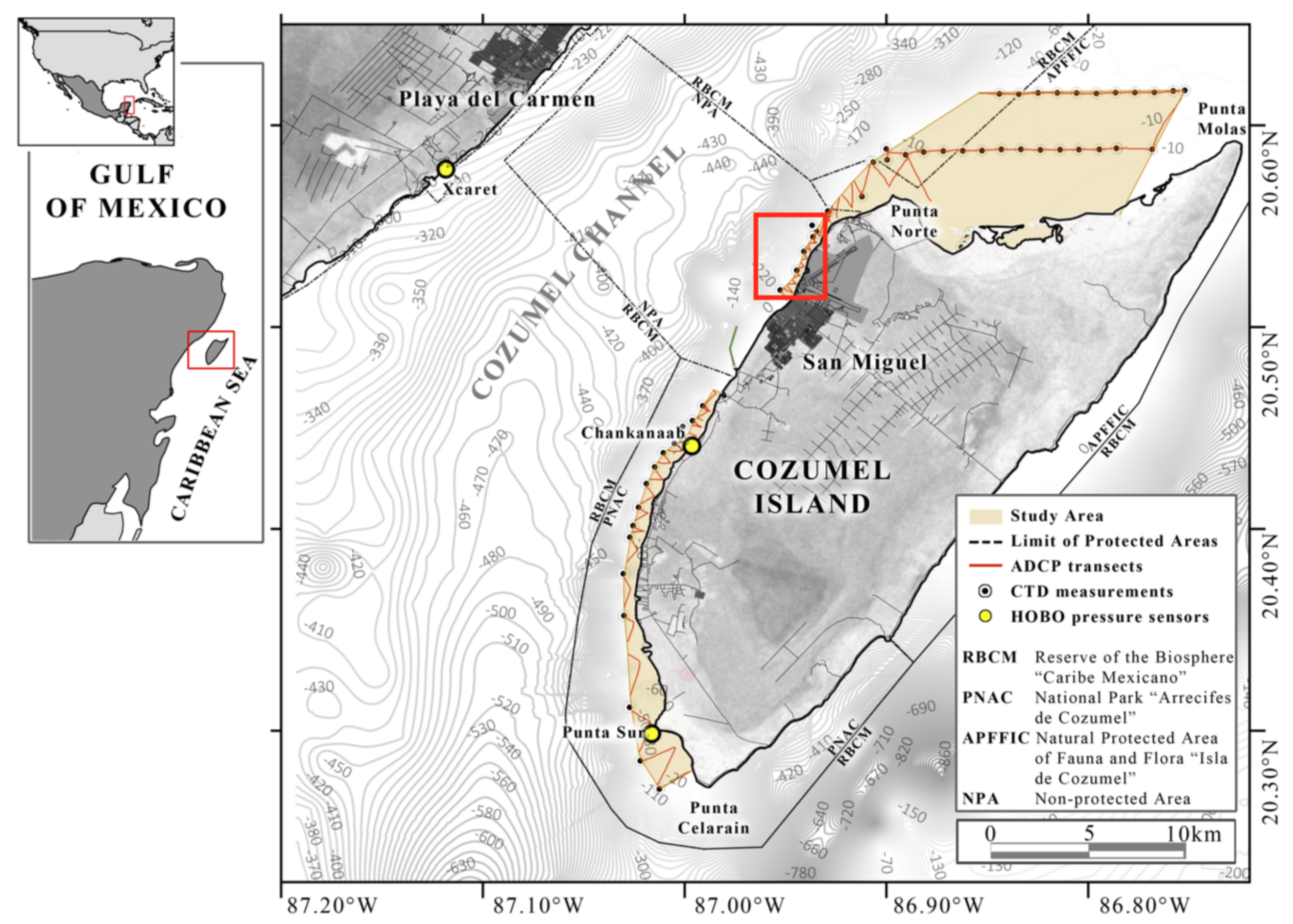
2.2. Potential of Ocean Currents

The shelf around Cozumel Island, Mexico is shown in Figure 3, where the sea is 35–50 m deep at 250–500 m from the coast, and has a fluid density of 1023.6 kg/m 3 [6].
Ocean currents in the Cozumel Channel are promising for generating electric power. According to the reported data, the annual average velocity of the ocean currents in the research area is between 1 and 1.2 m/s, with an increase of 0.05 to 0.06 m/s per kilometer [6] towards the center of the channel. From (1), the marine power, P o , arriving at the turbine, with an annual average fluid velocity of 1.1 m/s and a turbine diameter of 21 m (typical commercial marine turbines), becomes:
P o = 1 2 × 1023.6 × π × 21 2 2 × 1 . 1 3 = 235.94 kW
When a turbine with C p = 0.4 receives 235.94 kW from marine currents, the output power is rated 235.94 kW × 0.4 = 94.376 kW. The turbine could generate 94.376 kW × 365 × 8 = 275.557 MWh if it ran for an average of 8 h per day, throughout the year (a plant factor of 33%), ignoring conversion losses and net speed changes.
A turbine diameter of 21 m was chosen since this is the typical size of a commercial turbine. For example, the Andritz Hydro® HS1000 and HS300 turbines have a 21 m diameter, three-blade horizontal axis rotor, and can generate up to 1 MW at a voltage of 7.6 kV from sea current speeds of 1.0 m/s at a depth of 35–100 m [38]. According to Bárcenas Graniel et al. [7], a SeaGen double marine turbine with an 18 m diameter can generate 380 MWh per year.

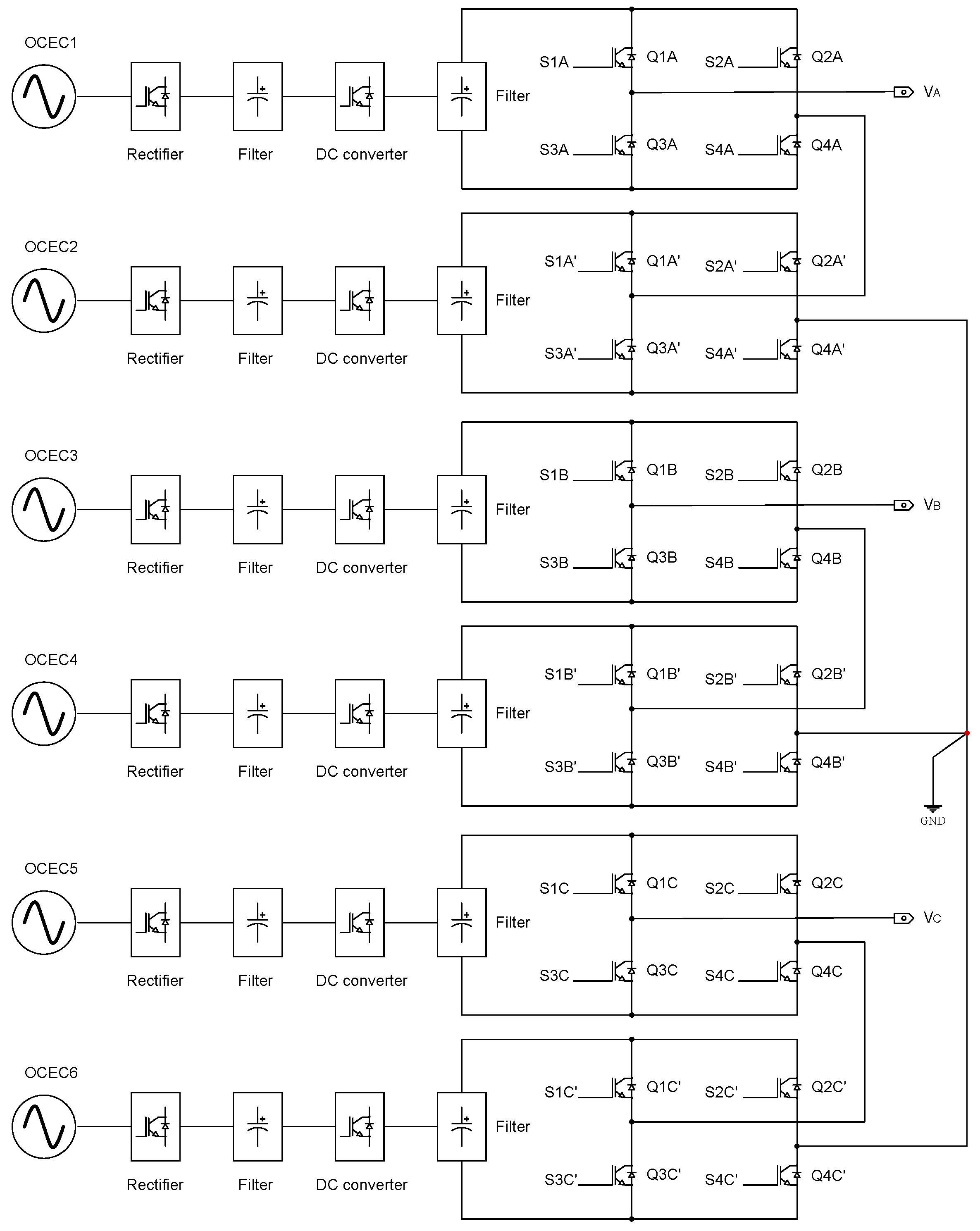
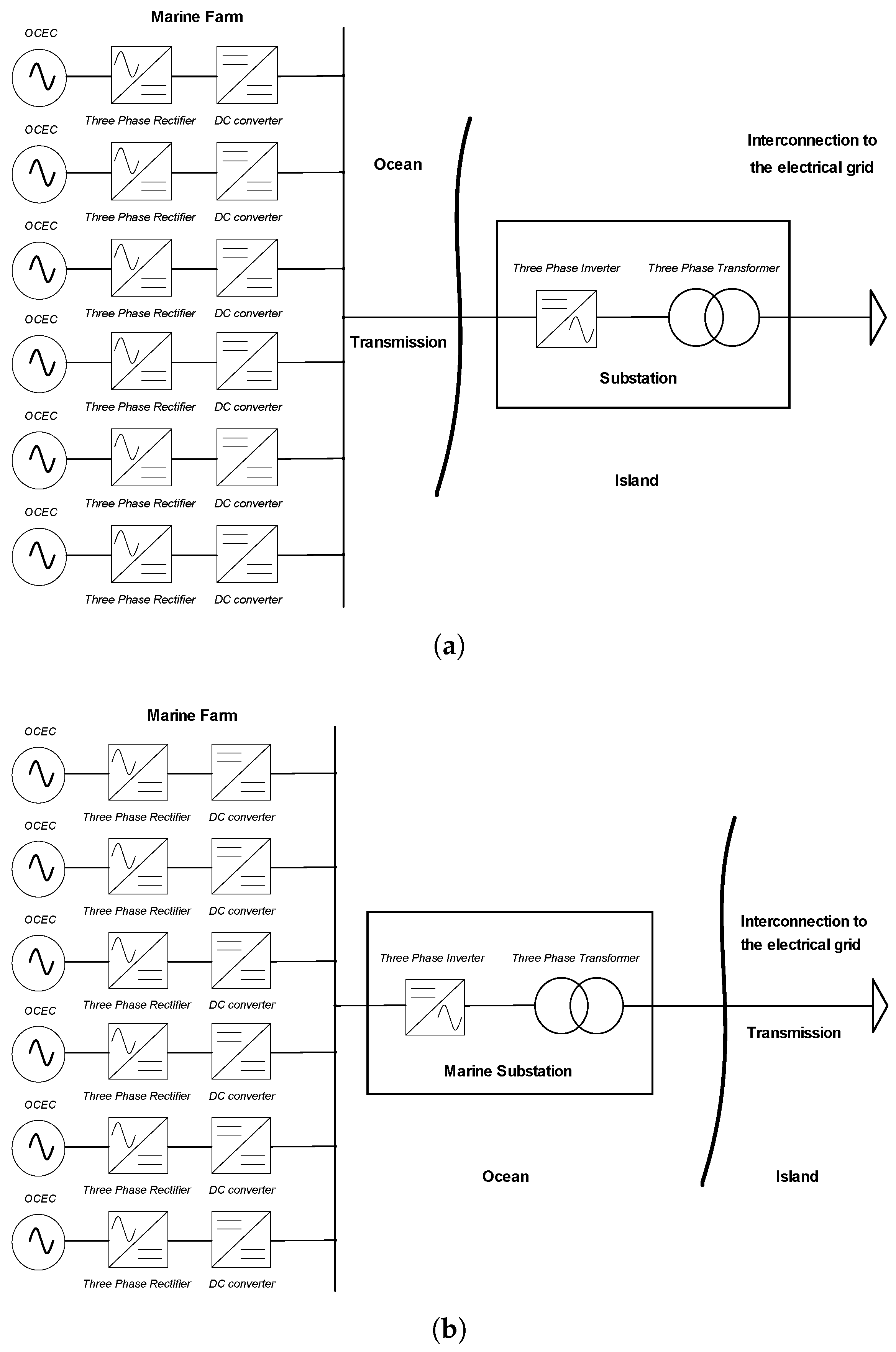
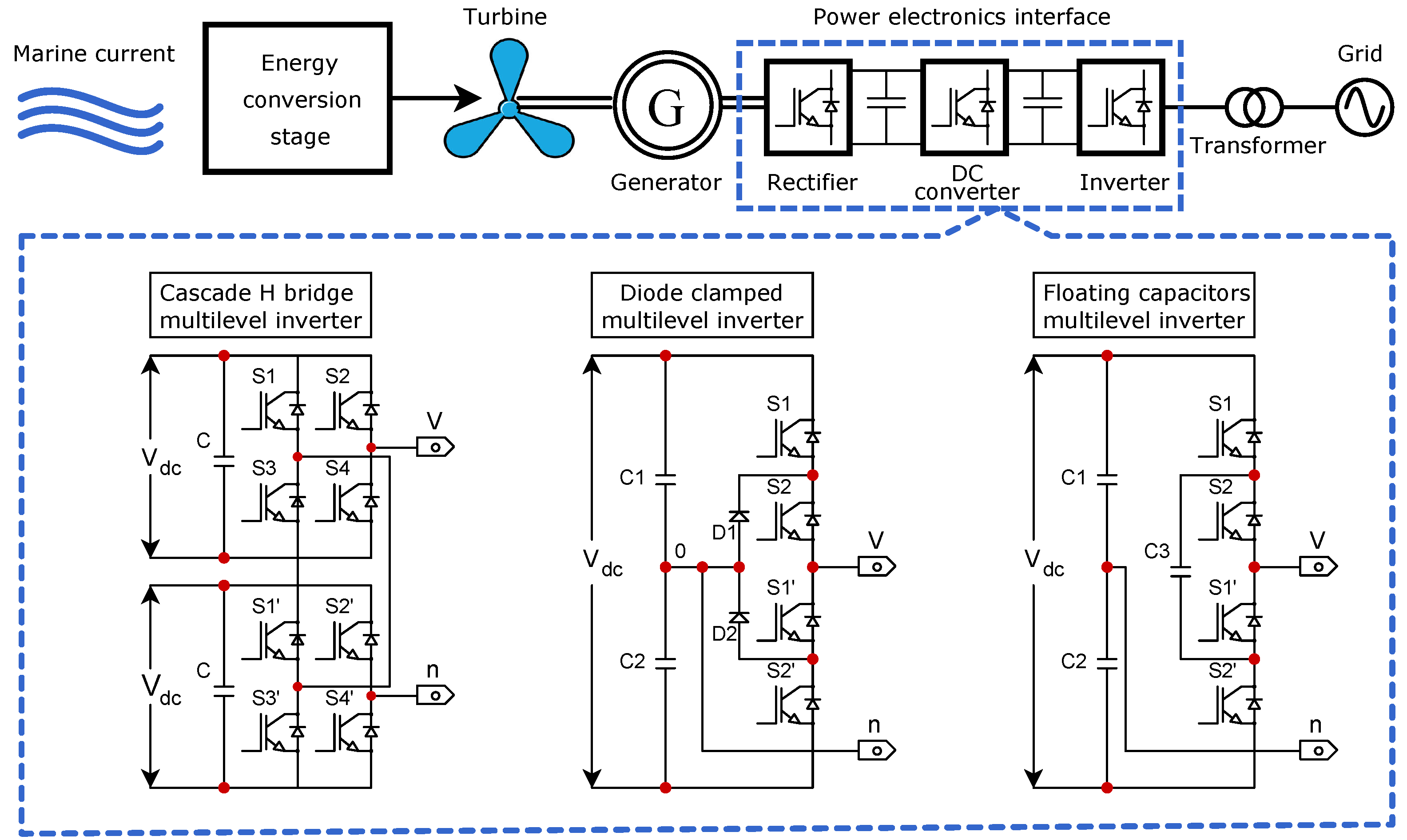
2.3. Electrical Connection and Interconnections

In general, all alternating electric systems require energy conditioning through a power converter for connection to a power grid, with the inverter playing a key role. The power converter should be designed and arranged in such a way that it allows the system to run efficiently and ensures maximum continuity, regardless of faults in the system or disruptions to it [11,12].
Depending on the particular application, multilevel power inverters in renewable energy systems have diverse topologies [39]. The benefits of the multilayer structure come from their ability to lower the harmonic content of the output voltage produced by adding a zero voltage level [13]. Depending on the topology used, the number of multilevels can be increased by adding switching and other passive devices [40].
The full H-bridge multilevel inverter (HBMLI) is a power inverter that can work with independent sources without the use of diodes or capacitors to clamp the voltage. The technique has less sophisticated switching device control and a simpler duality design than other inverter designs. The number of levels (m) and modules (k) shown in [15] determine its setting, as indicated in:
m = 2 k + 1
More levels can be achieved with fewer components in the cascade design (CHBMLI or CHBI) that operates in a modular format [13]. Based on the series connection of the DC sources, the device produces a maximum peak output voltage. It also ensures the operation is ongoing in the event of a DC source failure; if additional robustness is needed, modular cascading allows the addition of more inverter units without the need to reconfigure the entire inverter scheme.
Figure 4 shows a 5-level single-phase CHBI used to harness the power generated by two marine turbines in isolation that can resist high operational voltage stress [41]. Between the OCECs and the inverter, a PWM rectifier and DC converter are considered.
PWM rectifiers reduce harmonic pollution, maintain a power factor, regulate the DC bus voltage, and work with a variable frequency from the generator; the latter is important because the variability of marine currents and the load connected cause a significant change in the frequency of the waveform [42,43,44]. After the PWM rectifier, the DC converter delivers a different voltage level than the DC link, but a voltage gain of over five times the input (or a similarly sized reduction, if it works as a buck converter) is not allowed.
This converter is very popular in renewable energy applications because it supplies a constant voltage input to the inverters and can modify the duty cycle according to system requirements (in this case, it can reduce the level of OCEC voltage according to the nominal parameters of the prototype) [45,46].
Power quality is optimized to meet international requirements as filters are added at the output (not considered in the previous scheme) and multilevel control mechanisms. To replicate the results achieved in this study in three-phase systems, a 120 voltage phase wave shift is required, and the system must be balanced.
Figure 5 shows an example of a six turbine farm, connected to integrate a three-phase inverter cascaded by 5-level H-bridges. This design of this arrangement was based on the analysis of the study inverter configuration and the operation of the OCECs [41].
Continuing with the example of Section 2.1, where a developed power of 94.37 kW per turbine and OCEC was estimated, and applying the scheme of Figure 4, a total of 94.376 kW × 2 = 188.752 kW would be available per phase. If the output voltage per turbine is 7 kV, then the voltage per phase would be 14 kV. The commercial value of 7 kV per OCEC was taken from the European Marine Energy Centre (EMEC) [9].
It is possible to maintain a constant DC link voltage suitable for the nominal voltage value of the components in the circuit using the schematic diagram in Figure 4. If the previous power electronics stage cannot give the appropriate voltage level, a suitable combination of series-parallel IGBTs (with voltage division) allows the nominal voltage values presented in this paper to be used, or any other voltage level [47].
With the configuration shown in Figure 5, a three-phase power of 188.752 kW × 3 = 566.256 kW can be generated, with a line-to-line voltage of 14 kV × 3 = 24.24 kV, star connection. To include more OCECs, an arrangement with multiple levels (CHBMLI) can be used to change the values. It is worth noting that the turbines must all be identical. It should be remembered that high switching frequencies generate considerable heat in semiconductor devices [13,48].
Figure 6 shows two arrays that could be used to connect a marine current generation system like that proposed for the Cozumel Channel. According to Rezini et al. [49], a 5-level CHBMLI has a superior cost/benefit ratio than those with more or fewer levels, and is somewhat higher than other configurations. This is due to the fact that the percentage of waveform voltage distortion is quite similar and has similar effects as others, while its construction and control are less complicated [13,50,51].
It is important to note that, as the number of levels increases, modulation control becomes more difficult, and configuring the control is not an easy task [51]. Another key feature of multilevel inverters is that they lower the number of filters or auxiliary compensation systems that are required [13].

3. Prototype Model

3.1. Prototype Specifications

The printed circuit board (PCB) used for the 5-level single-phase CHBI prototype was designed using EasyEDA software (free use). On the copper tracks for the power stage, there were two layers of copper (upper and lower) with a weight of 28.70 g and a width of 6 mm.
The main technical specifications of the prototype are listed in Table 1. The nominal parameters were determined using the maximum supported current value of the PCB tracks [52] and the IGBT voltage [53], as well as the power stage of the connectors and terminals. Considering the greatest switching frequency (2940 Hz) and the test parameters, a 10 μ F/600 V DC link capacitor was used [54].

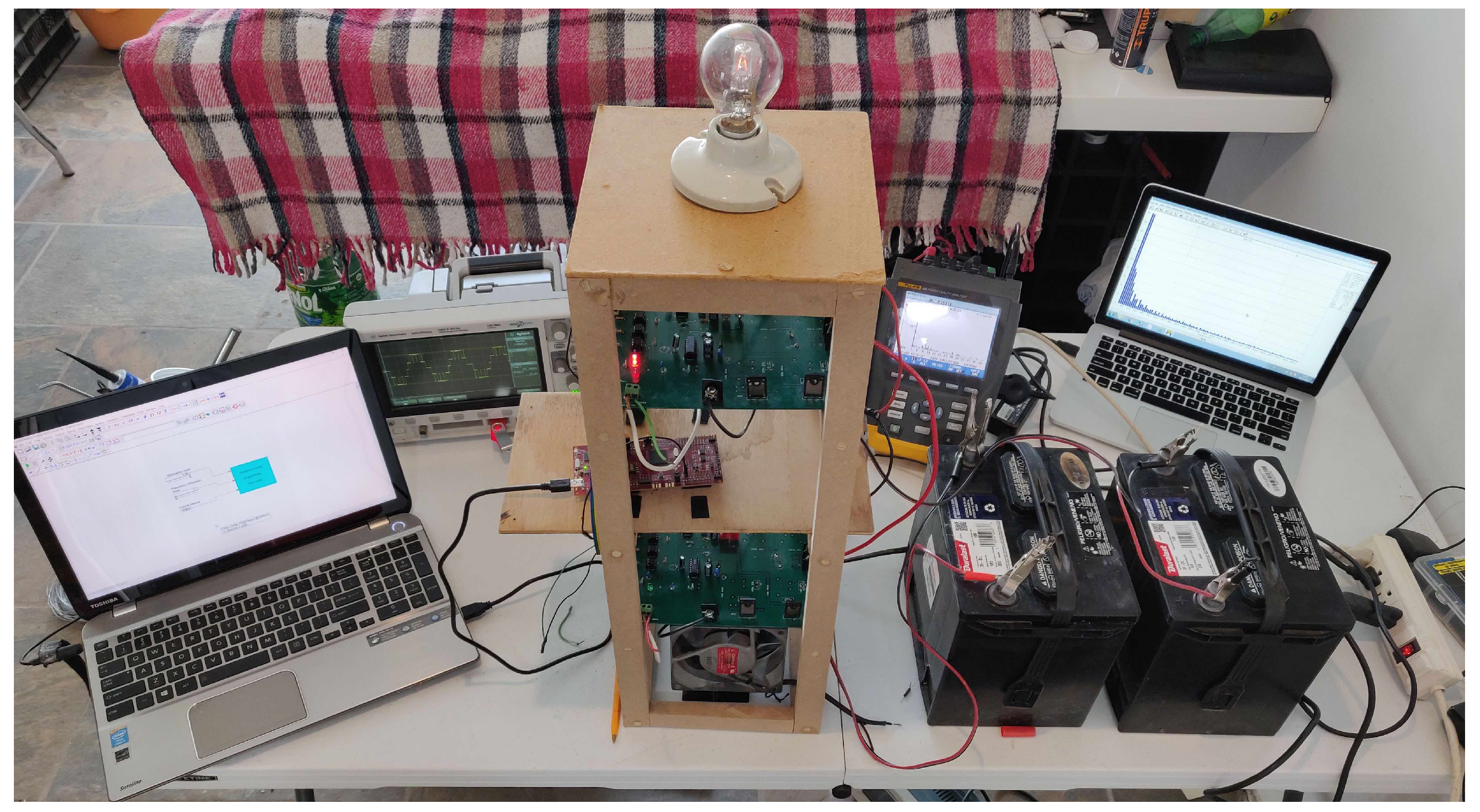
3.2. Equipment and Test Conditions

Due to the limited DC sources available in the laboratory, the inverter tests were not performed with their nominal values; as a result, heat sinks were not required for testing values, although they were considered for future inclusion in the PCB design. As shown in Figure 4, constant DC sources were used assuming an input with little change (standard requirements for interconnection of renewable sources to the grid). The power supply was two DC batteries of 12 V d c y 550 A each. The testing included both resistive and inductive-resistive loads. The prototype inverter and the testing equipment are shown in Figure 7.

4. Control Methods Applied

The LS-SPWM control methods used to generate the trigger signals of the 2 k + 1 level with k = 2 were obtained by applying a reference signal (sine wave) and a high frequency carrier signal (triangular wave). Comparison of both signals produced the two states (high or low).
Only the odd components were addressed in the design of the LS-PWM control, which used carrier waves ranging from 660 to 2940 Hz (11th to 49th component, respectively). The modulating wave had a frequency of 60 Hz.
The frequency of the carrier signal was the switching frequency of the inverter. The reference (modulating) signal is described as:
h V m , f m , t = V m sin 2 π f m t
where h is the sine wave, V m is the peak amplitude of the modulating signal (V), f m is the frequency of the modulating signal (Hz), and t is the time (s).
The number of carriers n c required for control is given by
n c = m 1
The n c carrier signals used were obtained with
g V c , f c , ϕ c , n c , k , t = 2 V c f c 1 2 f c t + ϕ c mod 1 f c 1 2 f c + n c k k
where g is the trigger signal, V c is the peak amplitude of the carrier signal (V), f c is the frequency of the carrier signal (Hz), and ϕ c is the phase angle.
The high and low states for levels i < k + 1 , where i = 1 , 2 , , k , were calculated
g V c , f c , ϕ c , i 1 , k , t > h V m , f m , t
Similarly, the levels i > k + 1 , where i = k + 2 , k + 3 , , 2 k + 1 , were calculated
g V c , f c , ϕ c , i 2 , k , t < h V m , f m , t
In multilevel inverters, multicarrier waveform modulation is controlled by the amplitude and frequency modulation indices [13,41,55], given by (9) and (10).
m a = V m V c ( m 1 )
m f = f c f m
The representative control diagram for the LS-PWM control is shown in Figure 8, with the carriers ordered from top to bottom. According to the LS-PWM modulation, each carrier signal is displaced on a separate level of DC, with the amplitude of each modulation scheme defined by the m a used. In all the tests, a constant value of amplitude modulation was used m a = 0.99 , as this value was identified to produce lower harmonic component magnitudes. In this study, the analysis of phase shift and the frequency for each carrier signal with each control scheme was important. The control methods applied to the prototype inverter are shown in the following sections.

4.1. In-Phase Disposition (IPD) Control

In this method of control, all the carriers are in phase ( ϕ c = 0 ) for the creation of the trigger control signals [13,14,15]. Furthermore, all the carriers above and below zero have the same frequency, amplitude, and phase, but a distinct DC offset (Figure 9).

4.2. Alternate-Phase Opposition–Disposition (APOD) Control

The odd levels i < k + 1 and i > k + 1 in this control method are out of phase ϕ c = 180 from their adjacent or alternating carrier with ϕ c = 0 [13,14,15] (Figure 10).

4.3. Phase Opposition–Disposition (POD) Control

In this arrangement, all the carriers with a value greater than zero (levels i < k + 1 ) have the same phase ϕ c = 0 , whereas carriers below the zero reference (levels i > k + 1 ) are in phase with each other, and ϕ c = 180 is out of phase with those above the references [13,14,15] (Figure 11).

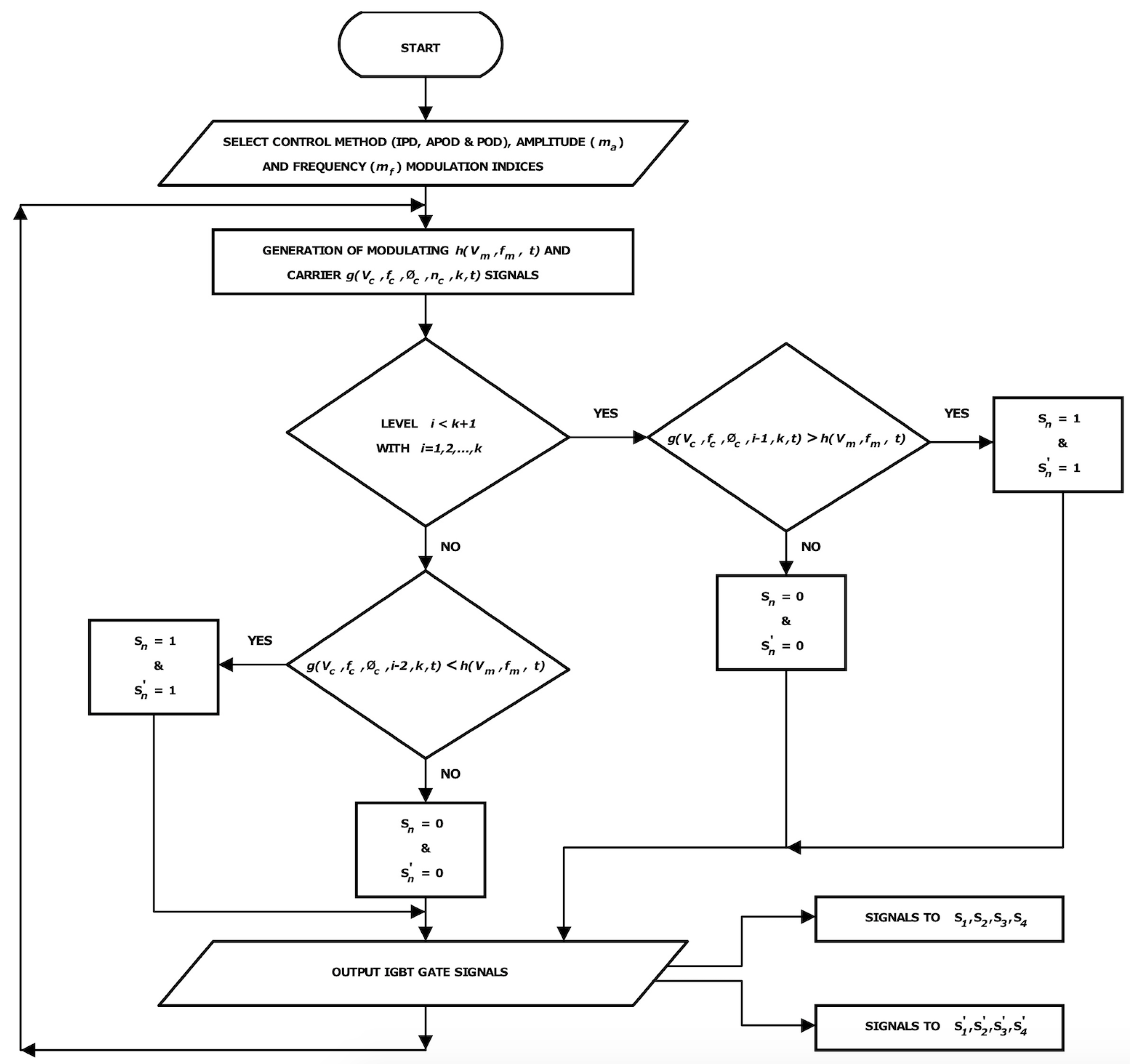
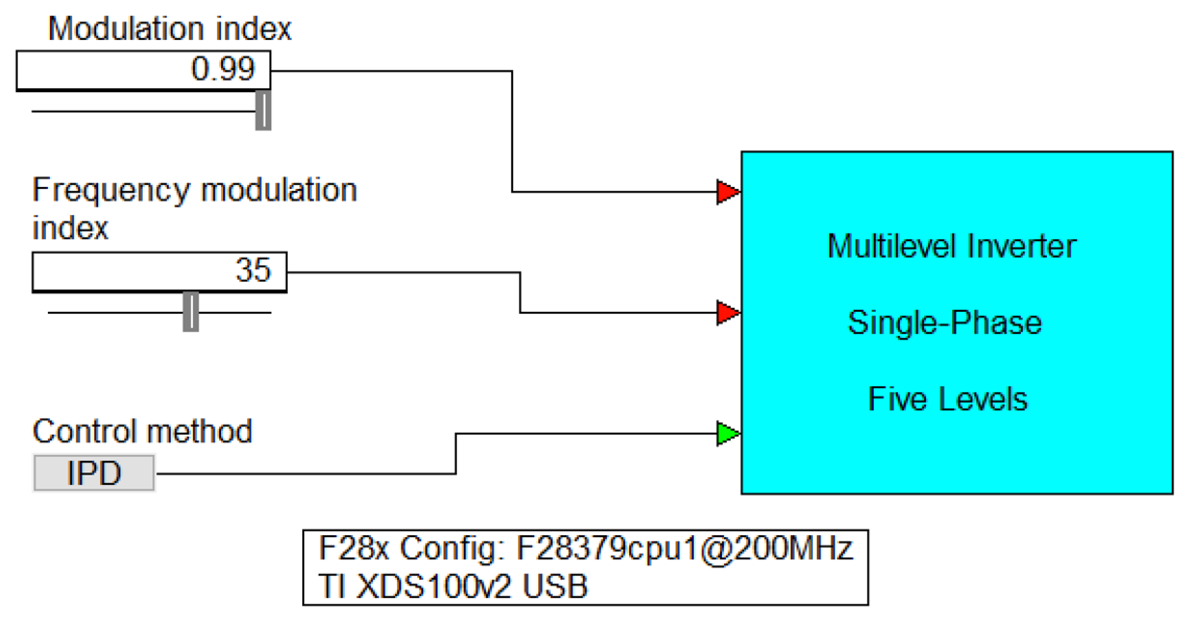
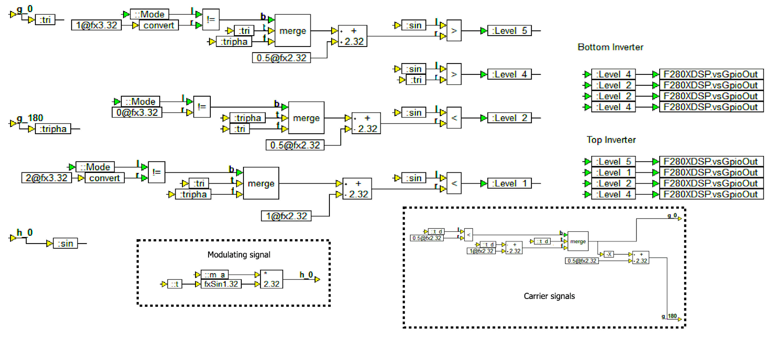
5. Implementation of the Control Program

The inverter was controlled using a Texas Instruments® microcontroller TMS320F28379D and a 2019 student edition of SolidThinking Embed® software, which allows for the selection of m f , m a , and IPD, APOD, and POD controls. A flowchart of the proposed LS-PWM control algorithm is shown in Figure 12. The embedded scheme of the program is seen in Figure 13, and Figure 14 gives the block scheme of the control algorithm. This program uses fixed point type blocks for the variables.

6. Analysis of Results

For each method of control, the results were analyzed focusing on the voltage waveform, harmonic content, and voltage THD. The load current waveform distortion was observed but was not evaluated for the purpose of this paper.
A first analysis was performed using the IPD method, applying resistive load, with m f = 11 and m a = 0.99 values. Then, for comparison, the modulation index m f was varied applying the values of 19, 29, 39, and 49, to identify the variations in the waveform, harmonic content, and THD.
For a second analysis, an inductive-resistive load of ratio X L / R = 3.06 was applied, using the same modulation indices as in the first analysis. The procedure was repeated for each control method.
It is assumed that the response of the single-phase prototype would be quite similar to that of a balanced three-phase system, except for the behavior of third order harmonics.

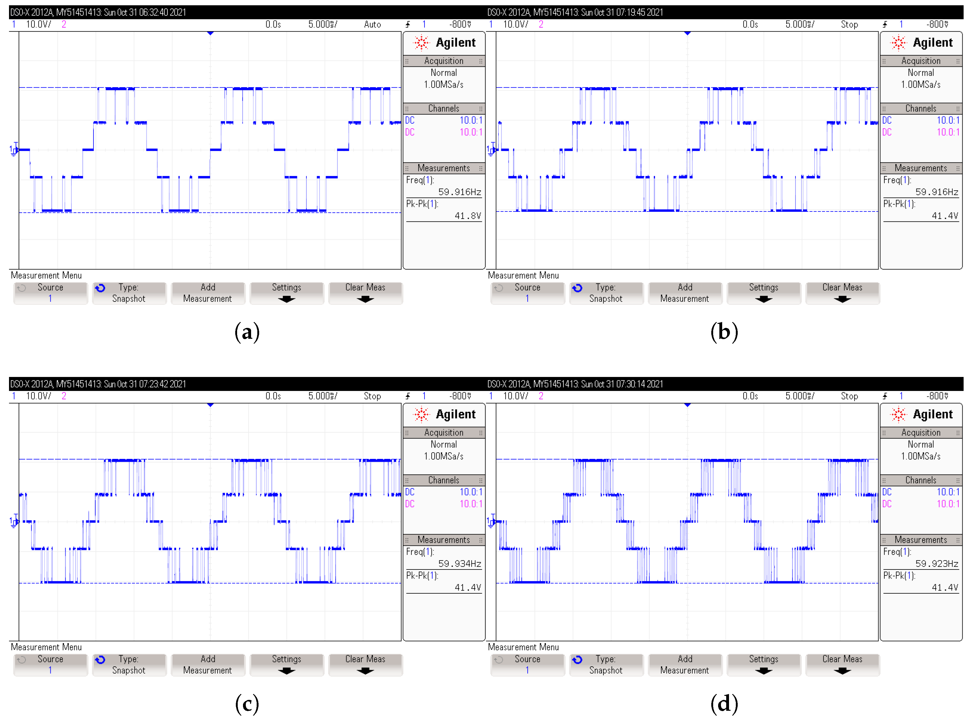
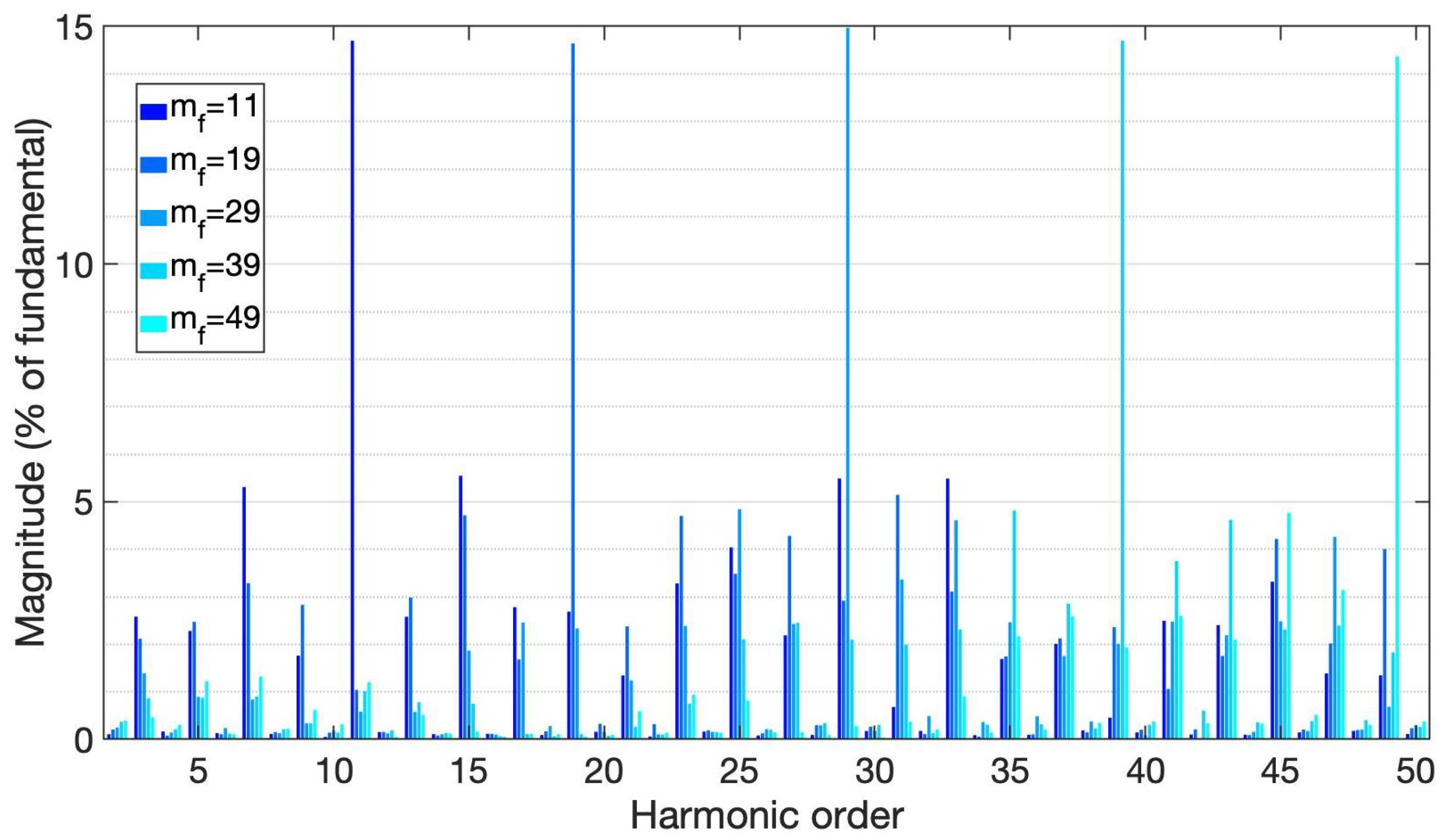
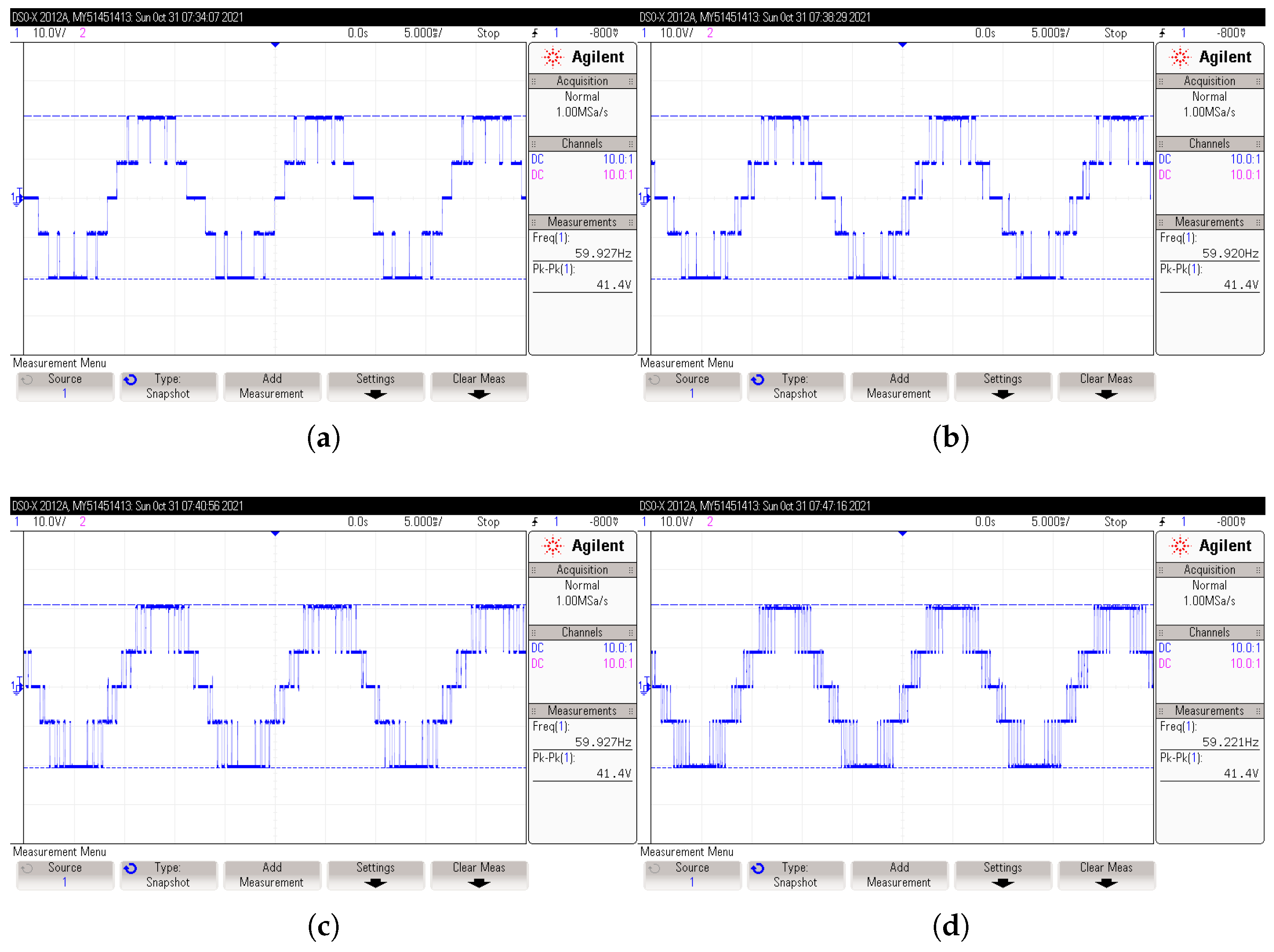
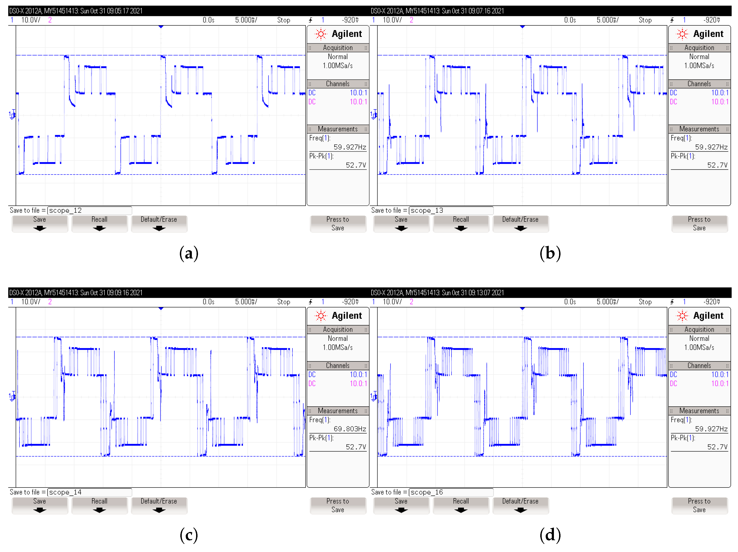
6.1. Results with IPD Control

Figure 15 shows the output voltage performance under resistive load conditions, and Figure 16 shows the harmonic spectrum considering the range of m f values. Note that the first harmonic has been removed from the plots to give better detail of the remaining components.
It can be seen that, when m f increased, the voltage waveform was more robust, and the odd harmonics of increasing magnitude moved closer to the high frequency. The waveform frequency was from 59.916 to 59.923 Hz.
With the IPD control method, there was a relatively low harmonic content under resistive load, with the smallest components below 5% of the fundamental. The highest magnitude reached almost 15% (note the displacement that this component undergoes when m f varies, locating itself in the values of m f used). The largest component decreased as m f rose.
Compared with the results of the simulations of the IPD control and other PWM methods presented in [30,31,32,33,34,35,36,37], under resistive load, there is a similarity in the output voltage waveform and the harmonic spectrum. There is also a considerable reduction in the magnitude of the highest component under any m f .
Figure 17 and Figure 18 show the output voltage and the harmonic spectrum, obtained under inductive-resistive load, respectively.
In contrast to the voltage waveform obtained under resistive load, the waveform obtained under inductive-resistive load showed an abrupt distortion and an increase in magnitude (approximately 12.1 V). The zero voltage level had a level-shift higher than the positive and negative peak values. As m f increased, the waveform became more robust and the distortion behaved in a similar manner.
The frequency did not vary much when compared to the results with resistive load (59.920 to 59.927 Hz).
Under inductive-resistive load, the harmonic content increased dramatically. There are three degrees of significance: first, the components of greater magnitude that are close to 25%; second, the components with an average value near 10%; and, finally, the components of smaller magnitude, below 5%.
The largest components (660 and 1140 Hz) were produced with m f values of 11 and 19. It is clear that the 3rd component did not vary significantly as the m f varied, but there was no noticeable difference between the 5th and 15th components when applying m f values of 29, 39, and 49.
As in the previous analysis, there were no even components and DC presence of significant value.

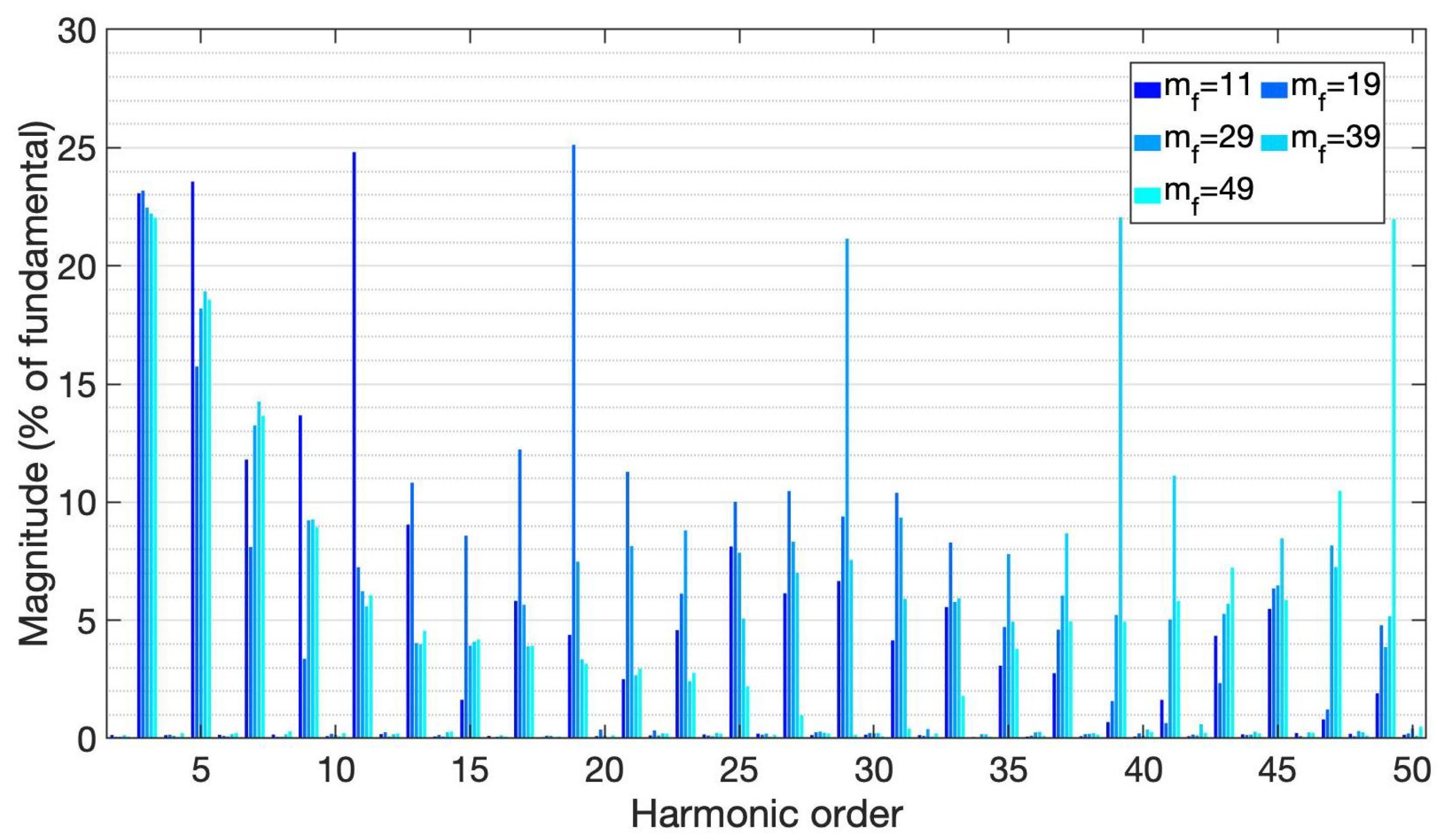
6.2. Results with APOD Control

Figure 19 shows the voltage behavior under resistive load with different m f values. In comparison to the IPD approach, it is seen that the pulse width changes in the lower lobes of the voltage waveform.
Figure 20 shows the harmonic spectrum obtained with the APOD control method. As shown later, this gives a smaller percentage of total harmonic distortion (THD).
The amplitude (41.4 V) and distortion behavior were nearly identical to those obtained in IPD control, while the frequency changes were from 59.221 to 59.927 Hz (0.696 Hz less than the range in IPD method).
As the components approached high frequency, their behavior was fairly similar. Unlike the prior control method, the component with the highest magnitude was not located in the m f used. It can be seen that, unlike the IPD control method, the even harmonic components had the greatest magnitude (close to 10%), although they were not as large as those given by the harmonic content of the IPD control method. Using a m f of 49, the fundamental component was almost 88%, but dropped to 85% when using a m f of 11; when compared to earlier results using the IPD method with resistive load, the percentage of the fundamental component was smaller.
It is interesting to note that the harmonic component with the greatest amplitude was five orders behind the m f applied. When the m f was 11 and 19, the largest components were created (660 and 1140 Hz).
Comparing the APOD control and other PWM modulation results with the simulations reported in [30,31,32,33,34,35,36,37], under resistive load, the output voltage waveform is similar, and there is a considerable reduction of the highest magnitude component in the harmonic spectrum.
Figure 21 shows the output voltage behavior, and Figure 22 shows the harmonic spectrum obtained with the APOD control, under inductive-resistive load.
Under inductive-resistive load, the voltage waveform had a small distortion at the peaks, due to the zero level shift when compared to the harmonic content results of the IPD control method, but the magnitude was greater (0.8 V larger). The frequency did not differ much from the values obtained in the IPD approach, but, with m f = 29 , the frequency increased to 69.813 Hz.
The harmonic content behaved similarly to the previous control method, with the exception that the components of greater magnitude were close to 18%, while those smaller in size were below 5%. However, it is clear that there are even components of considerable magnitude in this method; the 3rd and 5th components were the most significant (180 and 300 Hz). From the 3rd to the 11th odd component, the behavior was fairly similar to the IPD control technique. When m f = 11 was used, there was a substantial DC component (nearly 1%).

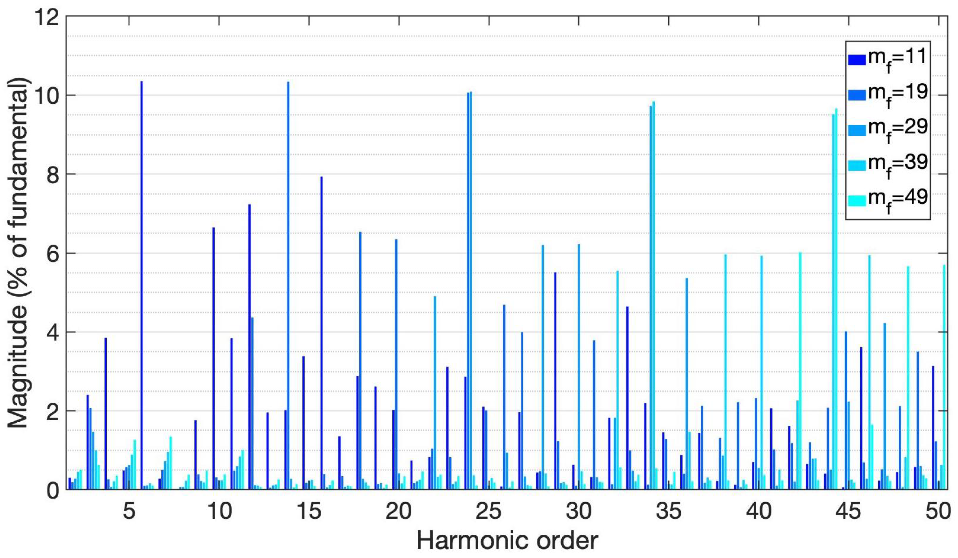
6.3. Results with POD Control

Because the POD and APOD methods use identical modulation criteria, the results achieved with the POD approach are similar to those obtained with the APOD method. The distortion of the signal was quite close to that produced using the IPD approach. Figure 23 shows the voltage behavior under resistive load conditions with various m f values. Figure 24 shows the harmonic spectrum with a POD control approach.
The POD method had different amplitude and frequency values than the IPD and APOD methods, but the waveform peaks followed the same pattern as the preceding ones. In both IPD and APOD, the variation in frequency was greater. The lowest and highest deviations with the prior approaches were 0.066 and 0.073 Hz, respectively, over the 60 Hz fundamental, while the lowest and highest deviations with POD were 0.073 and 2.158 Hz, respectively.
In comparison to the waveforms in Figure 15 and Figure 19, the voltage amplitude was reduced by 0.8 V. The waveform was almost identical to the previous control techniques due to the robustness created by increasing the m f to 49. However, examining the harmonic spectrum and THD, it was found that the harmonic content was very different—higher in some approaches than others. It is interesting to note that the harmonic component with the highest amplitude was one order behind the m f used. When employing a m f of 11 or 19, the highest components were created (660 and 1140 Hz).
Compared with the simulation results of the POD control and other PWM methods reported in [30,31,32,33,34,35,36,37], under resistive load, the output voltage waveform and harmonic spectrum are very similar. In most cases, there is a considerable reduction in the magnitude of the highest harmonic component.
Figure 25 shows the output voltage behavior, whereas Figure 26 shows the harmonic spectrum applying the POD control method, under an inductive-resistive load.
When comparing the harmonic content from the IPD and APOD control methods with inductive-resistive load, the voltage waveform had the same magnitude and distortion in the peaks as the APOD approach, but not as the IPD method.
The frequency variation was almost identical to the results obtained using the IPD and APOD methods with an inductive-resistive load; however, when m f = 29 was used, the frequency increased to 69.803 Hz.
The harmonic content was similar in behavior to that of the prior control method, except that the components of greater magnitude were below 18% and the smaller ones were below 5%. There are even components of significant magnitude in this method, where the 3rd and 5th components were the most significant (180 and 300 Hz). The amplitude of the odd components from the 3rd to 15th was very similar regardless of the m f applied. It was also very similar to that of the APOD control, and very different from that of the IPD.

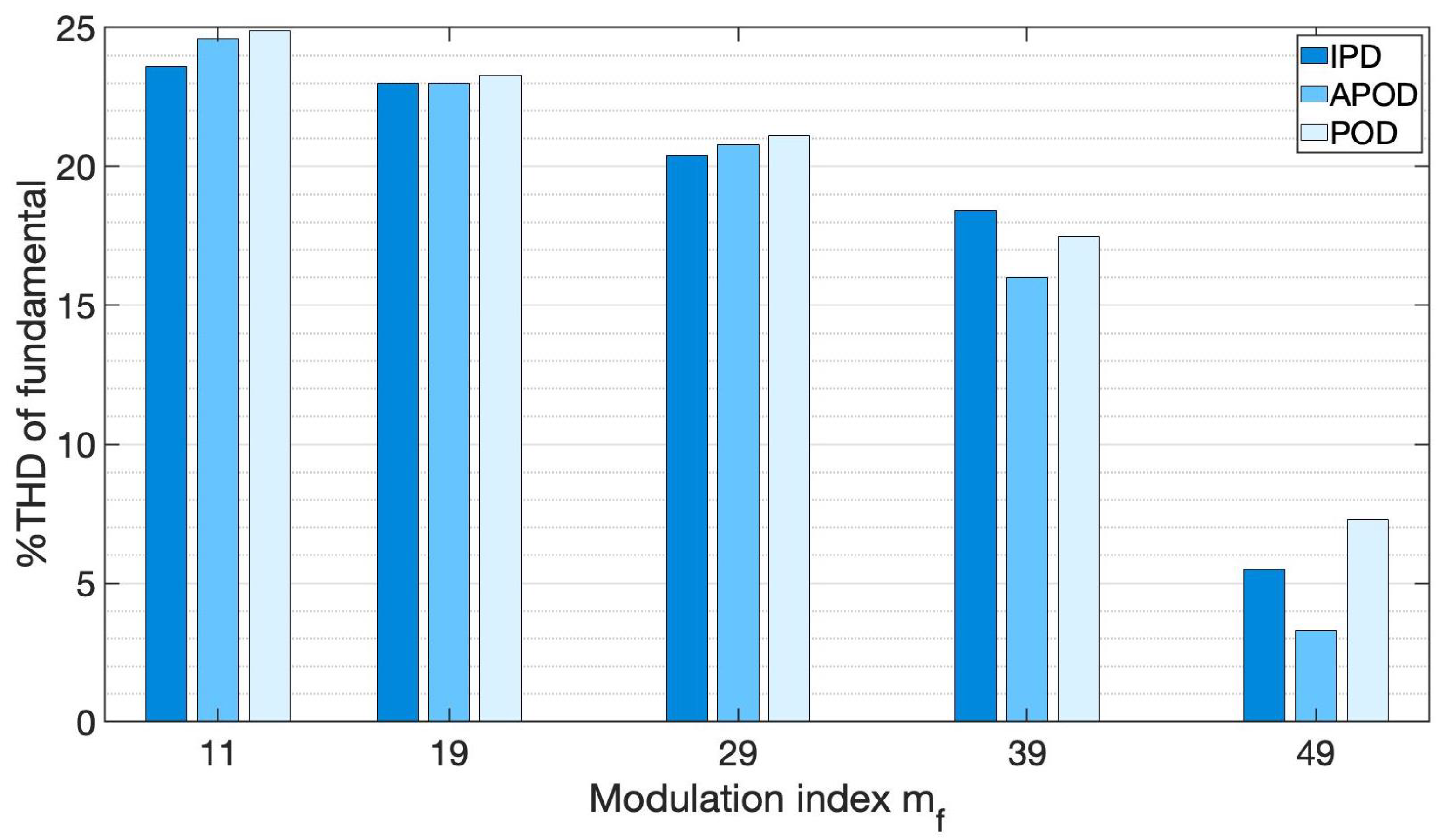
6.4. THD Results with Resistive Load

Figure 27 shows the THD of the 5-level CHBI output voltage, applying the three distinct control methods under resistive load for each m f considered.
When m f = 11 was used in IPD control, the overall THD was 23.6%. However, when the m f was increased to 49, the total THD was 5.5%. A direct examination of the harmonic components is possible with a resistive load, and it is clear that this is directly dependent on the m f value. The harmonic components were significantly reduced with high m f values.
At m f = 11 , applying the APOD control, a THD of 24.6% was obtained. The overall THD fell to 3.3%t when the m f was increased to 49. However, when m f = 11 , the THD was 1% greater than when using the IPD control. Because lower frequency harmonic components were practically inconsequential, and the measurement instrument did not consider components beyond the fifteenth harmonic, this THD was the lowest of the three methods for high m f values. In this method, the even harmonic components had the highest magnitudes.
With the POD method, a THD of 24.9% was obtained with a value of m f = 11 . If m f = 49 , the total THD fell to 7.3%. Note that, in this method, the even harmonic components had the highest magnitudes. However, THD was higher than that in previous cases when m f = 49 ; 4% higher than the APOD method and 1.8% higher than the IPD method. It was thus evident that, in all three methods of analysis, the THD decreased as the value of m f increased.
A THD of 24.9% was obtained using the POD control, with m f = 11 . The overall THD fell to 7.3% when m f = 49 . The even harmonic components had the highest magnitudes in this control. However, using m f = 49 , there was a greater THD than in earlier situations; 4% higher than the APOD approach and 1.8% higher than the IPD method. In the three control methods, the THD decreased as the value of m f increased.
When compared to the POD technique, the APOD method gave a lower THD for all m f values. However, when the m f was 11 and 29, the THD percentage was larger than the IPD control.
A reduction in the THD level under resistive load was obtained compared to the results presented in the previously cited references, where the LS-PWM method and other modulation techniques, such as space-vectors or selective harmonic elimination techniques for 5-level inverters, were employed.

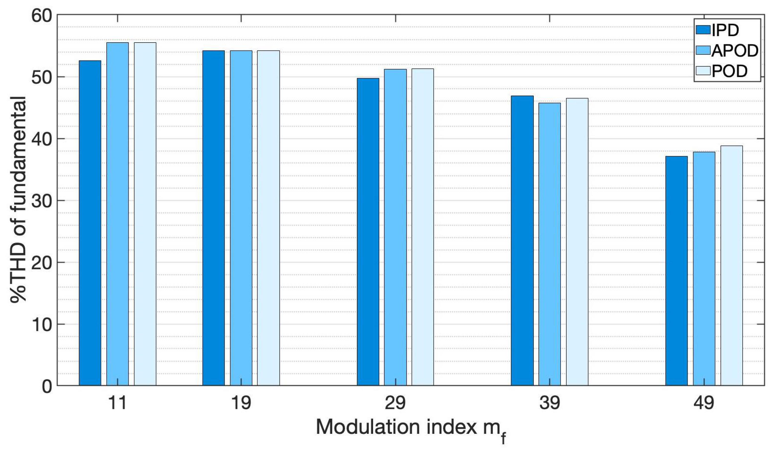
6.5. THD Results with Inductive-Resistive Load

Finally, Figure 28 shows the THD for each m f considered, applying the three control methods with inductive-resistive load.
The direct examination of the harmonic components produced for each control approach was more complex; increasing the m f did not ensure a reduction in THD as occurred as in the previous instances. In IPD control, m f = 11 had a THD of 52.6%; however, when the m f was increased to 49, the total THD dropped to 37.1%.
At m f = 11 using the APOD control, a THD of 55.5% was obtained. However, increasing the m f to 49 reduced the overall THD to 37.8%. With m f = 11 , the THD was 2.9% greater than with the IPD approach.
The POD technique had a THD of 55.5% with a value of m f = 11 . When m f = 49 , the total THD dropped to 38.8%. With m f = 49 , however, a higher THD was given than in the preceding situations; 1% higher than the APOD approach and 1.7% higher than the IPD method.
The IPD approach had a smaller THD than the other methods when using m f values of 11, 29, and 49. Using m f = 39 , the THD values when using the APOD technique were only slightly lower than in the preceding case.
It is important to mention that this THD analysis approach for a multilevel inverter, under different types of load, has not been studied in great depth as yet.

7. Discussion and Conclusions

The inverter with a resistive load showed acceptable tolerance in the voltage waveform, harmonic content, and voltage THD. The results were better than those presented by Solangi [56] and similar to configurations of seven or more levels reported by Rezini et al. [49] and Soomro et al. [57]. This feature is deemed vital for its usage in OCECs due to its modular operation. It also offers better efficiency in this application than photovoltaic systems. Under a resistive load, the results of the frequency fluctuations show acceptable behavior, with a deviation that is within the tolerance range allowed in Mexican regulations [29].
The waveform deformation caused by the presence of a large number of harmonics of significant amplitude is seen in the findings obtained using an inductive-resistive load. The frequency variations, on the other hand, are low, due to careful selection of the control technique and the m f value (with values of 29 and 39, there were very high deviations).
Many of the larger harmonic components are easily detected with this sort of analysis, making filter selection easier for improved electrical grid connectivity. For marine turbine configurations in Mexico, the Grid Code reduces its constraints for THD and individual harmonic distortion (IHD) values, assuming operating voltages and capacities below those specified in Section 2.3. For voltage, a THD value of less than 5% is necessary, and for individual components, a THD value of less than 6.5% is required. According to these results, some values are close to those that are permitted under resistive load (the use of filters is mandatory in connectivity). However, with an inductive-resistive load, a high m f may be used to shift the components with larger amplitude towards the high frequency and eliminate them using low-pass filters. This was done with the understanding that, as the magnitudes of the high frequency components decrease, the price of the filters decreases (as shown in the analyses performed under various loads). When selecting filters, this has the advantage that the size of the filters is drastically reduced.
The results obtained in this work show an improved output voltage waveform and a reduction in the THD values, under the resistive and inductive-resistive load values considered when compared with those of [17,18,19,30,31,32,33,34,35,36,37,56,58], where other inverter topologies and PWM modulation methods were analyzed. It can be said that the implementation of the control scheme and the topology applied to the prototype are suitable for developing a practical three-phase inverter model.
The research described in this paper is based on a laboratory prototype. Using the theory and analysis presented, it is feasible to investigate offshore ocean current power interconnection applications, where findings may be compared (potential for Cozumel, arrangement and control methods applied). In conclusion, the findings from the single-phase prototype suggest that three-phase systems might benefit from the results found in this research.

Author Contributions

Conceptualization, L.A.G.-R., A.B.-T. and F.B.-R.; methodology, L.A.G.-R., A.B.-T., F.B.-R. and M.R.-H.; software, L.A.G.-R. and A.B.-T.; validation, L.A.G.-R., A.B.-T., F.B.-R., M.R.-H. and J.M.R.-A.; formal analysis, L.A.G.-R., A.B.-T., M.R.-H. and J.M.R.-A.; investigation, L.A.G.-R. and A.B.-T.; resources, L.A.G.-R., A.B.-T. and R.S.-C.; data curation, L.A.G.-R., A.B.-T. and M.R.-H.; writing—original draft preparation, L.A.G.-R., A.B.-T. and M.R.-H.; writing—review and editing, all; visualization, L.A.G.-R., A.B.-T., M.R.-H., J.M.R.-A. and R.S.-C.; supervision, all; project administration, L.A.G.-R., A.B.-T., M.R.-H. and R.S.-C.; funding acquisition, L.A.G.-R., F.B.-R. and R.S.-C. All authors have read and agreed to the published version of the manuscript.

Funding

This work was supported by CONACYT-SENER-Sustentabilidad Energética, under grant FSE-2014-06-249795 “Centro Mexicano de Innovación en Energía del Océano (CEMIE-Océano)”.

Institutional Review Board Statement

Not applicable.

Informed Consent Statement

Not applicable.

Data Availability Statement

The data that support the results of this study are available from the corresponding authors upon reasonable request.

Acknowledgments

This work was supported in part by the Consejo Nacional de Ciencia y Tecnología (CONACYT) under grant FSE-2014-06-249795, and in part by the Universidad Autónoma de Zacatecas (UAZ).

Conflicts of Interest

The authors declare no conflict of interest.

References

  1. Worldometers. Current World Population. Available online: https://www.worldometers.info/world-population/ (accessed on 11 January 2022).
  2. REN21. Renewables 2020 Global Status Report. Available online: https://www.ren21.net/wp-content/uploads/2019/05/GSR2021_Full_Report.pdf (accessed on 10 January 2022).
  3. Tsao, C.C.; Feng, A.H.; Hsieh, C.; Fan, K.H. Marine current power with cross-stream active mooring: Part I. Renew. Energy 2017, 109, 144–154. [Google Scholar] [CrossRef]
  4. Aprendeconenergia. Aprovechamiento de la Energía Marina en el Mundo. Available online: https://www.aprendeconenergia.cl/aprovechamiento-de-la-energia-del-mar-en-el-mundo/ (accessed on 21 January 2022).
  5. Bai, G.; Li, W.; Chang, H.; Li, G. The effect of tidal current directions on the optimal design and hydrodynamic performance of a three-turbine system. Renew. Energy 2016, 94, 48–54. [Google Scholar] [CrossRef]
  6. Alcérreca-Huerta, J.C.; Encarnacion, J.I.; Ordoñez-Sánchez, S.; Callejas-Jiménez, M.; Gallegos Diez Barroso, G.; Allmark, M.; Mariño-Tapia, I.; Silva Casarín, R.; O’Doherty, T.; Johnstone, C.; et al. Energy yield assessment from ocean currents in the insular shelf of Cozumel Island. J. Mar. Sci. Eng. 2019, 7, 147. [Google Scholar] [CrossRef] [Green Version]
  7. Bárcenas Graniel, J.F.; Fontes, J.V.; Garcia, H.F.G.; Silva, R. Assessing hydrokinetic energy in the Mexican Caribbean: A case study in the Cozumel channel. Energies 2021, 14, 4411. [Google Scholar] [CrossRef]
  8. Shirasawa, K.; Tokunaga, K.; Iwashita, H.; Shintake, T. Experimental verification of a floating ocean-current turbine with a single rotor for use in Kuroshio currents. Renew. Energy 2016, 91, 189–195. [Google Scholar] [CrossRef]
  9. EMEC. European Marine Energy Centre (EMEC). Available online: http://www.emec.org.uk/ (accessed on 5 February 2022).
  10. Ropero, I.L. Técnicas de Modulación para Convertidores de Fijación por Diodos tres Niveles Multifase y Control Eficiente de Dispositivos Captadores de Energía de las Olas. Ph.D. Thesis, Universidad del País Vasco, Escuela Técnica Superior de Ingeniería de Bilbao, Biscay, Spain, 2015. [Google Scholar]
  11. Yassin, H.M.; Shafei, M.A.R. Active and Reactive Power Control of Marine Current Turbines with Flywheel Energy Storage System Using Meta-heuristic Technique. In Proceedings of the 2019 21st International Middle East Power Systems Conference (MEPCON), Cairo, Egypt, 17–19 December 2019; pp. 417–422. [Google Scholar]
  12. Pham, H.T.; Bourgeot, J.M.; Benbouzid, M.E.H. Comparative Investigations of Sensor Fault-Tolerant Control Strategies Performance for Marine Current Turbine Applications. IEEE J. Ocean. Eng. 2018, 43, 1024–1036. [Google Scholar] [CrossRef]
  13. Beltrán-Telles, A.; Monteagudo, F.L.; Beltrán-González, C. Energy quality analysis of CH-bridge inverter and SPWM control. Ing. Energ. 2020, 41, 1–11. [Google Scholar]
  14. Shahid, U.; Shafique, A.; Khan, I.; Rahman Kashif, S.A. Implementation of multilevel inverter using space vector pulse width modulation. Sci. Int. 2016, 28, 2451–2455. [Google Scholar]
  15. Maswood, A.I.; Tafti, H.D. Advanced Multilevel Converters and Applications in Grid Integration; Wiley: Chichester, UK, 2018. [Google Scholar]
  16. António-Ferreira, A.; Collados-Rodríguez, C.; Gomis-Bellmunt, O. Modulation techniques applied to medium voltage modular multilevel converters for renewable energy integration: A review. Electr. Power Syst. Res. 2018, 155, 21–39. [Google Scholar] [CrossRef] [Green Version]
  17. Hasan, N.S.; Rosmin, N.; Osman, D.A.A.; Musta’amal, A.H. Reviews on multilevel converter and modulation techniques. Renew. Sustain. Energy Rev. 2017, 80, 163–174. [Google Scholar] [CrossRef]
  18. Prabaharan, N.; Palanisamy, K. A comprehensive review on reduced switch multilevel inverter topologies, modulation techniques and applications. Renew. Sustain. Energy Rev. 2017, 76, 1248–1282. [Google Scholar] [CrossRef]
  19. Kala, P.; Arora, S. A comprehensive study of classical and hybrid multilevel inverter topologies for renewable energy applications. Renew. Sustain. Energy Rev. 2017, 76, 905–931. [Google Scholar] [CrossRef]
  20. McGrath, B.; Holmes, D. Multicarrier PWM strategies for multilevel inverters. IEEE Trans. Ind. Electron. 2002, 49, 858–867. [Google Scholar] [CrossRef]
  21. Chen, H.; Zhao, H. Review on pulse-width modulation strategies for common-mode voltage reduction in three-phase voltage-source inverters. IET Power Electron. 2016, 9, 2611–2620. [Google Scholar] [CrossRef]
  22. Asiminoaei, L.; Rodriguez, P.; Blaabjerg, F. Application of Discontinuous PWMModulation in Active Power Filters. IEEE Trans. Power Electron. 2008, 23, 1692–1706. [Google Scholar] [CrossRef]
  23. Nguyen, T.D.; Hobraiche, J.; Patin, N.; Friedrich, G.; Vilain, J.P. A Direct Digital Technique Implementation of General Discontinuous Pulse Width Modulation Strategy. IEEE Trans. Ind. Electron. 2011, 58, 4445–4454. [Google Scholar] [CrossRef]
  24. Prieto, J.; Jones, M.; Barrero, F.; Levi, E.; Toral, S. Comparative Analysis of Discontinuous and Continuous PWM Techniques in VSI-Fed Five-Phase Induction Motor. IEEE Trans. Ind. Electron. 2011, 58, 5324–5335. [Google Scholar] [CrossRef]
  25. Hava, A.; Kerkman, R.; Lipo, T. Carrier-based PWM-VSI overmodulation strategies: Analysis, comparison, and design. IEEE Trans. Power Electron. 1998, 13, 674–689. [Google Scholar] [CrossRef] [Green Version]
  26. Madorell, R.; Pou, J.; Zaragoza, J.; Rodriguez, P.; Pindado, R. Modulation Strategies for a Low-Cost Motor Drive. In Proceedings of the 2006 IEEE International Symposium on Industrial Electronics, Montreal, QC, Canada, 9–13 July 2006; Volume 2, pp. 1492–1497. [Google Scholar]
  27. Rus, D.C.; Preda, N.S.; Incze, I.I.; Imecs, M.; Szabó, C. Comparative analysis of PWM techniques: Simulation and DSP implementation. In Proceedings of the 2010 IEEE International Conference on Automation, Quality and Testing, Robotics (AQTR), Cluj-Napoca, Romania, 28–30 May 2010; Volume 3, pp. 1–6. [Google Scholar]
  28. Artal-Sevil, J.S.; Dufo-López, R.; Bernal-Agustín, J.L.; Domínguez-Navarro, J.A. Asymmetrical multilevel inverter with staircase modulation for variable frequency drives in fractional horsepower applications. In Proceedings of the 2015 17th European Conference on Power Electronics and Applications (EPE’15 ECCE-Europe), Geneva, Switzerland, 8–10 September 2015; pp. 1–10. [Google Scholar]
  29. DOF. Código de Red de la Ley de la Industria Eléctrica. Available online: https://www.cenace.gob.mx/Docs/16_MARCOREGULATORIO/SENyMEM/(DOF%202016-04-08%20CRE)%20RES-151-2016%20DACG%20Código%20de%20Red.pdf (accessed on 15 January 2022).
  30. Rabinovici, R.; Baimel, D.; Tomasik, J.; Zuckerberger, A. Series space vector modulation for multi-level cascaded H-bridge inverters. Power Electron. IET 2010, 3, 843–857. [Google Scholar] [CrossRef]
  31. Ibrahim, Z.B.; Hossain, M.L.; Talib, M.H.N.; Mustafa, R.; Mahadi, N.M.N. A five level cascaded H-bridge inverter based on space vector pulse width modulation technique. In Proceedings of the 2014 IEEE Conference on Energy Conversion (CENCON), Johor Bahru, Malaysia, 13–14 October 2014; pp. 293–297. [Google Scholar]
  32. Maaroof, H.S.; Al-Badrani, H.; Younis, A.T. Design and simulation of cascaded H-bridge 5-level inverter for grid connection system based on multi-carrier PWM technique. IOP Conf. Ser. Mater. Sci. Eng. 2021, 1152, 012–034. [Google Scholar] [CrossRef]
  33. Ismail, B.; Hassan, S.I.S.; Ismail, R.C.; Haron, A.R.; Azmi, A. Selective Harmonic Elimination of Five-level Cascaded Inverter Using Particle Swarm Optimization. Int. J. Eng. Technol. 2013, 5, 5220–5232. [Google Scholar]
  34. Selvaperumal, S.; Sivagamasundari, M.S. Cascaded H-Bridge Five Level Inverter Based Selective Harmonic Eliminated Pulse Width Modulation for Harmonic Elimination. Int. J. Electr. Comput. Eng. 2019, 13, 110–114. [Google Scholar]
  35. Sadoughi, M.; Pourdadashnia, A.; Farhadi-Kangarlu, M.; Galvani, S. Reducing Harmonic Distortion in a 5-Level Cascaded H-bridge Inverter Fed by a 12-Pulse Thyristor Rectifier. In Proceedings of the 2021 IEEE Kansas Power and Energy Conference (KPEC), Manhattan, KS, USA, 19–20 April 2021; pp. 1–5. [Google Scholar]
  36. Qi, C.; Zagrodnik, M.; Tu, P.; Wang, P. The Random Nearest Level Modulation Strategy of Multilevel Cascaded H-Bridge Inverters. IET Power Electron. 2016, 9, 2706–2713. [Google Scholar] [CrossRef]
  37. Matsa, A.; Ahmed, I.; Chaudhari, M. Optimized Space Vector Pulse-width Modulation Technique for a Five-level Cascaded H-Bridge Inverter. J. Power Electron. 2014, 14, 937–945. [Google Scholar] [CrossRef] [Green Version]
  38. Hydro, A. ANDRITZ HYDRO Hammerfest. Available online: https://www.andritz.com/resource/blob/31444/cf15d27bc23fd59db125229506ec87c7/hy-hammerfest-data.pdf (accessed on 28 May 2021).
  39. Sneha, A.; Rajitha, R. dc-dc converter topologies for battery electric vehicles interface. Int. Res. J. Mod. Eng. Technol. Sci. 2020, 12, 1269–1276. [Google Scholar]
  40. El-Hosainy, A.; Hamed, H.A.; Azazi, H.Z.; El-Kholy, E.E. A review of multilevel inverter topologies, control techniques, and applications. In Proceedings of the 2017 IEEE Nineteenth International Middle East Power Systems Conference (MEPCON), Cairo, Egypt, 19–21 December 2017; pp. 1265–1275. [Google Scholar]
  41. Reyes-Severiano, Y.; Aguayo-Alquicira, J.; de León-Aldaco, S.E.; Carrillo-Santos, L.M. Comparative analysis of PD-PWM technique in the set: Multilevel Inverter-Induction motor. Ing. Investig. Tecnol. 2020, 21. [Google Scholar] [CrossRef] [Green Version]
  42. Ramos, G.; Melo-Lagos, I.D.; Cifuentes, J. High performance control of a three-phase PWM rectifier using odd harmonic high order repetitive control. Dyna 2016, 83, 27–36. [Google Scholar] [CrossRef]
  43. Khaburi, D.A.; Nazempour, A. Design and simulation of a PWM rectifier connected to a PM generator of micro turbine unit. Sci. Iran. 2012, 19, 820–828. [Google Scholar] [CrossRef] [Green Version]
  44. Ammar, A. Power Quality Improvement of PWM Rectifier-Inverter System Using Model Predictive Control for an AC Electric Drive Application; Springer: Singapore, 2020; pp. 427–439. [Google Scholar]
  45. Lakshmi, P.; Ramalingam, S.; Muthuselvan, N.; Sridharan, H. Topology Evaluation of High Gain DC-DC Converters for Photovoltaic Application 1. Int. J. Electron. Electr. Eng. 2019, 7, 62–67. [Google Scholar]
  46. Donadi, A.K.; Jahnavi, W.V. Review of DC-DC Converters in Photovoltaic Systems for MPPT Systems. Int. Res. J. Eng. Technol. 2019, 6, 1914–1918. [Google Scholar]
  47. Streit, L.; Janik, D.; Talla, J. Serial-Parallel IGBT Connection Method Based on Overvoltage Measurement. Elektron. Elektrotech. 2016, 22, 53–56. [Google Scholar] [CrossRef] [Green Version]
  48. Rahman, S.; Meraj, M.; Iqbal, A.; Prathap-Reddy, B.; Khan, I. A Combinational Level Shifted and Phase Shifted PWM Technique for Symmetrical Power Distribution in CHB Inverters. IEEE J. Emerg. Sel. Top. Power Electron. 2021. [Google Scholar] [CrossRef]
  49. Rezini, S.; Azzouz, Z. Contribution of multilevel inverters in improving electrical energy quality: Study and analysis. Eur. J. Electr. Eng. 2021, 23, 255–263. [Google Scholar] [CrossRef]
  50. Kozakevych, I.; Siyanko, R. Research of modular multilevel converter with phase-shifted pulse-width modulation. E3S Web Conf. 2021, 280, 05009. [Google Scholar] [CrossRef]
  51. Hassan, A.; Yang, X.; Chen, W.; Houran, M.A. A State of the Art of the Multilevel Inverters with Reduced Count Components. Electronics 2020, 9, 1924. [Google Scholar] [CrossRef]
  52. Ling, Y. On current carrying capacities of PCB traces. In Proceedings of the 52nd Electronic Components and Technology Conference 2002. (Cat. No.02CH37345), San Diego, CA, USA, 28–31 May 2002; pp. 1683–1693. [Google Scholar]
  53. Alldatasheet. 1MBH50D-060S Datasheet Fuji Electric. Available online: https://www.alldatasheet.com/datasheet-pdf/pdf/422332/FUJI/1MBH50D-060S.html (accessed on 2 February 2022).
  54. Mnati, M.J.; Abed, J.K.; Bozalakov, D.V.; Van den Bossche, A. Analytical and calculation DC-link capacitor of a three-phase grid-tied photovoltaic inverter. In Proceedings of the 2018 IEEE 12th International Conference on Compatibility, Power Electronics and Power Engineering (CPE-POWERENG 2018), Doha, Qatar, 10–12 April 2018; pp. 1–6. [Google Scholar]
  55. Tamasas, M.; Saleh, M.; Shaker, M.; Hammoda, A. Evaluation of modulation techniques for 5-level inverter based on multicarrier level shift PWM. In Proceedings of the 2014 17th IEEE Mediterranean Electrotechnical Conference (MELECON 2014), Beirut, Lebanon, 13–16 April 2014; pp. 17–23. [Google Scholar]
  56. Solangi, A. Power Quality Analysis of Solar Photovoltaic fed cascaded H-bridge five level inverter. Int. J. Electr. Eng. Emerg. Technol. 2019, 2, 17–22. [Google Scholar]
  57. Soomro, J.; Qasmi, E.A.; Chachar, F.A.; Ansari, J.A.; Soomro, S.A. Comparative analysis of level shifted PWM techniques for conventional and modified cascaded seven level inverter. In Proceedings of the 2018 International Conference on Computing, Mathematics and Engineering Technologies (iCoMET), Sukkur, Pakistan, 3–4 March 2018; pp. 1–6. [Google Scholar]
  58. Khanfara, M.; El Bachtiri, R.; Mohammed, B.; el Hammoumi, K. A multicarrier PWM technique for five level inverter connected to the grid. Int. J. Power Electron. Drive Syst. 2018, 9, 1774–1783. [Google Scholar] [CrossRef]
Figure 1. Schematic diagram of a marine current generation system.
Energies 15 01644 g001
Figure 2. Schematic diagram of a marine current generation system with several modulation options.
Energies 15 01644 g002
Figure 3. Cozumel Channel, Marine Protected Areas, bathymetry, and main urban areas. The red box shows the study area. Reproduced with permission from [6], MDPI, 2019.
Energies 15 01644 g003
Figure 4. Electrical diagram of two marine turbines connected to a single-phase inverter by 5-level H-bridges.
Energies 15 01644 g004
Figure 5. Electrical diagram of six marine turbines connected to a three-phase inverter with 5-level H-bridges (star connection).
Energies 15 01644 g005
Figure 6. Examples of interconnection arrangements for a marine current generation system. (a) interconnection arrangement with power sub-station on land; (b) interconnection arrangement with power sub-station on sea.
Energies 15 01644 g006
Figure 7. Prototype of multilevel H-bridge inverter and experimental equipment.
Energies 15 01644 g007
Figure 8. LS-PWM control diagram.
Energies 15 01644 g008
Figure 9. IPD-scheme with m f = 11 and m a = 0.99 .
Energies 15 01644 g009
Figure 10. APOD-scheme with m f = 11 and m a = 0.99 .
Energies 15 01644 g010
Figure 11. POD-scheme with m f = 11 and m a = 0.99 .
Energies 15 01644 g011
Figure 12. Flowchart of the proposed LS-PWM control algorithm.
Energies 15 01644 g012
Figure 13. Control program interface built with SolidThinking Embed® V. 2019.
Energies 15 01644 g013
Figure 14. Block scheme for the LS-PWM control method.
Energies 15 01644 g014
Figure 15. Output-voltage waveform obtained in 5-level CHBI under resistive load. IPD control method. (a) voltage with m f = 11 and m a = 0.99 ; (b) voltage with m f = 19 and m a = 0.99 ; (c) voltage with m f = 29 and m a = 0.99 ; (d) voltage with m f = 49 and m a = 0.99 .
Energies 15 01644 g015
Figure 16. Harmonic spectrum from IPD control method, under resistive load.
Energies 15 01644 g016
Figure 17. Output-voltage waveform obtained in 5-level CHBI under inductive-resistive load. IPD control method. (a) voltage with m f = 11 and m a = 0.99 ; (b) voltage with m f = 19 and m a = 0.99 ; (c) voltage with m f = 29 and m a = 0.99 ; (d) voltage with m f = 49 and m a = 0.99 .
Energies 15 01644 g017
Figure 18. Harmonic spectrum from IPD control method, under inductive-resistive load.
Energies 15 01644 g018
Figure 19. Output-voltage waveform obtained in 5-levels CHBI under resistive load. APOD control method. (a) voltage with m f = 11 and m a = 0.99 ; (b) voltage with m f = 19 and m a = 0.99 ; (c) voltage with m f = 29 and m a = 0.99 ; (d) voltage with m f = 49 and m a = 0.99 .
Energies 15 01644 g019
Figure 20. Harmonic spectrum from APOD control method, with resistive load.
Energies 15 01644 g020
Figure 21. Output-voltage waveform obtained in 5-level CHBI under inductive-resistive load. APOD control method. (a) voltage with m f = 11 and m a = 0.99 ; (b) voltage with m f = 19 and m a = 0.99 ; (c) voltage with m f = 29 and m a = 0.99 ; (d) voltage with m f = 49 and m a = 0.99 .
Energies 15 01644 g021
Figure 22. Harmonic spectrum from the APOD control method, under inductive-resistive load.
Energies 15 01644 g022
Figure 23. Output-voltage waveform obtained in 5-levels CHBI under resistive load. POD control method. (a) voltage with m f = 11 and m a = 0.99 ; (b) voltage with m f = 19 and m a = 0.99 ; (c) voltage with m f = 29 and m a = 0.99 ; (d) voltage with m f = 49 and m a = 0.99 .
Energies 15 01644 g023
Figure 24. Harmonic spectrum from POD control method, under resistive load.
Energies 15 01644 g024
Figure 25. Output-voltage waveform obtained in 5-level CHBI under inductive-resistive load. POD control method. (a) voltage with m f = 11 and m a = 0.99 ; (b) voltage with m f = 19 and m a = 0.99 ; (c) voltage with m f = 29 and m a = 0.99 ; (d) voltage with m f = 49 and m a = 0.99 .
Energies 15 01644 g025
Figure 26. Harmonic spectrum from the POD control method, under inductive-resistive load.
Energies 15 01644 g026
Figure 27. Comparison of voltage THD obtained with the different control methods, under resistive load.
Energies 15 01644 g027
Figure 28. Comparison of voltage THD obtained with the different control methods, under inductive-resistive load.
Energies 15 01644 g028
Table 1. Nominal parameters of the 5-level single-phase CHBI prototype.
ParameterValue
Capacity3.9 kW
Input voltage600 V d c (per source)
Input current6.5 A (per source)
Output frequency≃60 Hz
Efficiency ( η )≃88%
Dimensions120 mm × 160 mm
Publisher’s Note: MDPI stays neutral with regard to jurisdictional claims in published maps and institutional affiliations.

