A Novel Feature Identification Method of Pipeline In-Line Inspected Bending Strain Based on Optimized Deep Belief Network Model

Abstract

Both long-distance oil and gas pipelines often pass through areas with unstable geological conditions or natural disasters. As a result, they are prone to bending, displacement, and deformation due to the action of an external environmental loading, which poses a threat to the safe operation of pipelines. The in-line inspection method that is based on the implementation of high-precision inertial measurement units (IMU) has become the main means of pipeline bending stress-strain detection technique. However, to address the problems of the inconsistent identification, low identification efficiency, and high misjudgment rate during the application of the traditional manual identification methods, a feature identification approach for the in-line inspected pipeline bending strain based on the employment of an optimized deep belief network (DBN) model is proposed in this work. In addition, our model can automatically learn features from the pipeline bending strain signals and complete classification and identification. On top of that, after the network model was trained and tested by using the actual pipeline bending strain inspection data, the extracted results showed that the model after the implementation of the training process could accurately identify and classify various pipeline features, with an identification accuracy and efficiency of 97.8% and 0.02 min/km, respectively. The high efficiency, elevated accuracy, and strong robustness of our method can effectively improve the in-line inspection procedure of pipelines during the enforcement of a bending strain load.

1. Introduction

Long-distance oil and gas pipelines are the main transportation means of oil, natural gas, and other energy sources at home and abroad, while their safe, efficient, and reliable operation is an important guarantee for the constant national economic development [1,2]. Besides, long-distance oil and gas pipelines pass through a variety of complex environments, where they are often faced with landslides, water damage, ground subsidence, frost heaving and thawing settlement, and other geological disaster effects, resulting in the manifestation of a high strain/stress load for the pipeline [3,4,5]. Once the girth weld failure or a pipeline section failure event due to instability occurs, it will cause serious threats and great economic losses to the surrounding people and environment along the pipeline. According to the reporting requirements of the ISO 19345 ‘Petroleum and Natural Gas Industry—Pipeline Transportation Systems—Pipeline Integrity Management Specification’, the pipeline inspection shall be carried out regularly to find high-risk pipeline sections that are subjected to bending and displacement effects, and necessary preventive measures should be taken in time.

Compared with the existing pipeline strain and displacement inspection technology, the inertial measurement unit (IMU) in-line inspection based on the inertial navigation method can inspect the bending strain and displacement throughout the entire pipeline point by point, whereas the monitoring of pipeline bending strain and displacement is more comprehensive and accurate [6,7,8]. Furthermore, the repeated IMU in-line inspection can monitor both the changes and change rate of the pipeline displacement, and timely report the defect points with large changes in pipeline displacement and points with rapid modifications in pipeline displacement to carry out effective monitoring and early warning of the imposed pipeline strain. Hence, this process will facilitate the timely and active maintenance of the pipeline defect points and the elimination of the environmental factors leading to pipeline displacement. The basic theories and equipment development of IMU for in-line inspection have been reported in the literature. More specifically, Rui Li developed a method for carrying out pipeline bending strain measurement based on the employment of micro-electro mechanical systems internal measurement units (IMUs) [9]. In another interesting work, Hart provides a detailed description of approaches to best characterize the pipeline’s bending strain features and outlines a framework for prioritization and integrity screening of the identified bending strain features [10]. Murray presented that the acquired mapping data can be used for the determination of sections of a pipeline deviation from the original position, while the specialized assessment of the IMU data can be performed to calculate the curvature and derive the consequential applied bending strain levels throughout the pipeline [11]. According to the acquired bending strain results, Zhao Xiaoming et al. excluded the over threshold strain points solely that are caused by bends, through comparing them with the strain values of the previous trip, identified and obtained the over threshold bending defects and the displacement characteristic points of the pipeline [12]. Zhang developed a low-cost IMU and odometer integration system for performing an underground pipeline mapping, which was implemented to decrease the error induced by the odometer installation attitude error and scale factor error [13]. In another interesting work, Liu presented a spiral error compensation method that significantly improved and compensated for the precision of the pipeline centerline mapping and bending strain [14]. Although the use of IMU for the inspection of the pipeline bending strain is relatively mature, it still has the following deficiencies:

(1)

The identification efficiency by using the algorithm assisted with manual discrimination was low. Generally, after excluding the bend and dent data that were recorded by the geometric inspection and magnetic flux leakage detection, still, more than 1000 pipe sections whose bending strain value exceeds 0.125% can be detected, as was verified by the algorithm in the IMU inspection data for one trip of more than 200 km. It is interesting to notice that the pipe sections with large strain generally include those with bending strain, geometrically deformed dent, suspected bend, and girth weld anomaly, which have to be identified manually, so the identification efficiency is low.

(2)

Manual identification still possesses the problems of low accuracy and fuzzy boundaries. Among the pipe sections where large strain is identified by the algorithm, pipe sections with bends and dents are also suspected. The strain load of these pipe sections exceeds the value of 0.125%, but the features are similar to those of sections with bends or dents.

(3)

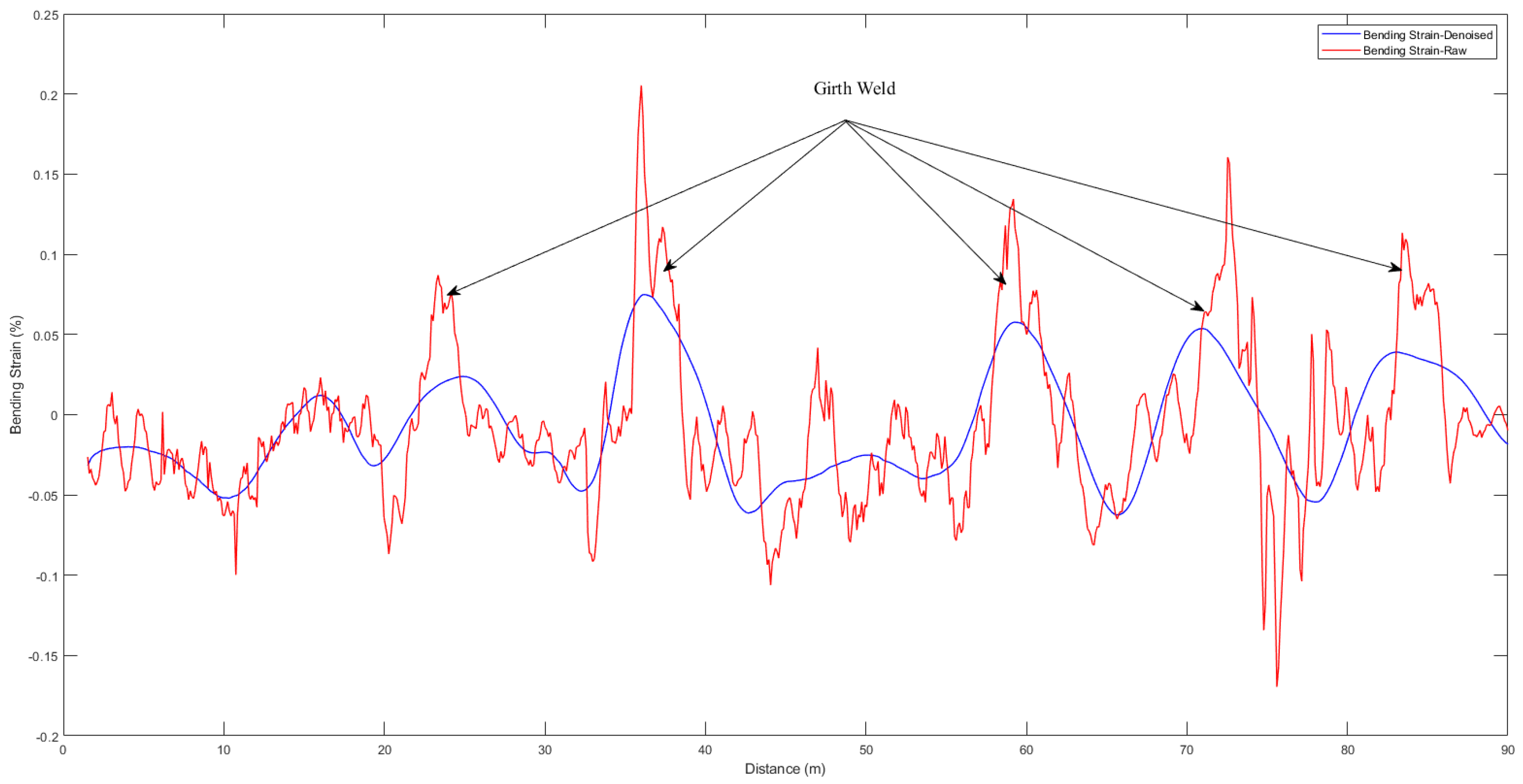
Data noise interferes with the features of the pipe section. Additionally, in the raw IMU strain data, jagged noises that fluctuate up and down owing to spiral welds and other reasons can be observed. During the process of the manual identification, some pipeline sections exhibit strain values greater than 0.125% only at a few points, but they are classified as bending strain sections. These points with large strain values may be caused by noise fluctuations, whereas it is not necessary to identify these sections when the noise is eliminated.

From the above-mentioned outcomes, it is obvious that pipeline bending strain inspection by using an IMU has become the most reliable technical means to obtain the strain of the entire pipeline. The various studies are still in the primary stage, and thus there are some defects and deficiencies. It is hence necessary to devise a new intelligence method for the identification accuracy of the specific anomaly features to further improve the identification efficiency and accuracy of the massive bending strain data.

Deep learning has achieved good results in image recognition, autonomous driving and other fields with its powerful feature extraction capabilities. The feature identification based on deep learning has the following advantages. Firstly, deep learning has powerful feature self-extraction ability, which can automatically extract features from original data, reduce the dependence on feature extraction technology. Secondly, the deep model can well discover the distribution of data and has a good nonlinear mapping ability to match the data with the state, which is very suitable for the feature recognition requirements in the context of big data. Many deep learning methods have been studied on pipeline defect identification. Aiming at the low efficiency of traditional methods for weld quality detection in industrial laser welding, Feng proposed a method for detecting weld defects on the surface of industrial steel plates based on convolutional neural networks, and the detection accuracy of weld defects can reach more than 97% [15]. Aiming at the problem that defects are difficult to identify in MFL (magnetic flux-leakage testing) inspection of petrochemical pipelines, Zhao established a three-dimensional finite element model for pipeline metal loss defects, and used three machine learning algorithms such as support vector machine, random forest and gradient boosting decision tree (GBDT) to classified and identified for defect signal. It is effective for the classification and identification of defects [16]. Wang proposes a pipeline defects diagnosis method based on deep learning neural network (DLNN). The average accuracy rate of pipeline defects identification is 92.86%, which has higher stability and identification rate than the BPNN method and SVM method [17]. Sun proposes a pipeline inner wall defect detection method based on pipeline robot and deep learning model algorithm, which can identify and classify pipeline inner wall defect images. The improved faster RCNN deep learning algorithm has the advantages of high recognition accuracy and low cost for pipeline defect recognition, and the average accuracy rate reaches 93.2% [18]. However, there are few research for pipeline bending strain inspection using deep learning methods. By considering the problems of the inconsistent discrimination standards, low identification efficiency, and high misjudgment rate during the application of the traditional manual identification methods, a feature identification method for the in-line inspected pipeline bending strain based on an optimized DBN model is proposed in this work. Our model utilizes deep learning methods to automatically extract feature signals from a large amount of data, while taking advantage of its strong feature identification ability to construct a DBN model with peak hold down sampling (PHDS) and particle swarm optimization (PSO) properties. Moreover, when the de-noised pipeline bending strain signal was used as the input of the DBN model, the PHDS method was employed for data compression, and the PSO algorithm was used to optimize the parameters of the model. Thereby, the training efficiency of the DBN model was significantly improved and the global optimization of the model parameters was realized. Thus, high identification accuracy was obtained to provide direct technical guidance for pipeline integrity management and excavation for maintenance.

2. Pipeline Bending Strain In-Line Inspection System and Bending Strain Calculation

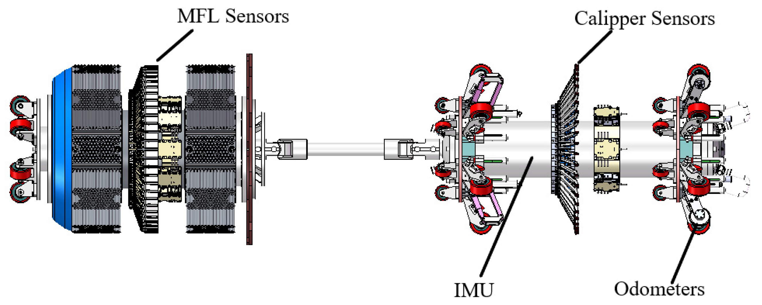
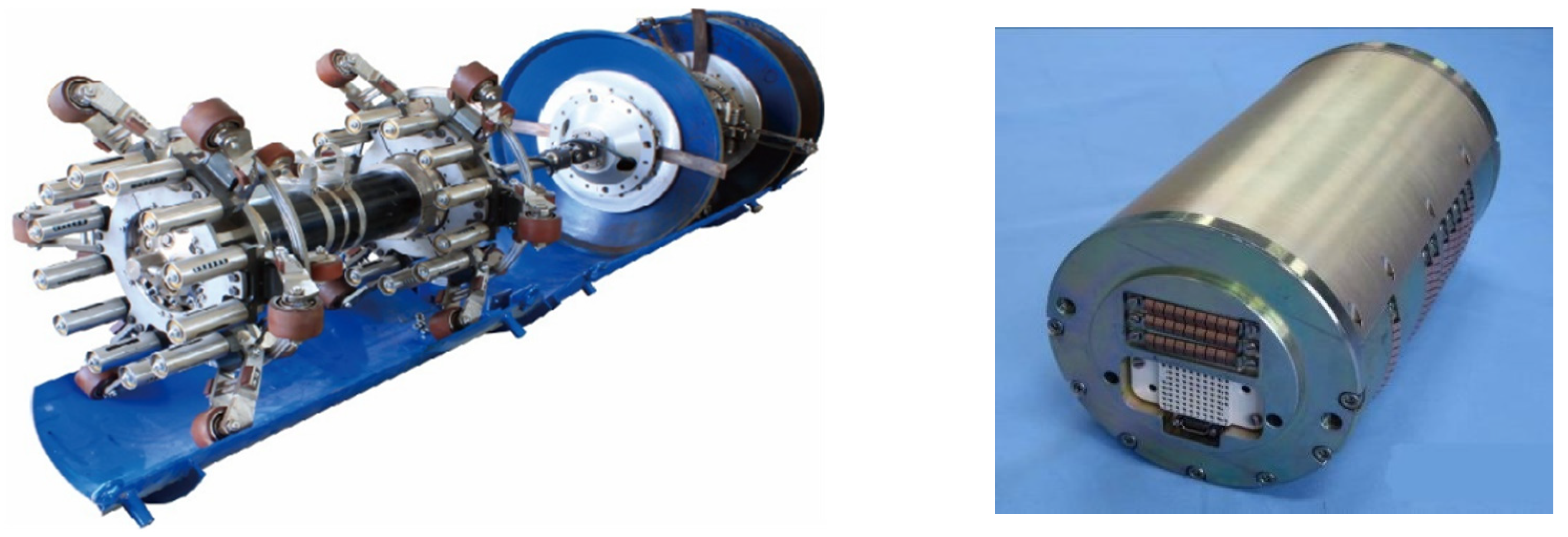
2.1. Composition of the Pipeline Bending Strain In-Line Inspection System

The employed pipeline bending strain in-line inspection system is an in-line tool based on an inertial navigation system (INS). Since the tool carries out inspection in the buried pipeline for a long time, it cannot be positioned in real-time through using the global positioning system (GPS) or BeiDou Positioning System [19,20]. Therefore, its operation strongly relies on the application of a high-precision inertial navigation system of the in-line tool to acquire the running attitude, speed, etc. In addition, the main component of the pipeline bending strain in-line inspection system is the inertial measurement unit (IMU), which is based on the strapdown inertial navigation technology. By considering that this component cannot run directly in the oil and gas pipeline, it needs to be sealed and mounted on the pipeline inspection tool. Within a confined space, the stability of the high-precision IMU gyroscope can reach 0.005°/h, with an attitude accuracy of 0.03° for heading and 0.01° for pitch and roll. As the coordinate data are collected by the sub-meter ground marker, the centerline coordinates of the pipeline and the attitude data of the in-line tool along the entire pipeline can be accurately calculated, and as a result, the bending strain can be also calculated. In addition to the capsule, the implementation of in-line tools also needs to be equipped with a series of sensors and auxiliary devices to enable the in-line tool to run safely within the oil and gas pipeline for a long time [21,22,23].

The structure of the pipeline bending strain in-line inspection system is schematically illustrated in Figure 1. It is mainly composed of in-line tools, inertial measurement devices, odometers, ground tracking systems, speed control units, battery management data storage units, and driving cups. Besides, to inspect metal loss, geometric deformation and other types of defects of the pipeline, various sensing elements are generally integrated into the tool, such as magnetic flux leakage (MFL) sensors and caliper sensors.

2.2. Calculation Method of the Pipeline Bending Strain

Generally, the bending strain distribution of a pipeline is directly related to its curvature [24]. Furthermore, in the centerline calculation of the pipeline, in addition to the pipeline coordinates, the attitude information of the corresponding in-line tool can be obtained, including the pitch angle, heading angle, and rolling angle. Hence, the curvature of the pipeline can be calculated first. It is interesting to notice that the change in the pitch angle of the tool represents the change in the inclination angle of the pipeline that is relative to the horizontal plane in the observed pipeline, while the heading angle represents the included angle between the tool running direction along the pipeline and the due north direction. The variations in the pitch angle and heading (ΔP and ΔA) are related to the length of the centerline of the observed pipeline (Δs), whereas the total curvature of the pipeline (k) and its vertical and horizontal components (K_v and K_h) are expressed as follows [25]:

$$\{\begin{array}{l}k=\sqrt{k_v{}^2+k_h{}^2}\\ k_v=\frac{\Delta P}{\Delta s}\\ k_h=-\frac{\Delta A}{\Delta s}\cos (P)\end{array}$$

(1)

If the centerline of the pipeline is assumed to be located on the neutral axis, the bending strain of the pipeline and curvature of the centerline have the following relationship:

$$\{\begin{array}{l}\epsilon =\frac{D}{2}k\\ {\epsilon }_v=\frac{D}{2}{k}_v\\ {\epsilon }_h=\frac{D}{2}{k}_h\end{array}$$

(2)

where D is the nominal diameter of the pipeline, $\epsilon$ stands for the total bending strain of the pipeline, and ${\epsilon }_v$ and ${\epsilon }_h$ denote the vertical and horizontal strain components, respectively.

Moreover, the total bending strain ε represents the maximum bending strain caused by the bending effect in the pipeline crossing area. The vertical strain component ${\epsilon }_v$ corresponds to the enforcement of the longitudinal strain at the bottom of the pipe (the values of the bending strain at both the top and the longitudinal strain at the top of the pipe are the same, while their signs are opposite). The horizontal strain component ${\epsilon }_h$ represents the value of the radial strain on the outermost right side of the pipeline (along the medium flow direction), and this value is the same as the respective value of the applied bending strain on the left side, which has the opposite sign.

2.3. Denoising of the Bending Strain Data

In the process of in-line IMU inspection of pipelines, the high-frequency interference noise exists in the IMU strain data due to the influence of the pipeline weld, dirt deposition, vibration of the tool, third-party interference, and other factors. Consequently, if the raw strain data are directly used for the feature extraction process, the noise features may be extracted together, resulting in the fuzzy identification of various types of pipeline features by using the machine learning model and reducing the identification accuracy of the machine learning model. Therefore, it is necessary to employ a scientific and reasonable method to remove the noise from IMU data. In the previously reported works, many methods were used to study the denoising the raw signals. J. Taler present an effective method which used seven- or nine-point moving average filters based on a local polynomial of third degree with respect to time in solving inverse heat conduction problems [26,27]. Jacek Wodecki reviewed the various methods for diagnostic data smoothing of Load-Haul-Dump machines [28]. These methods can be used fast and efficient to denoising the signals while preserving informative trends. Graham Horgan Wavelet verified the wavelet shrinkage as a highly adaptable method for signal smoothing by the simulation for time series showing gradual, rapid and discontinuous variations [29]. Rui Li proposed a method of measurement precision based on the implementation of a wavelet neural network that yields better repeatability and convergence than the original method [30].

The extracted results before and after pipeline bending strain denoising are shown in Figure 2. As can be ascertained, owing to the influence of weld and vibration on the pipeline, the calculated raw strain value of the pipeline at these characteristic points changes suddenly, which cannot truly reflect the overall strain pattern of the pipeline. The influence of these features can be eliminated by using wavelet denoising.

2.4. Pipeline Features Based on Bending Strain

During the process of IMU in-line inspection, a variety of pipeline feature signals are detected. In addition to the features of the pipeline section displacement caused by the enforcement of external forces that should be detected, other information will also be inspected. More specifically, the pipeline features that need to be classified mainly include the following:

(1)

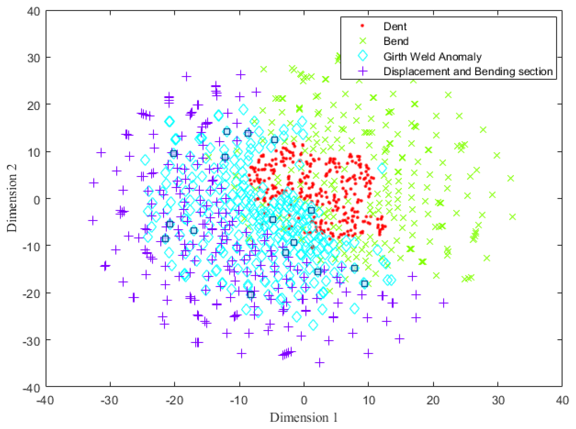
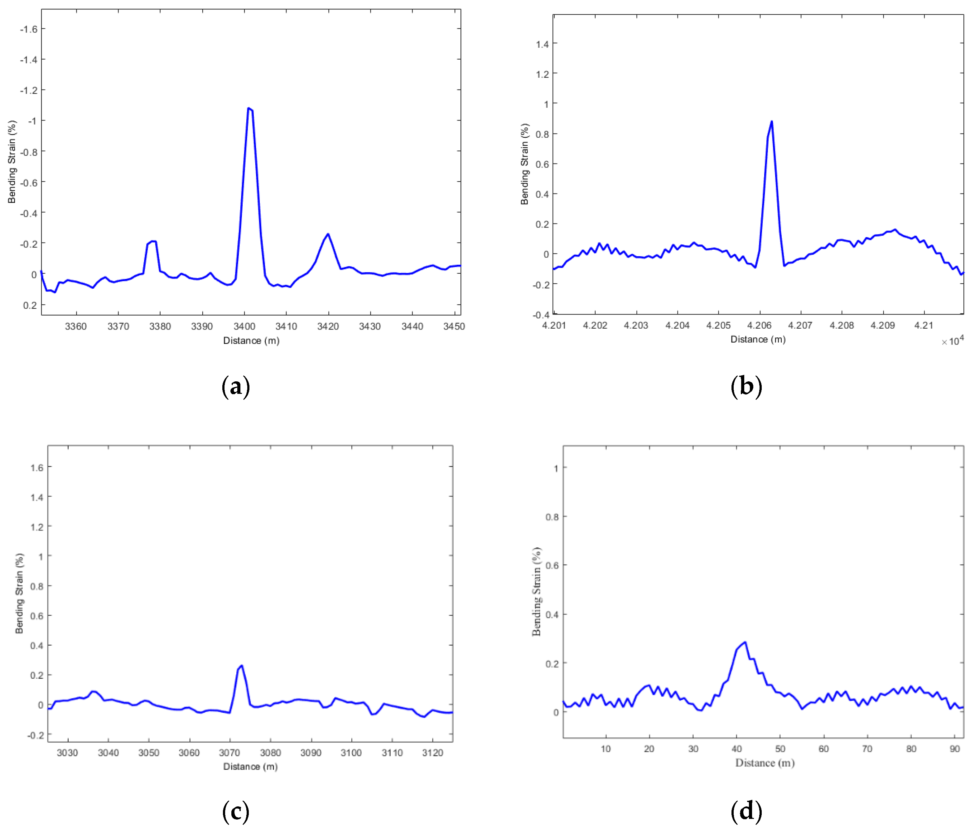
Dent: Figure 3a illustrates the strain signal of the pipeline dent. As a common defect form of pipelines, it seriously threatens the safe operation of the pipelines and even leads to pipe failure. We have to underline that the pipe dent effect refers to the local elastic-plastic deformation where an obvious change in the pipe surface curvature is caused by an external impact or extrusion. On top of that, during the construction and operation of the pipeline, owing to the extrusion of hard and big objects such as rocks and the collision of excavating equipment and falling rocks, both the bottom and top of the pipeline may be dented.

(2)

Bend: Figure 3b divulges the strain signal of the pipe bend. Since pipelines are the main equipment for transporting fluid medium in the petroleum industry, bends must be used to adjust the transmission direction of the pipeline or connect two pipes whose central axis is not aligned due to the limitation of space or design route. The commonly used bends are 45°, 90°, and 180°, and bends of 60°, and other unconventional angles are also used according to the engineering needs.

(3)

The girth weld anomaly of the pipeline: Figure 3c reveals the strain signal of the girth weld anomaly of the pipeline. Moreover, long-distance oil and gas pipelines are generally made of a large number of factory-manufactured straight pipes that are connected with accessories (bends, tees, valves, etc.). Since the welded joints are not only firm and durable, but also have high joint mechanical strength and tightness, they are the most commonly used for the fabrication of important pipeline connection modes in pipeline construction projects. It is interesting to notice that when the in-line tool runs in the pipeline, due to the abnormality of some girth welds (miter joint, excessive reinforcement, staggered edge, etc.), the in-line tool is subjected to a large impact and vibration loads at the girth weld anomalies, so the information of these girth welds also needs to be distinguished.

(4)

The bending deformation section: Figure 3d reveals the strain signal of the bending deformation of the pipeline. Due to the nature of the employed long-distance oil and gas pipelines, they often pass through areas with unstable geological conditions or natural disasters, such as earthquake areas and frozen soil areas. As a result, in these areas, large lateral displacement and deformation on the pipeline is easier to be imposed, and in severe cases, a large bending strain will be generated locally. Therefore, these bending deformation features need to be effectively identified by using an in-line IMU inspection method.

3. Feature Identification Method for the In-Line Inspected Pipeline Bending Strain Based on Optimized DBN Model

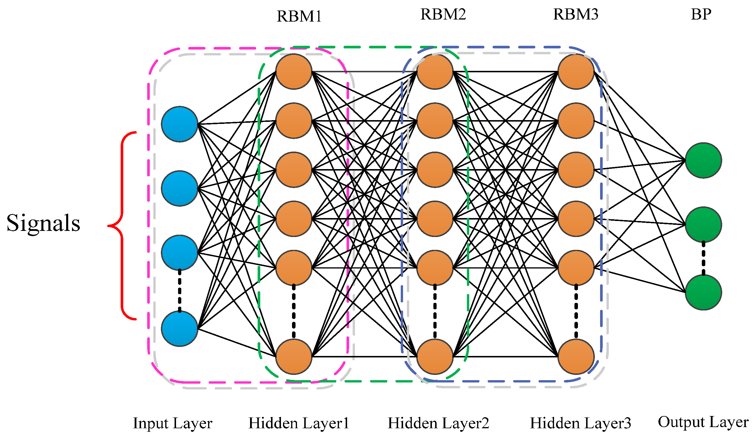
The DBN model can learn and obtain high-level main features directly from the low-level original signals layer by layer and realize both state identification and classification. Additionally, DBN eliminates the process of manual feature extraction, integrates feature extraction and classification, and avoids the complexity and incompleteness of the feature extraction. Since the original signal is employed as the input of the DBN, to ensure that the data sample contains sufficient state information, the sample data should have a certain length, which leads to an increase in the model training time. To address this issue, it is necessary to compress the sample data, reduce the sample length, and decrease the amount of computation on the premise of preserving the signal state information as much as possible. As far as the problems where it is difficult to determine the DBN model parameters are concerned, especially the number of the RBM layers and the number of neurons in each layer, the parameter optimization algorithm is used to find the optimal model parameters and get rid of the uncertainty of relying on “trials”.

3.1. DBN Theory

The DBN is composed of multilayer restricted Boltzmann machines (RBMs) and a layer of back propagation (BP) neural network (as is shown in Figure 4). The training process was divided into pre-training and fine-tuning. The pre-training trains all RBMs in an unsupervised manner, whereas fine-tuning is used to fine-tune the weight and bias parameters of the pre-trained model through the implementation of the BP algorithm [31,32].

(1)

Pre-training

The DBN is mainly composed of RBMs and is derived from the energy model of thermodynamics [33]. Furthermore, RBMs can be found in two layers: the upper layer is the hidden layer and the lower layer is the visible layer. The energy function of the RBM model is defined by the following equation:

$$E\left(v,h|\theta \right)=-{\displaystyle \sum _{i=1}^I{a}_i{v}_i}-{\displaystyle \sum _{j=1}^J{b}_j{h}_j}-{\displaystyle \sum _{i=1}^I{\displaystyle \sum _{j=1}^J{w}_{ij}{v}_i{h}_j}}$$

(3)

where I and J denote the number of nodes in the visible and hidden layers, respectively, $v=\left(v_1,v_2\cdots ,v_i\right)$ and $h=\left(h_1,h_2\cdots ,h_j\right)$ represent the states of the visible layer and the hidden layer, respectively, $\theta =\left\{w_{ij},a_i,b_j\right\}$ stand for the model parameter of the RBM model, $w_{ij}$ is the weight of the ith neuron of the visible layer and the jth neuron of the hidden layer, $a_i$ signifies the bias of the ith node of the visible layer, and $b_j$ is the bias of the jth node of the hidden layer.

According to the energy function of the employed RBM model, the joint probability distribution of the visible and hidden layer states $\left(v,h\right)$ can be obtained as follows:

$$p\left(v,h|\theta \right)=e^{-E\left(v,h|\theta \right)}/Z\left(\theta \right)$$

(4)

where $Z\left(\theta \right)={\displaystyle \sum _{v,h}{e}^{-E\left(v,h|\theta \right)}}$ is the mean normalization factor.

The probability of the hidden node h_j and the visible node v_i being activated is:

$$P\left(h_j|v\right)=\sigma \left(b_j+{\displaystyle \sum _{i=1}^I{W}_{ij}{v}_i}\right)$$

(5)

$$P\left(v_i|h\right)=\sigma \left(a_i+{\displaystyle \sum _{j=1}^J{W}_{ij}{h}_j}\right)$$

(6)

where $\sigma (\cdot )$ is the activation function.

To enable the neural network to solve complex problems, it is necessary to add nonlinear factors to the neural network through the activation function.

When training the RBM, the maximum likelihood method is employed to obtain the parameter set $\theta =\left\{w_{ij},a_i,b_j\right\}$, and the training data are used to train the RBM to obtain the maximum likelihood function is expressed as follows:

$$L(\theta )={\displaystyle \prod _{l=1}^{N}L(v|\theta )={\displaystyle \prod _{l=1}^{N}p(v)}}$$

(7)

where N is the number of samples. The random gradient rise method is also used to calculate the derivation of the parameters of the maximum likelihood function, including the weight and bias of each node, that is,

$$\frac{\partial \ln L}{\partial w_{ij}}={\displaystyle \sum _{l=1}^N[P(h_j}=1|v^l)v_i^l-{\displaystyle \sum _{v}P(v)P(h_j}=1|v)v_i]$$

(8)

$$\frac{\partial \ln L}{\partial a_i}={\displaystyle \sum _{l=1}^N[}{v}_i^l-{\displaystyle \sum _{v}P(v)}{v}_i]$$

(9)

$$\frac{\partial \ln L}{\partial b_j}={\displaystyle \sum _{l=1}^N[P(h_j}=1|v^l)-{\displaystyle \sum _{v}P(v)P(h_i}=1|v)]$$

(10)

The parameters are consequently updated to obtain the state of the visible neuron node through the state transition between the visible layer and the hidden layer several times, to fit the sample with the maximum probability, which not only reduces the frequency of the state transition, but also improves the computational efficiency. To attain this goal, the basic steps are to set the training set as the state of the visible neuron node and calculate the state of all of the hidden neuron nodes. Interestingly, when the state of the hidden neuron node is determined, the state of the visible neuron node is reconstructed, and then the parameters are updated by using the error between the state of the visible neuron node and the state of the reconstructed visible neuron node several times, which greatly enhances the computational efficiency of RBM.

(2)

Fine-tuning

RBM pre-training is an unsupervised learning scheme. The model parameters that are obtained from the pre-training process are regarded as the initialization of the DBN model parameters. Fine-tuning involves the gradual fine-tuning of the DBN model parameters by using a back-propagation algorithm starting from the BP layer through the sample labels to further optimize the model. Along these lines, the SoftMax function is often used as a classifier model in the last layer of the DBN. If we consider that the data sample is x, and the DBN includes l layers of RBMs, and assume that the output vector of the last layer of RBMs is $u_l\left(x\right)$.

$$u_l\left(x\right)=W_l{u}_{l-1}\left(x\right)+b_l$$

(11)

$$\stackrel{\wedge }{X}=\mathrm{softmax}\left(u_l\left(x\right)\right)$$

(12)

where $u_l\left(x\right)$ is the output of the lth layer, $W_l,b_l$ stand for the weight and bias of the lth layer, $\stackrel{\wedge }{X}$ represents the output of the last layer of the network, and Softmax signifies the activation function of the last layer.

The mean square error is also used as a function of loss, while the error back propagation algorithm based on the principle of the minimum mean square error is employed to update the parameters of the entire network. The loss function is expressed as follows:

$$loss=\frac{1}{N}{{\displaystyle \sum _{i=1}^N\left(\stackrel{\wedge }{X_i}-X_i\right)}}^2$$

(13)

where loss is the mean square error of the forward propagation, and $\stackrel{\wedge }{X_i}$ and $X_i$ represent the output and expected output, respectively, of the output layer. The basic concept of DBN training is to fully train the first RBM model after preprocessing the training set and after fixing the first RBM parameters, while the second RBM model is trained with the first RBM hidden neuron state as input, and then train all RBMs layer by layer. In addition, the hidden neuron state of the last RBM is introduced as input into the regression layer, while the output value is compared with the expected value, and the parameters of the entire model are fine-tuned by using the error back propagation algorithm.

3.2. Peak Hold Down Sampling (PHDS) Algorithm

When the DBN diagnosis model of a gas turbine rotor system is constructed, owing to the large length of the input sample data, the model training speed is relatively low. As a result, to reduce the model training time, the sample length should be compressed as much as possible under the condition of guaranteeing the state information of the sample data [34]. Besides, the basic idea of the PHDS algorithm is to segment the signal with a high sampling rate through a fixed down sampling ratio, and reconstruct the signal by taking the peak of each segment of the signal as the resampling value. We have to underline that this method not only reduces both the data and the amount of computation, but also has an obvious effect on preserving the features of the signal. It is also assumed that the collected gearbox vibration signal $s(t)$ is a signal segment containing N points, whereas the sampling frequency is $f_0$.

$$E\left(v,h|\theta \right)=-{\displaystyle \sum _{i=1}^I{a}_i{v}_i}-{\displaystyle \sum _{j=1}^J{b}_j{h}_j}-{\displaystyle \sum _{i=1}^I{\displaystyle \sum _{j=1}^J{w}_{ij}{v}_i{h}_j}}$$

(14)

$$s\left(t\right)=[t_0,t_1,\cdots ,t_i,\cdots ]\begin{array}{cc}& \end{array}\left(0\le i\le N-1\right)$$

(15)

By dividing $s(t)$ into M data segments, and the signal $s(t)$ is transformed into $S\left(T\right)$, then $S\left(T\right)$ can be expressed as follows:

$$S\left(T\right)=\left[S\left(T_0\right),S\left(T_1\right),\cdots S\left(T_j\right)\cdots \right]\begin{array}{cc}& \end{array}\left(0\le j\le M-1\right)$$

(16)

$$S\left(T_j\right)=[t_{rj},t_{rj+1},\cdots ,t_{rj+r-1}]$$

(17)

where N is the length of the original signal, and r represents the downsampling rate, which is defined as the data reduction rate, $M=N/r$. After the peak value of the data as downsampled, the sampling frequency is $f_d=f_0/r$. To ensure that the state information of the compressed data is not seriously lost as much as possible, the down-sampling frequency is generally set from 2 to 4

Then, the maximum value of the acquired absolute values of the values in the sequence $S\left(T_j\right)$ is extracted as the reserved value to represent the sequence $S\left(T_j\right)$, and the maximum values of the absolute values of the values in all data segments are rearranged to obtain the signal sequence after downsampling.

3.3. Particle Swarm Optimization Algorithm (PSO)

As far as the DBN model is concerned, the main factors affecting the performance of the DBN are the number of the RBM layers in the model and the number of neurons in each layer. Thus, the more DBN hidden layer networks, the easier it is to obtain the features of the raw data. However, with the increase of the hidden layer networks, over-fitting occurs easily, and the diagnostic accuracy decreases [35,36]. Therefore, the selection of the appropriate model parameters is important for the model performance. In addition, if all possibilities are listed by an exhaustive method, they will consume a lot of time. Interestingly, the parameter setting of the DBN model most relies on empirical rules, which are prone to local optimization problems. Therefore, it is very important to achieve a global optimization process of the DBN model parameters.

Under this direction, particle swarm optimization is an intelligent optimization algorithm. More specifically, this algorithm is derived from the simulation of the predation behavior of birds, whereas the position of each particle is the parameter corresponding to the optimal solution of the population. Through the cooperation and the information interaction between individuals and groups, the population evolution is completed, and the optimal solution of the nonlinear problem is obtained. A D-dimensional search space is set and the following expression is used $X=(X_1,X_2,\dots ,X_M)$ to represent the population, while the position of the ith particle for the kth time is represented by $X_i^k=(X_{i1}^k,X_{{}_{i2}}^k,\dots ,X_{iD}^k)$, and the velocity of the ith particle for the kth time is represented by $V_{{}_i}^k=(V_{i1}^k,V_{{}_{i2}}^k,\dots ,V_{{}_{iD}}^k)$. The optimal position of particles is represented by $P_i=(P_{i1},P_{i2},\dots ,P_{iD})$, whereas the optimal position of the groups is denoted by $P_g=(P_{g1},P_{g2},\dots ,P_{gD})$. The specific process of the PSO algorithm is represented as follows. Firstly, random values are assigned to both the position and velocity of each particle. Then according to the preset objective function, the fitness of each particle can be calculated and both the advantages and disadvantages of its position can be evaluated. Finally, both the velocity and position are updated according to the results of each iteration, and the global optimal solution is obtained after performing multiple iterations.

$$V_{id}^k=W{V}_{id}^{k-1}+c_1{r}_1\left(p_{id}-x_{id}^{k-1}\right)+c_2{r}_2\left(P_{gd}-x_{id}^{k-1}\right)$$

(18)

$$x_{id}^k=x_{id}^{k-1}+v_{id}^{k-1}$$

(19)

where c₁ and c₂ represent the acceleration factors, and r₁ and r₂ are random numbers with a value in the range of (0,1).

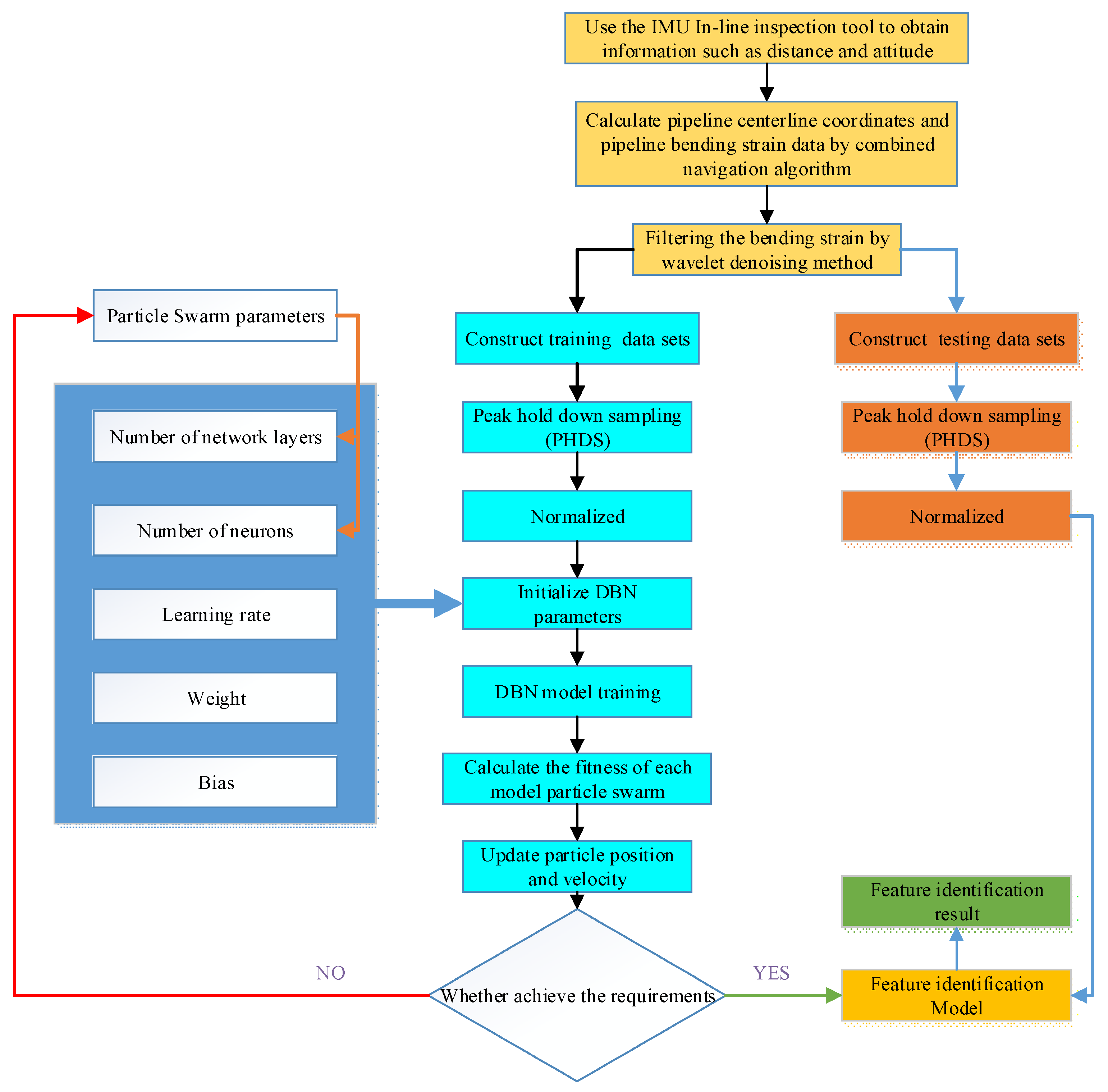
3.4. Pipeline Bending Strain Feature Identification Method Based on Improved DBN with Particle Swarm Optimization

To address the problem of the long training time of DBN, the PHDS algorithm was used to compress the sample data, reducing the sample length and the amount of computation based on preserving the signal state information as much as possible. At the same time, by considering the difficulty in determining the model parameters of the DBN, such as the number of the RBM layers in the model and the number of neurons in each layer, the PSO algorithm was used to search the optimal model parameters of the DBN model to get rid of the uncertainty of relying on “trials”. Furthermore, a flowchart of the proposed model is disclosed in Figure 5. The training process of the fault diagnosis model based on the improved DBN includes the following steps.

(1)

The data sample set was constructed with the de-noised signals obtained through the calculation of the pipeline bending strain, including both the training data sample set and the test sample set. The PHDS method was also used to compress the data samples. To ensure that the state information of the compressed sample data is not seriously affected, the downsampling rate is generally 2–4.

(2)

The compressed data samples were normalized through the range method $x_{out}=\left(x_{in}-x_{\min }\right)/\left(x_{\max }-x_{\min }\right)$, to obtain the ratio of the result of a segment of signal data minus the minimum value to the result of the maximal value minus the minimum value.

(3)

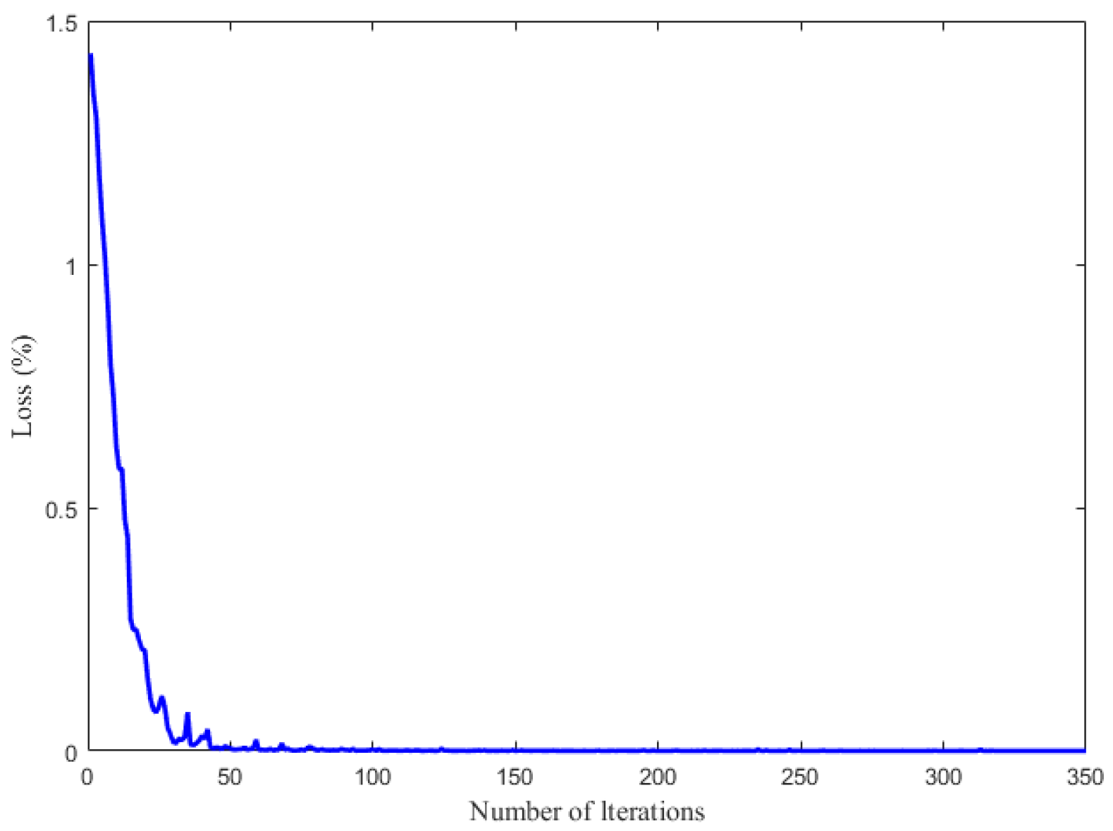
Consequently, the weight of the DBN is set, and the bias parameter is initialized immediately. Additionally, the loss function is the mean square error, the activation function is the sigmoid function, the learning rate is set to 0.1, the number of iterations is set to 50, the number of the network layers is an integer between 1 and 4, and the number of neurons in each layer of the network is initialized immediately.

(4)

The training sample set is loaded, then the PSO algorithm is used, and the test accuracy of the test data model is taken as the objective function to search the number of the network layers while the number of neurons in each layer of the model with the highest test accuracy of the test data.

(5)

According to the number of the network layers and the number of neurons in each layer, the optimal DBN model is constructed for the studied object, and the feature classification process based on bending strain is realized by using the DBN model.

4. Field Experimental Investigation

4.1. Data Preparation for Field Experiment

A crude oil pipeline with a length of 999.04 km, outer diameter of 813 mm, main pipeline section wall thickness of 11.9 mm, design pressure of 8 MPa, pipeline material of L450 (X65) steel, and transported medium of crude oil was employed. The pipeline passes through seasonally frozen soil. Owing to the thawing and sinking of the seasonally frozen soil, the pipeline is prone to the enforcement of large bending deformation, which seriously threatens the normal operation of the pipeline. The IMU in-line tool was also used to inspect the pipeline to inspect the bending deformation of the entire pipeline. Figure 6 depicts the IMU in-line tool and the high-precision inertial navigation unit.

According to the statistical results of the strain data detected by in-line IMU for many years, a total of 3200 samples of four types of features, namely dent, bend, girth weld anomaly, and bending and displacement were extracted as samples, which were subsequently divided into 2000 training samples and 1200 test samples. On top of that, the t-distributed stochastic neighbor embedding (t-SNE) [37,38] can be used to reduce the dimensions of data and realize a two-dimensional visualization to observe the distribution of the sample data and determine whether it is possible to be classified. More specifically, the divided training sample datasets were reduced to two dimensions by using the t-SNE method to obtain a two-dimensional distribution map of the training samples. Figure 7 illustrates the two-dimensional visualization of the pipeline features before applying the identification procedure, while it can be found that the training sample set exhibits a certain clustering and thus can be classified.

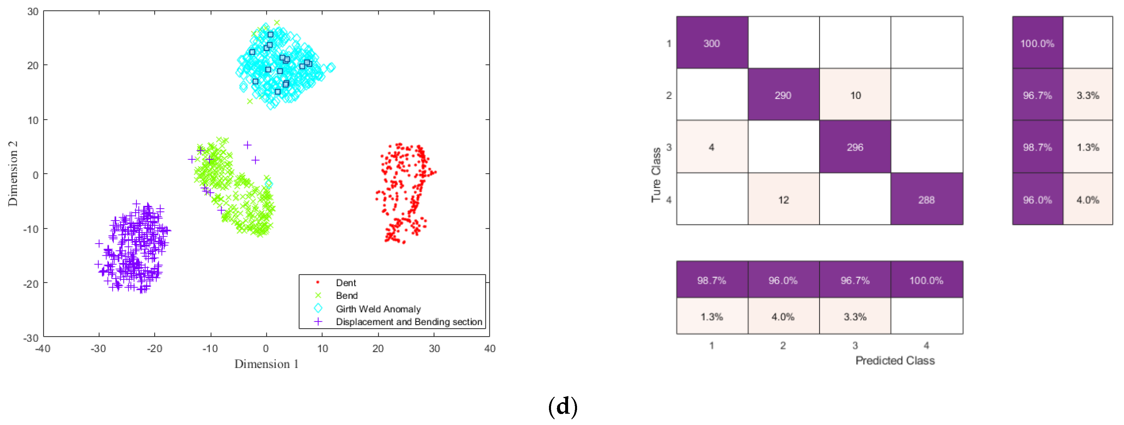
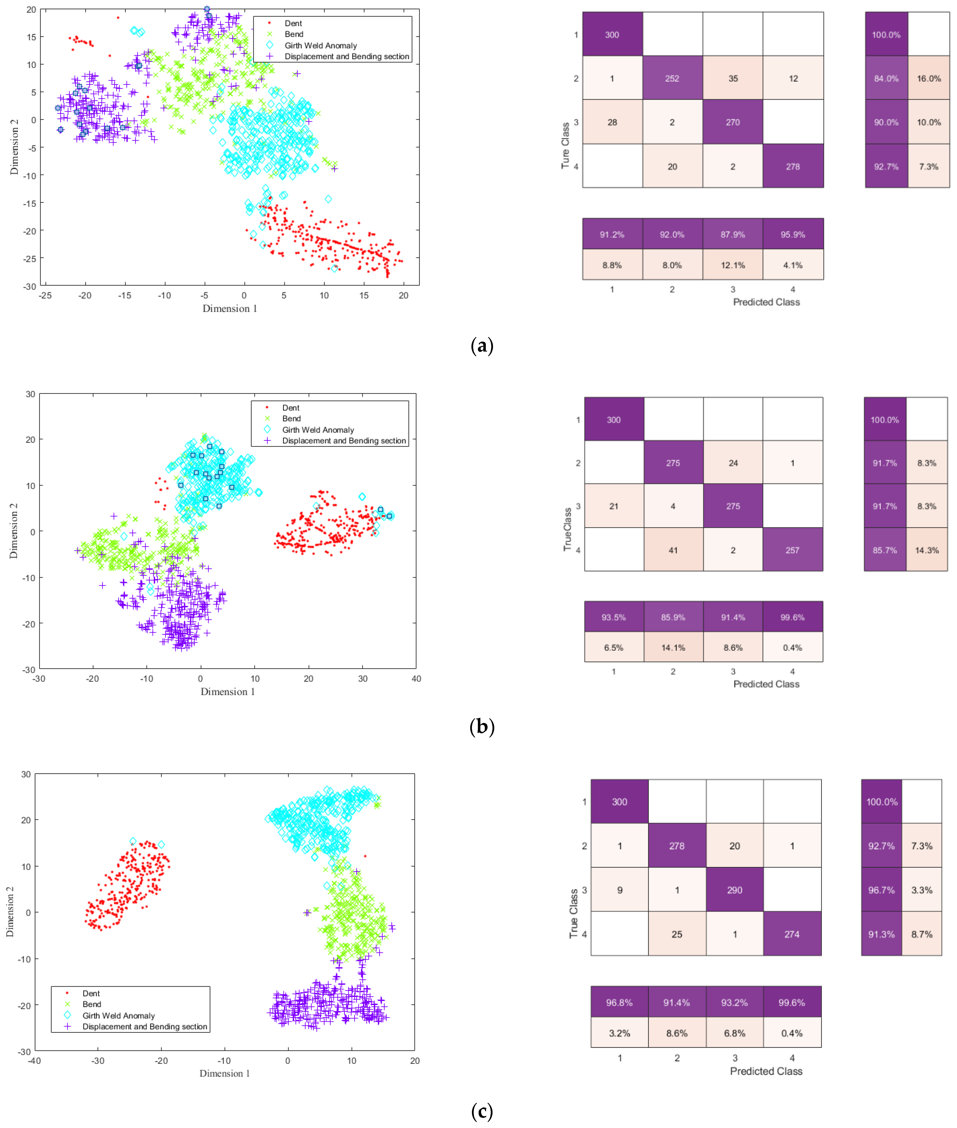
4.2. Pipeline Feature Classification Based on the Improved DBN

The PHDS algorithm was used to compress the sample data. For the sample data with different reduction ratios, the DBN models that were optimized by the PSO algorithm were constructed, while the optimal models corresponding to the reduction ratio were obtained. The compressed test data were also employed to test the impact of the downsampling rate of the PHDS algorithm on the model training, whereas the acquired test results are presented in

Table 1. Test results of the PHDS method.

Category	Down Sampling Rate	Sample Length	Model Training Time	Test Accuracy
1	1	2048	176 s	97.95%
2	2	1024	142 s	97.83%
3	4	512	130 s	90.1%
4	8	256	81 s	82.8%
5	16	128	47 s	55.4%
6	32	64	28 s	43.6%

.

As is shown in Table 1, when the PHDS method is adopted to compress the sample, most of the state information in the sample can still be retained. However, when the reduction ratio is too large, the state information of the sample will be lost. As a result, to balance the training efficiency and model diagnosis impact, the reduction ratio was set to 2, and for the compressed sample data length 1024 data points were selected.

The compressed data samples were loaded to train the DBN, and the accuracy of the test data was taken as the objective function. The number of the PSO algorithm parameters was set as 10, the acceleration factor was set to 20, and the number of iterations was set to 20. The PSO algorithm was used to iteratively search for the optimal number of network layers and the hidden elements of the DBN model. After approximately carrying out 18 iterations, the optimal network model parameters were found. More specifically, the number of the hidden layers was two, and the number of neurons in the hidden layer was 100 and 100, respectively. The highest test accuracy of the model was 97.83%. Therefore, the DBN network structure is set to 1024-100-100-4.

From Figure 8, it can be seen that the accuracy becomes bigger with an increase in the number of iterations. On top of that, as can be observed from Figure 9, the loss function decreases with an increase in the number of iterations. It is also interesting to notice that when the number of iterations reached the value of 80, the test accuracy of the model and the loss function did not change. In addition, the highest test accuracy of the model of 97.83% was achieved, and a balance was reached between the model training efficiency and the model performance. If the number of iterations increases continually, the model training time increases.

The optimal network model parameters were found after approximately carrying out 80 iterations, whereas the DBN network with a structure of 1024-100-100-4 was used, and the bending strain data of approximately 260 km of pipeline laid in 2013 were selected for intelligent feature identification. Moreover, the time of the machine learning identification method was less than 5 min, which indicates that the identification efficiency was less than 0.02 min/km. As far as the manual identification method is concerned, the identification efficiency of professional engineers and technicians with rich experience in integrity evaluation is about 30 min/km. By using the proposed method, both the classification accuracy and identification efficiency improved significantly.

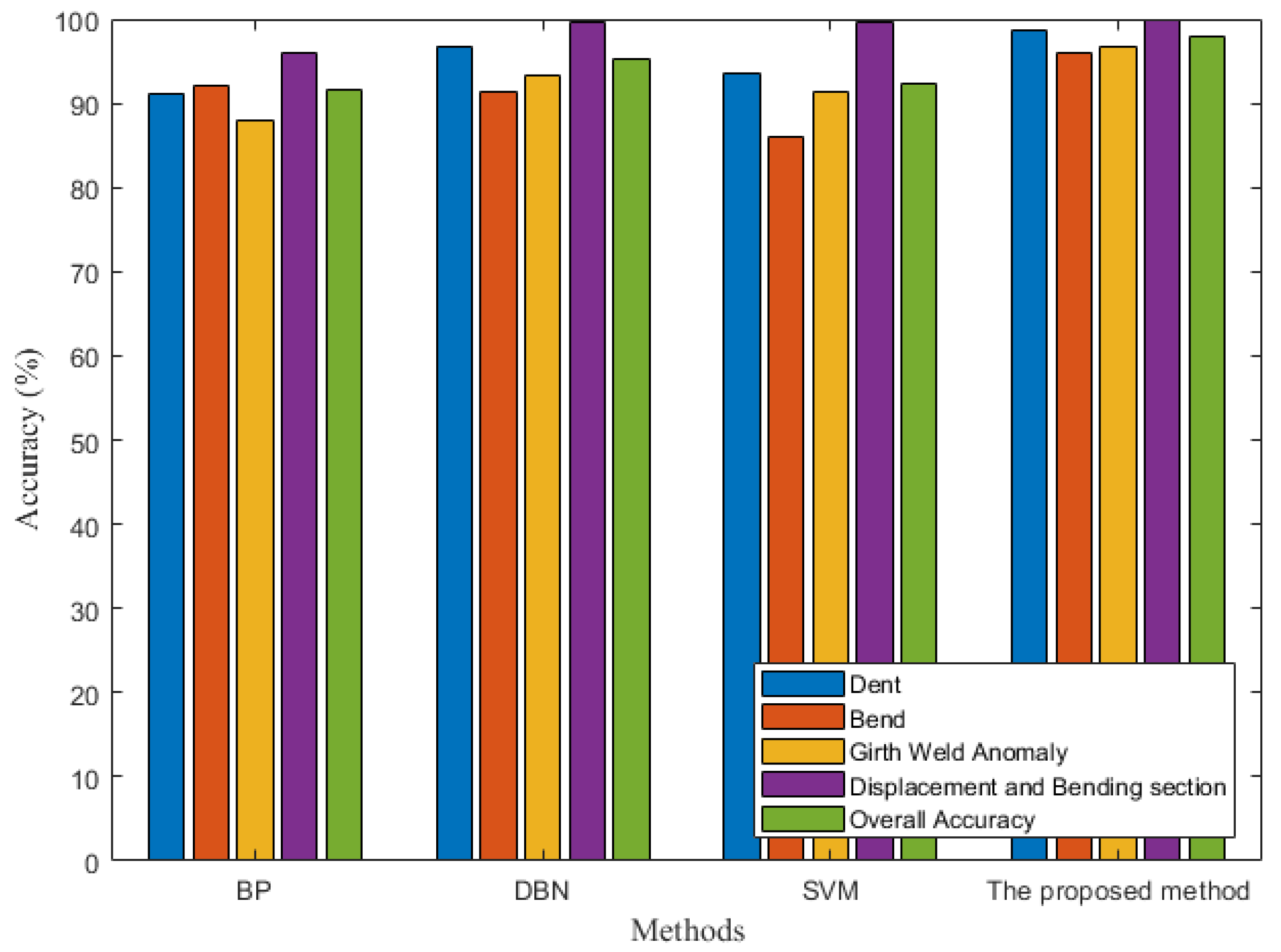
4.3. Comparisons with Other Methods

To compare the influence of the different methods on the pipeline feature identification process, other feature identification methods were compared with the proposed method.

(1)

BP neural network: the BP neural network is practically a multi-layer feedforward neural network, which is characterized by the signal forward transmission and error back propagation. During the forward propagation process, the input signal is processed from the input layer to the output layer through the hidden layer. The neuron state of each layer affects only the neuron state of the next layer. Consequently, if the output layer cannot obtain the expected output, it will turn back propagation and adjust the network’s weight and threshold according to the prediction error to continuously approach the expected output of the BP neural network.

(2)

Support vector machine (SVM): a support vector machine (SVM) method is proposed based on statistical learning theory. It is widely used in both pattern recognition and classification approaches due to its faster training convergence rate, stronger generalization ability than neural networks, and the ability to solve small sample learning problems.

(3)

DBN: the DBN is adopted for comparison with the proposed method.

Table 2. Accuracy comparison of the different methods.

Category	Model	Training Time (s)	Test Accuracy (%)
1	BP	96	91.6 (1100/1200)
2	SVM	118	92.25 (1107/1200)
3	DBN	128	95.17 (1142/1200)
4	Proposed method	142	97.83 (1174/1200)

and Figure 10 show the acquired classification results of the different methods. When the BP network was employed for feature identification, the classification accuracy was 91.6%. On the other hand, when the SVM network was used for feature identification, the classification accuracy was 92.25%. Finally, when a non-optimized DBN network was used for feature identification, the extracted classification accuracy improved to 95.17%. Hence, we can draw the conclusion that the proposed method in this work has a classification effect that is significantly higher than that of the other methods, while a classification accuracy of up to the value of 97.83% has been attained.

To more intuitively present the feature identification accuracy of the different methods, t-SNE and a confusion matrix were used to illustrate the various identification results. As a result, Figure 11 shows the identification results of pipeline features by using the BP neural network, SVM, DBN, and the method proposed in this work.

The t-distributed random neighborhood embedding (t- SNE) method is used to reduce the extracted feature dimension to 2D to reveal the final 2D feature representation of the test set, as shown in Figure 11. The results of each model are intuitively displayed in the figure, and the classification results of each model can be analyzed in detail through the confusion matrix. It can be seen from Figure 11a that BP neural network can identify most feature types, and the identification of dent, bend and bending section are 91.2%, 92%, and 95.9%, respectively, but the girth weld anomaly is 87.9%. As can be seen from Figure 11b, SVM can recognize most feature types, and the identification of dent, girth weld anomaly, and bending section are 93.5%, 91.4%, and 99.6%, respectively. The identification of bending section is only 85.9%. It can be seen from Figure 11c that DBN can improve the feature identification, and the identification of dent, bend, girth weld anomaly, and bending deformation are 96.8%, 91.4%, 93.2%, and 99.6%, respectively. As can be seen from Figure 11d, the feature identification of the proposed method in this paper is the best. The feature identification for four features are 98.7%, 96.7%, 96.7%, and 100%, respectively. Since there is a small bend signal in the samples, which overlaps with some girth weld anomaly, the misjudgment will occur in the process of feature identification.

From the overall effect of identification, it can be seen that by enforcing the BP neural network and SVM method, the pipeline features after performing the classification procedure are confused and not completely distinguished. Additionally, the classification results were improved by DBN, and the four types of features were almost completely separated by the improved DBN. Therefore, the classification results obtained by using the improved DBN are the best.

5. Conclusions

The stress state of long-distance oil and gas pipelines currently has evolved into an important problem for pipeline operators. Under this perspective, the high-precision IMU in-line inspection method makes it possible to detect the development of additional bending stresses in pipes. To quickly and accurately identify the features of the bending strain signals that are applied to the pipeline, a DBN model optimized by PHDS and PSO was constructed and used for feature identification based on the in-line inspection data in this work, which achieved a good feature identification outcome. The main contents and innovations of this work are as follows.

(1)

The wavelet denoising method can effectively remove the interference and noise of the bending strain data in pipeline detection, which lays a foundation for pipeline feature identification.

(2)

The PHDS method was used to compress the sample data, which can improve the identification speed to ensure elevated identification accuracy.

(3)

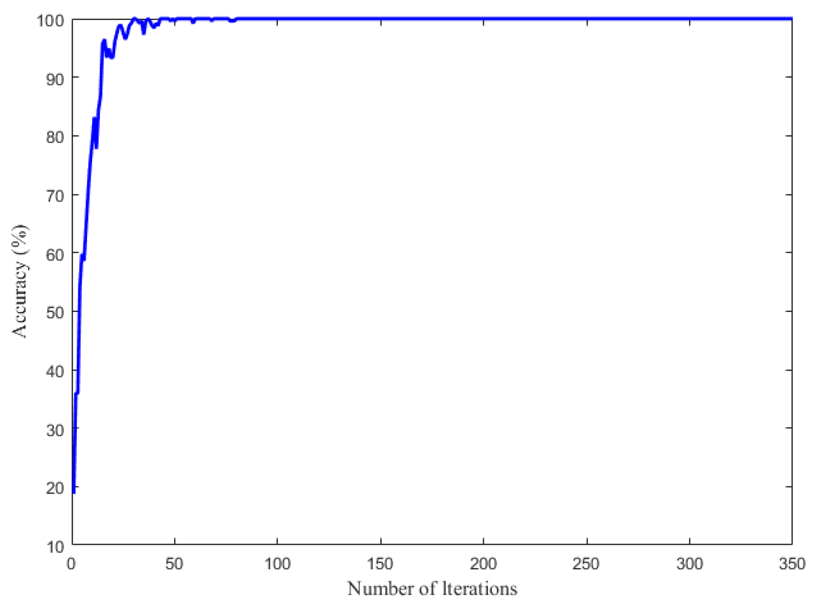
The PSO algorithm was adopted to optimize the parameters of the DBN model, which improves the training efficiency of the network model, realizes the global optimization of model parameters, and obtains a high test accuracy. The acquired application results show that the accuracy of pipeline feature identification based on the bending strain can reach the value of 97.83%, and the identification efficiency can reach 0.02 min/km.

References

1. DONG, S.H. Review of China’s oil and gas pipeline integrity management in the past 20 years and development suggestions. Oil Gas Storage Transp. 2020, 39, 241–261. [Google Scholar]
2. Wang, J.; He, R.; Liu, Z.; Hao, G. Development status of oil & gas pipeline integrity management standards in China and the USA and their differences. Oil Gas Storage Transp. 2017, 36, 1–10. [Google Scholar]
3. Taylor, P.; Wielki, J.; Shea, T. Incorporating Environmental Considerations into Pipeline Integrity Management Programs. In International Pipeline Conference; American Society of Mechanical Engineers: Calgary, AB, Canada, 2012; pp. 307–316. [Google Scholar]
4. Tejedor, J.; Martins, H.F.; Piote, D.; Macias-Guarasa, J.; Pastor-Graells, J.; Martin-Lopez, S.; Guillen, P.C.; De Smet, F.; Postvoll, W.; Gonzalez-Herraez, M. Toward Prevention of Pipeline Integrity Threats Using a Smart Fiber-Optic Surveillance System. J. Lightwave Technol. 2016, 34, 4445–4453. [Google Scholar] [CrossRef] [Green Version]
5. Feng, Q.; Li, R.; Nie, B.; Liu, S.; Zhao, L.; Zhang, H. Literature Review: Theory and Application of In-Line Inspection Technologies for Oil and Gas Pipeline Girth Weld Defection. Sensors 2017, 17, 50. [Google Scholar] [CrossRef]
6. Hussein, S.; Naser, E.S. A Novel Method to Enhance Pipeline Trajectory Determination Using Pipeline Junctions. Sensors 2016, 16, 567. [Google Scholar]
7. Liu, S.; Zheng, D.; Li, R. Compensation Method for Pipeline Centerline Measurement of in-Line Inspection during Odometer Slips Based on Multi-Sensor Fusion and LSTM Network. Sensors 2019, 19, 3740. [Google Scholar] [CrossRef] [Green Version]
8. Li, R.; Cai, M.; Shi, Y.; Feng, Q.; Chen, P. Technologies and application of pipeline centerline and bending strain of In-line inspection based on inertial navigation. Trans. Inst. Meas. Control 2018, 40, 1554–1567. [Google Scholar] [CrossRef]
9. Li, R.; Wang, Z.; Chen, P. Development the method of pipeline bending strain measurement based on microelectro mechanical systems inertial measurement unit. Sci. Prog. 2020, 103, 0036850420925231. [Google Scholar] [CrossRef]
10. James, D.; Hart, J.; Czyz, A.; Zulfiqar, N. REVIEW OF PIPELINE INERTIAL SURVEYING FOR GROUND MOVEMENT-INDUCED DEFORMATIONS. In Proceedings of the Conference on Asset Integrity Management-Pipeline Integrity Management Under Geohazard Conditions, AIM-PIMG 2019, Houston, TX, USA, 25–28 March 2019. [Google Scholar]
11. Murray, I. Pipeline Bending Strain Assessment using ILI Tools: Case Studies. In Proceedings of the Pipeline Technology Conference, Berlin, Germany, 8–10 June 2015. [Google Scholar]
12. Zhao, X.; Li, R.; Chen, P.C.; Feng, W.; Fu, K.; Zheng, J. Identification and evaluation on bending deformation of China-Russia Eastern Gas Pipeline. Oil Gas Storage Transp. 2020, 39, 763–768. [Google Scholar]
13. Zhang, P.; Hancock, C.M.; Lau, L.; Roberts, G.W.; de Ligt, H. Low-cost IMU and odometer tightly coupled integration with Robust Kalman filter for underground 3-D pipeline mapping. Measurement 2019, 137, 454–463. [Google Scholar] [CrossRef]
14. Liu, S.; Zheng, D.; Dai, M.; Chen, P. A Compensation Method for Spiral Error of Pipeline Bending Strain In-Line Inspection. J. Test. Eval. 2018, 47, 20180110. [Google Scholar] [CrossRef]
15. Feng, Y.X.; Deng, H.G.; Cheng, Y. Weld surface defect detection method based on convolution neural network. Comput. Meas. Control 2021, 29, 56–60, 66. [Google Scholar]
16. Zhao, H.X.; Zhang, M.; Guo, B.Y.; Wang, D.G.; He, R.Y. Recognition method of pipeline metal loss defects based on machine learning. China Pet. Mach. 2020, 48, 138–145. [Google Scholar] [CrossRef]
17. Wang, X.Y.; Song, X.S.; Yang, T.W. Application of Depth Learning Neural Network in Pipeline Fault Diagnosis. Saf. Environ. Eng. 2018, 1, 137–142. [Google Scholar]
18. Sun, Z.G.; Zhao, Y.; Liu, C.S.; Yu, Z.N.; Zhang, S.X.; Lan, M.Y.; Liu, J.J.; Wang, Y.Y. Research on Inner Wall Defect Detection Method of Metal Welded Pipe Based on Deep Learning. Welded Pipe Tube 2020, 43, 1–7. [Google Scholar] [CrossRef]
19. Chen, Q.; Niu, X.; Kuang, J.; Liu, J. IMU Mounting Angle Calibration for Pipeline Surveying Apparatus. IEEE Trans. Instrum. Meas. 2019, 69, 1765–1774. [Google Scholar] [CrossRef]
20. Chowdhury, M.S.; Abdel-Hafez, M.F. Pipeline Inspection Gauge Position Estimation Using Inertial Measurement Unit, Odometer, and a Set of Reference Stations. ASCE-ASME J. Risk Uncertain. Eng. Syst. Part B Mech. Eng. 2016, 2, 21001. [Google Scholar] [CrossRef]
21. Niu, X.; Kuang, J.; Chen, Q. Study on the Posibility of the PIG Positioning Using MEMS-based IMU. Chin. J. Sens. Actuators 2016, 29, 40–44. [Google Scholar]
22. Slaughter, M.; Huss, M.; Zakharov, Y.; Vassiljev, A. A Pipeline Inspection Case Study: Design Improvements on a New Generation UT In-line Inspection Crack Tool. Pipeline Gas J. 2012, 239, 118. [Google Scholar]
23. Ying, D.U.; Tian-Jian, L.I.; Wang, H.X. Research of pipeline trajectory detection algorithm based on strapdown inertial navigation technology. J. Beijing Inf. Sci. Technol. Univ. 2014, 29, 6. [Google Scholar]
24. Czyz, J.A.; Adams, J.R. Computations of pipeline-bending strains based on geopig measurements. In Proceedings of the Pipeline Pigging and Integrity Monitoring Conference, Houston, TX, USA, 14–17 February 1994. [Google Scholar]
25. Wendel, S.; Kirkvik, R.H.; Clouston, S.; Czyz, J. Pipeline out of straightness and depth of burial measurement using an Inertial geometry intelligent Pig. In Proceedings of the 23rd Annual Offshore Pipeline Technology Conference (OPT 2000), Oslo, Norway, 18 February 2000; pp. 124–129. [Google Scholar]
26. Taler, J.; Dzierwa, P.; Taler, D.; Jaremkiewicz, M.; Trojan, M. Monitoring of Thermal Stresses and Heating Optimization Including Industrial Applications; Nova Science Publishers: New York, NY, USA, 2016. [Google Scholar]
27. Taler, J.; Taler, D. Surface-heat transfer measurements using transient techniques. In Encyclopedia of Thermal Stresses; Hetnarski, R., Ed.; Springer: Dordrecht, The Netherlands, 2014; pp. 4774–4784. [Google Scholar]
28. Wodecki, J.; Michalak, A.; Stefaniak, P. Review of smoothing methods for enhancement of noisy data from heavy-duty LHD mining machines. E3S Web Conf. 2018, 29, 11. [Google Scholar] [CrossRef] [Green Version]
29. Horgan, G.H. Using wavelets for data smoothing: A simulation study. J. Appl. Stat. 1999, 26, 923–932. [Google Scholar] [CrossRef]
30. Li, R.; Cai, M.; Shi, Y.; Feng, Q.; Liu, S.; Zhao, X. Pipeline bending Strain Measurement and Compensation Technology Based on Wavelet Neural Network. J. Sens. 2016, 33, 1–7. [Google Scholar] [CrossRef] [Green Version]
31. Zhao, B.; Wu, C.J. Sound quality evaluation of electronic expansion valve using Gaussian restricted Boltzmann machines based DBN. Appl. Acoust. 2020, 170, 107493. [Google Scholar] [CrossRef]
32. Liu, M.; Ma, J.; Duo, Y.; Sun, T. Reliability Analysis of Gasifier Lock Bucket Valve System Based on DBN Method. Math. Probl. Eng. 2021, 2021, 1–10. [Google Scholar] [CrossRef]
33. Gao, W.; Yang, G.; Guo, M.; Yang, C. Internal overvoltage type identification for distribution network based on DTCWT-DBN algorithm. Power Syst. Prot. Control 2020, 188–197. [Google Scholar] [CrossRef]
34. Lin, T.R.; Kim, E.; Tan, A. A practical signal processing approach for condition monitoring of low speed machinery using Peak-Hold-Down-Sample algorithm. Mech. Syst. Signal Process. 2013, 36, 256–270. [Google Scholar] [CrossRef] [Green Version]
35. Thanh, P.N.; Cho, M.Y.; Da, T.N. Insulator leakage current prediction using surface spark discharge data and particle swarm optimization based neural network. Electr. Power Syst. Res. 2021, 191, 106888. [Google Scholar] [CrossRef]
36. Meng, Y.; Sun, Y.; Chang, W.S. Optimal trajectory planning of complicated robotic timber joints based on particle swarm optimization and an adaptive genetic algorithm. Constr. Robot. 2021, 5, 131–146. [Google Scholar] [CrossRef]
37. Li, W.; Cerise, J.E.; Yang, Y.; Han, H. Application of t-SNE to human genetic data. J. Bioinform. Comput. Biol. 2017, 15, 1750017. [Google Scholar] [CrossRef]
38. Abdelmoula, W.M.; Balluff, B.; Englert, S.; Dijkstra, J.; Reinders, M.J.; Walch, A.; McDonnell, L.A.; Lelieveldt, B.P. Data-driven identification of prognostic tumor subpopulations using spatially mapped t-SNE of mass spectrometry imaging data. Proc. Natl. Acad. Sci. USA 2016, 113, 12244–12249. [Google Scholar] [CrossRef] [PubMed] [Green Version]
Figure 1. Depiction of the pipeline bending strain in-line inspection system.
Energies 15 01586 g001
Figure 2. Comparison of the pipeline bending strain before and after the application of the denoising process.
Energies 15 01586 g002
Figure 3. Pipeline features based on the bending strain. (a) Dent; (b) bend; (c) girth weld anomaly; (d) displacement and bending section.
Energies 15 01586 g003
Figure 4. Typical structure of the employed DBN.
Energies 15 01586 g004
Figure 5. Flow chart of the method proposed in this work.
Energies 15 01586 g005
Figure 6. IMU in-line inspection and high precision laser IMU.
Energies 15 01586 g006
Figure 7. Two-dimensional feature visualization before the feature identification process.
Energies 15 01586 g007
Figure 8. Depiction of the accuracy of model.
Energies 15 01586 g008
Figure 9. Loss rate of model.
Energies 15 01586 g009
Figure 10. Accuracy comparisons with the different methods.
Energies 15 01586 g010
Figure 11. Visualization results and confusion matrix of different methods. (a) Depiction of the BP neural network. (b) Depiction of the SVM. (c) Depiction of the DBN. (d) Depiction of the improved DBN.
Energies 15 01586 g011aEnergies 15 01586 g011b