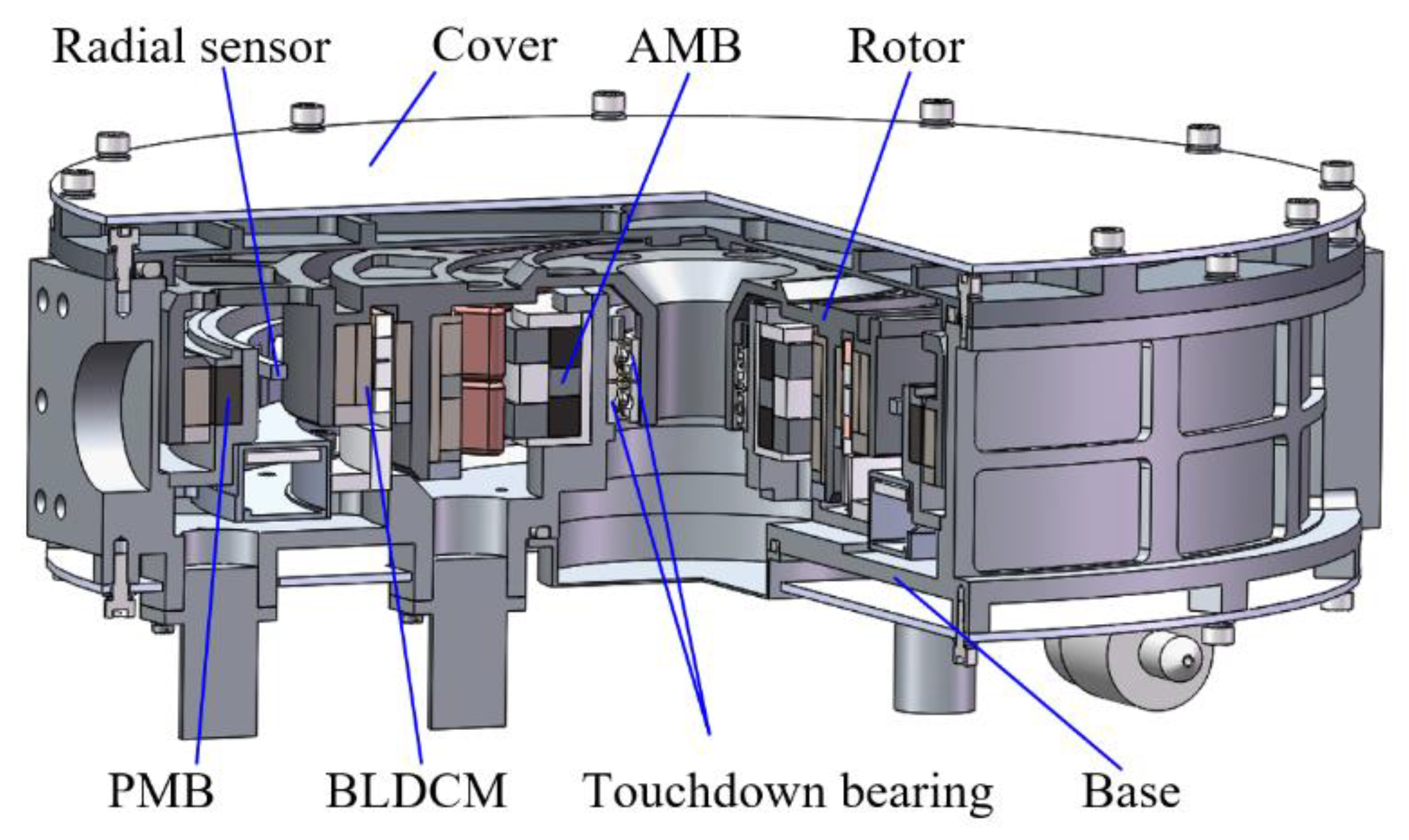
Article

Loss Estimation and Thermal Analysis of a Magnetic Levitation Reaction Flywheel with PMB and AMB for Satellite Application

1
School of Instrumentation and Optoelectronic Engineering, Beihang University, Beijing 100191, China
2
Ningbo Institute of Technology, Beihang University, Ningbo 315800, China
3
Research Institute of Frontier Science, Beihang University, Beijing 100191, China
4
Hangzhou Innovation Institute, Beihang University, Hangzhou 310051, China
*
Authors to whom correspondence should be addressed.
Energies 2022, 15(4), 1584; https://doi.org/10.3390/en15041584
Submission received: 19 December 2021 / Revised: 21 January 2022 / Accepted: 18 February 2022 / Published: 21 February 2022
(This article belongs to the Special Issue Design and Control of Flywheel Energy Storage Systems)

Abstract

:
The magnetic levitation reaction flywheel (MLRW) is a novel actuator of spacecraft attitude control because of its significant advantages, including lack of friction and active suppression of vibration. However, in a vacuum environment, the poor heat dissipation conditions make it more sensitive to various losses and rises in temperature. Therefore, increasing temperature is the key issue for components used in space. In this study, the losses of the three kinds of heat-generating areas in the MLRW, namely, the passive magnetic bearing (PMB), the active magnetic bearing (AMB) and brushless DC motor (BLDCM), were analyzed and calculated. Based on the electromagnetic field theory, the loss model of PMB was proposed. Based on the finite element method (FEM) and Bertotti model, the loss power of the AMB and the BLDCM was obtained. The calculated loss values were brought into the FEM to calculate the temperature field distribution of the MLRW system. Then, the key factors affecting the heat dissipation of the flywheel were obtained by combining thermal network analysis with the temperature field distribution. Finally, a prototype was fabricated. The maximum estimated and experimental temperatures were 34.8 °C and 36.8 °C, respectively, both at the BLDCM stator. The maximum error was 5.4%, which validates the calculated model.

1. Introduction

Reaction flywheels supported by AMBs and PMBs are very important apparatus in spacecraft attitude adjustment [1,2]. Compared with the traditional reaction flywheel supported by mechanical bearings, the MLRW has the advantages of not making contact, not requiring lubrication, and active vibration suppression [3,4,5]. In essence, it solves the problems of contact friction, lubrication, oil pollution, and vibration of the mechanical bearings, which have negative effects on the precision and life of the satellite platform. The magnetically suspended reaction flywheel is driven by a BLDCM and supported by an AMB in two radial-direction degrees-of-freedom (DOFs) and a PMB in the other three DOFs. Due to working in a high vacuum environment, there is no heat conduction by cross-ventilation. Simultaneously, there is no contact between the rotor and stator in the MLRW. Therefore, the heat is transferred between the stator and rotor of the MLRW only by the thermal radiation. Poor heat transfer efficiency causes the temperature to increase, and potentially overheating, in the MLRW system, which is the key issue for the flywheel application [6,7].
In an MLRW, the main losses are the copper and iron losses in the AMB, PMB, and BLDCM. Therefore, in order to reduce the copper losses and iron losses of the AMB, a novel structure of a radial hybrid magnetic bearing with permanent magnet (PM) bias was proposed [8]. A function of the MB power consumption was established, and was simulated and verified using the FEM [9]. Regarding the PMB, a novel radial PMB [10] and axial-radial PMB [11] were presented to increase the stability and accuracy, and decrease the losses. The loss of the flywheel system was calculated to determine the distribution of the main heat source of the system, and an equivalent thermal network model was established based on the whole mechanical topology structure [12]. Regarding the losses of the motor, a zero cogging brushless DC motor [13] and coreless stator brushless DC motor, which have high torque density, high positional stability, and low iron loss, were designed for spacecraft applications. In ref. [14], an analytical model for predicting the iron losses in high-speed shotless PM machines is presented, and was verified by 2-D FEM. Ref. [15] presents the analytical method of calculating losses of AMBs based on the reluctance network method. The proposed method of thermal analysis of the system was compared with other popular loss estimation methods. A revised method based on the Epstein Frame Method with rationale steps for deduction of the core loss in high-speed electric machines was proposed [16]. An extended survey on the evolution and the modern approaches in thermal analysis of electrical machines is presented in [17]. The 3-D FEM is also used to analyze the temperature distribution in high-speed PM electrical machines [18].
The purpose of this study was to obtain the thermal distribution of the high-speed MLRW to avoid deterioration of the electromagnetic performance of the PM, the soft magnetic alloy of the BLDCM, and the AMB under high temperature conditions. Therefore, it is necessary to study the temperature rise of MLRW systematically. The main contributions of this study are the systematic derivation of the PMB loss model, the loss calculation of the components of the MLRW, thermal analysis, and structural optimization. The copper losses of AMB and BLDCM were calculated by combining system structure analysis with Ohm’s law. The iron losses of AMB and BLDCM are composed of eddy current loss, hysteresis loss, and excess loss. The calculation method combines electromagnetic field simulation and Bertotti’s model [19]. The temperature field distribution of the MLRW system was predicted by 3-D FEM simulation. A thermal network model was set up. The structural optimization based on 3D finite element simulation and a thermal network was predicted. Finally, a prototype was fabricated to verify the calculated model.

2. Structure Scheme and Force Analysis of the MLRW

2.1. The MLRW Structure Scheme

A schematic section view of the active-passive MLRW is shown in Figure 1. The rotor driven by the BLDCM is supported by a radial AMB and an axial PMB in five DOFs. The BLDCM is proposed because of its high efficiency, long lifetime, and low power consumption. The PM biased hybrid radial magnetic bearing is used to reduce power losses while providing high precision control, achieving a greater bearing capacity and stiffness. The PMB is proposed to reduce the axial size of the shaft, reduce the power losses, and reduce the complexity of the control system in the MLRW. The reason for choosing this structure design is to reduce the coupling degree of the magnetic circuit of the PMB, AMB and BLDCM, improve the system control accuracy, and reduce the system size and power loss.

2.2. Force Analysis of the MLRW

As shown in Figure 2, the centroid coordinate system (oxyz) of the rotor is established. Since the radial AMB controls the two DOFs of the translational motions of the flywheel’s rotor, and the other three DOFs are controlled by the axial PMB, the kinetic equations of the rotor are shown below:
{ m x ¨ = f x = ( k i x i x + k x x ) m y ¨ = f y = ( k i y i y + k y y ) J z Ω ˙ = T e T d = ( e a i a + e b i b + e c i c ) / Ω T d
where m is the mass of the rotor; fx and fy are the bearing force of the AMB in the x-axis and y-axis, respectively; kix, kiy, kx and ky are the current stiffness and displacement stiffness of the AMB, respectively; Ω ˙ is the angular velocity of the MLRW; Jz is the moment of inertia of the rotor around the z-axis; Te is the torque produced by BLDCM; Td is the disturbance torque; ea, eb and ec are the induced back-EMF in the stator windings of the phases of the BLDCM; ia, ib and ic are the phase currents of the BLDCM.
The losses in the MLRW, including the stator winding loss and iron core losses of the AMB and BLDCM, and the iron core losses of the PMB, should be calculated for analysis of the thermal field and the overheating issue of the system.

3. Loss Estimation of the PMB

As there is no hysteresis loss in the PM, the excess current loss is ignored. In addition, because the other structures in the PMB are non-magnetic materials, the PMB loss is mainly due to the eddy current loss in the PM.
It can be seen from the references that the eddy current loss in the PM of the PMB is caused by the gyro effect and the PM’s non-uniform magnetization. Because the gyro effect caused by the magnetic bearing rotor radial periodic offset is controlled by the radial AMB, for the axial PMB structure used in this paper, only the eddy current loss caused by the non-uniform magnetization of the PM is considered.
The PMB structure scheme is shown in Figure 3a. Table 1 shows the design parameters for the PMB. In order to analyze the loss using the electromagnetic field theory, the polar coordinates are established. The bearing configuration schematic is shown in Figure 3b, where Σ 1 and Σ 2 represent the surfaces of the inner and outer diameters of the stator, respectively, and Σ 3 and Σ 4 represent the surfaces of the inner and outer diameters of the rotor, respectively.
Using the relationship between magnetization M and current density J, the relationship between current density J and magnetic vector potential A, the relationship between magnetic vector potential A and electric field intensity E, and the relationship between electric field intensity E and eddy current loss, we can obtain the eddy current loss of the rotor PM:
P e d d y - s t a t o r = σ i = 1 10 V R d τ S [ ( e 11 + e 21 + e 31 ) 2 + ( e 12 + e 22 + e 32 ) 2 ]
where σ is the conductivity of the PM; d τ S = R S d Φ S d z S d R S is the micro-element of the stator volume; and e 11 , e 21 , e 31 , e 12 , e 22 and e 32 represent the micro-elements of the electric field intensity generated by the rotor magnetizing current in the stator PM:
{ e 11 = μ 0 ω 4 π [ Σ 3 M i cos Φ 3 d S 3 r 3 S + Σ 3 M i sin Φ 3 ω R 3 R S sin ( Φ S Φ 3 ) r 3 S 3 d S 3 ] e 12 = μ 0 ω 4 π Σ 3 M i sin Φ 3 d S 3 r 3 S e 21 = μ 0 ω 4 π [ Σ 4 M i cos Φ 4 d S 4 r 4 S + Σ 4 M i sin Φ 4 ω R 4 R S sin ( Φ S Φ 4 ) r 4 S 3 d S 4 ] e 22 = μ 0 ω 4 π Σ 4 M i sin Φ 4 d S 4 r 4 S e 31 = μ 0 ω 4 π V R M i cos Φ R d τ R r R S 2 e 32 = μ 0 ω 4 π ( V R M i sin Φ R d τ R r R S 2 V R M i cos Φ R 2 R S R R sin ( Φ S Φ R ) r R S 4 d τ R )
where M i represents the i th harmonic amplitude of the magnetization of the rotor PM; r α S is the distance between the stator and surface Σ α ( α = 3 , 4 ) , the micro-element of the surface of the inner and outer diameters of the rotor d S α = R α d Φ α d Z α   ( α = 3 , 4 ) , the micro-element of the rotor volume d τ R = R R d Φ R d Z R d R R , and the rotor angular velocity ω = 2 π × n / 60 .
A similar expression can be written if we replace the subscripts as follows:
V S V R V R V S r 3 S r 1 R r 4 S r 2 R Σ 4 Σ 2 Σ 3 Σ 1 ω ω
Through the experiment, the axial magnetization, measured in the circumferential direction, of the PM in the PMB is shown in Figure 4.
Through the FFT transformation, the magnetization magnitude of the harmonic of the stator and rotor magnets is obtained (Figure 5).
Bringing the results into Equations (2) and (3), the eddy current loss of the rotor is Protor-eddy = 8.463 mW, and the eddy current loss of the stator is Pstator-eddy = 6.982 mW.

4. Losses Estimation of the AMB

4.1. Stator Winding Losses

The AMB’s losses consist of stator winding losses, hysteresis loss, eddy current loss, and the excess loss of the radial magnetic bearing. The scheme of AMB is shown in Figure 6a. The entity stator of the AMB is shown in Figure 6b.
The gravitational system, composed of the AMB stator and rotor, is essentially unstable. In order to overcome this nonlinear relationship between the electromagnetic force and current, in this paper, an AMB biased PM is used to linearize it. The magnetic circuit produced by the PM is shown in Figure 6c. The bias magnetic field produced by the PM provides the main bearing capacity, whereas the control current applied to the windings on the stator X+, X−, Y+, Y− is only used as a magnetic control force. The magnetic circuits produced by X+, X− stator windings with the positive control current are shown in Figure 6d,e.
We can see that, in the same direction as the control current, due to the different direction of the winding, the excitation of the magnetic field enhances the side of the air gap while weakening the other side of the air gap flux. Table 2 shows the design parameters for the AMB.
The AMB’s winding loss can be calculated by:
p C u _ c o i l = n m b R i 2 = n m b N p e A e i 2 ρ c u [ 1 + δ ( T 1 20 ) ]
where n is the number of windings, R is the winding resistance, i is the winding current, N is the number of coil winding turns, pe is the coil winding perimeter of an AMB’s pole, Ae is the effective cross-section area of coil winding, ρcu is the resistivity of the coil material (ρcu = 0.01851 Ω·mm2/m), δ is temperature coefficient of copper (δ = 0.004/°C), T1 is the test temperature. Because of the PM biased AMB, no biased current exists in the windings. In the MLRW, winding losses and currents of the AMB are calculated by Equation (4) and shown in Table 3, with a rotation speed of 5000 r/min and extreme vacuum of 1.8 × 10⁻⁷ Pa. The total winding loss of the AMBs is 0.074 W at 20 °C. The winding loss is affected by temperature, and the resultant curves are shown in Figure 7.

4.2. Iron Loss Estimation of AMB

In this study, the iron losses in the AMB can be divided into the eddy current loss, the hysteresis loss, and the excess loss. All of these are affected by the core material, the magnetic field changes in frequency, the magnetic flux density, and the volume of the core. The iron losses of the AMB occur in the stator and rotor.
The stator core and rotor core use lamination material 1J50, which is used to reduce losses in the eddy currents. The eddy current loss may appear in the case of a shaft position fluctuation. The eddy current loss can be estimated as:
P R _ e d d y = k c f R 2 B R 2 V R
where kc is the coefficient of eddy current loss; fR is the operating frequency of the magnetic field changes in the frequency of the AMB, which is twice as large as the mechanical frequency because two flux density periods are contained in a geometric period of the shaft; BR is the maximum flux density; VR is the affected volume.
The hysteresis loss can be calculated according to the analytical equation:
P R _ h y s = k h f R B m α V R
where kh is the factor of hysteresis loss and α is the Steinmetz constant.
The excess loss can be expressed as:
P R _ e x = k e f R 1.5 B R 1.5 V R
where ke is the coefficient of the anomalous eddy current loss.
The combined estimation equation for the iron core losses can be also presented in the form:
P R _ c o r e = ( k h f R B R α + k c f R 2 B R 2 + k e f R 1.5 B R 1.5 ) V R
The iron loss depends on the loss factor of the iron core material, the magnetic field changes in the frequency, the flux density amplitude, and the volume of the core. In this study, the AMB was made of a silicon steel sheet with a thickness of 0.2 mm. According to the loss curves of the silicon steel sheets with a sinusoid supply (Figure 8), the loss factors and Steinmetz constant calculated by the direct fitting computed method are shown in Table 4.
The main parameters and loss calculation results are shown in Table 5, which shows that the total loss is 0.786 W, and the percentages of different loss types are shown in Table 6. The eddy current and hysteresis losses are the major losses, whereas the excess loss is the smallest loss (0.13% of the total iron loss), and can be ignored in the iron loss. The hysteresis loss, classical eddy current loss, and excess eddy current loss versus magnetic magnitude, while the AMB is working with a rotation speed of 5000 r/min, are shown in Figure 9.
In addition to the stator and rotor core of the AMB, the iron loss also exists in the magnet ring, the PM, and the return ring. As solid materials are used in the above elements, the iron loss calculation formula is slightly different from that in Equation (8). Ignoring the excess loss, the iron loss can be expressed as:
P S _ i r o n = P S _ h + P S _ e = ( k S _ h + k S _ e ) σ S δ S 2 f S 2 B S 2 V S
where kS_h is the hysteresis loss factor, kS_e is the eddy current loss factor, σS is the conductivity, δS is the thickness, BS is the maximum flux density, fS is the operating frequency of the AMB, VS is the effective volume. The iron cobalt vanadium soft magnetic alloy was adopted in this prototype. The main parameters and loss calculation results are shown in Table 7.

5. Loss Estimation of the BLDCM

Space applications generally require low-power reaction wheel systems. Thus, a three-phase BLDCM with ironless and slotless stator was used in the MLRW for driving the rotor to rotate at a high speed [20,21]. The structure and parameters of the BLDCM are shown in Figure 10 and Table 8, respectively. The stator winding coil and Hall sensor are fixed on the stator frame constructed of polyimide. The rotor consists of the PM poles comprising the SmCo magnet, outer rotor core, and inner rotor core made of the 1J50 material (perm alloy with 50% nickel). The range of the speed is from −5000 r/min to 5000 r/min, which can output torques in both directions. Therefore, the loss type in the BLDCM consists of the iron core loss from the rotor and the coil copper loss from the stator.

5.1. Stator Winding Losses

Because the current passes through the windings and the polyimide stator frame, the stator loss of the BLDCM consists mainly of the copper loss. Considering the influence of the temperature on the armature windings, the coil copper loss can be expressed as:
P c o i l M = n M R c i c 2 = n M N c p c A c ρ c u [ 1 + δ ( T c 20 ) ] i c 2
where nM is number of the phases and Tc is the test temperature. Rc, ic, Nc, pc, Ac, ρcu and δ represent the same parameters as in Equation (4) for the BLDCM. The estimated results of the coil losses have a positive correlation with the temperature of the BLDCM, as shown in Figure 11. At room temperature, the total copper losses are 2.91 W.

5.2. Rotor Losses Estimation

In the BLDCM, the rotor loss consists of the inner rotor core loss, outer rotor core loss, and PM loss. Similarly to the AMB, the iron losses are separated into the hysteresis loss, eddy current loss, and excess loss. PM losses are caused by the induced eddy current.
The iron core is made up of thin laminations in order to reduce iron core loss. The iron core loss depends on the loss factor of iron core material, flux density amplitude, and magnetic field changes in frequency. From refs. [22,23], the iron loss of the 1J50 material consists of the eddy current loss, hysteresis loss, and excess loss, and can be calculated as:
P M = P h M + P c M + P e M { P h M = K h f k = 0 k ( B k max α + B k min α ) V M P c M = K c f 2 k = 0 k 2 ( B k max 2 + B k min 2 ) V M P e M = K e ( 2 π ) 3 2 1 T 0 T ( | d B r ( t ) d t | 1.5 + | d B θ ( t ) d t | 1.5 ) d t V M
where Kh, Kc, Ke and α are shown in Table 4 for the same material; Bkmax and Bkmin are the maximum and minimum values of the elliptical harmonic of each order, respectively [24]; Br and Bθ are the radial and circumferential components, respectively. f is the operating frequency of the magnetic field, T = 60/(p ×  n) = 0.0015 s, and Vpm is the effective volume.

5.2.1. Loss Estimation of the Inner Rotor Core

When the MLRW works with the rotation speed of 5000 r/min, the maximum and the minimum FFT values of the harmonics in the inner rotor core are calculated (Figure 12).
According to Equation (11), since the amplitudes of the harmonics over an order of 17 are smaller and negligible, only the maximum 17-order harmonic magnetic flux density is considered. It can be calculated that the hysteresis loss and eddy current loss in the inner rotor core are 0.472 and 0.00168 W, respectively.
{ P i n _ h M = K h f M k = 0 17 k ( B k max α + B k min α ) V i n M P i n _ c M = K c f M 2 k = 0 17 k 2 ( B k max 2 + B k min 2 ) V i n M
where fM = p M × n m / 60 Hz, p M is the pole pair number of the BLDCM, n M is the rated speed, V i n M is the effective volume of the inner rotor core.
The first derivative of the radial and axial flux density in the inner rotor core is calculated in Figure 13a,b, respectively.
According to the excess loss formula given in Equation (11) and the computed data in Figure 13a,b, it can be calculated that the excess loss in the inner rotor core is 0.0009 W.
P i n _ e M = K e ( 2 π ) 3 2 1 T 0 T ( | d B r ( t ) d t | 1.5 + | d B θ ( t ) d t | 1.5 ) d t V i n M

5.2.2. Loss Estimation of the Outer Rotor Core

Similarly, the maximum and the minimum FFT values of the harmonics in the outer rotor core are calculated (Figure 14).
It can be calculated that the hysteresis loss and eddy current loss in the outer rotor core are 0.626 and 0.00364 W, respectively.
{ P o u _ h M = K h f m k = 0 17 k ( B k max α + B k min α ) V o u M P o u _ c M = K c f m 2 k = 0 17 k 2 ( B k max 2 + B k min 2 ) V o u M
where V o u M is the effective volume of the outer rotor core.
The first derivative of the radial and axial flux density in the outer rotor core is calculated in Figure 15a,b, respectively.
According to the excess loss formula given in Equation (11) and the computed data in Figure 15a,b, it can be calculated that the excess loss in the inner rotor core is 0.00207 W.
P o u _ e M = K e ( 2 π ) 3 2 1 T 0 T ( | d B r ( t ) d t | 1.5 + | d B θ ( t ) d t | 1.5 ) d t V o u M

5.2.3. Loss Estimation of the PM

The calculation results of the harmonic amplitude in the PM of the BLDCM at the rated speed are shown in Figure 16.
There is no hysteresis loss in the PM, and the eddy current loss produced by the harmonic flux density can be expressed as:
P i e = 1 T 0 T 0 d p 2 0 L τ i 2 τ i 2 J i 2 ( x , t ) σ i d x d y d z d t
Since the other higher harmonics magnetic flux density are small and negligible, only the first 17 orders of the harmonics are calculated in the eddy current loss.
P P M M = n = 1 17 α P M σ P M L P M d P M τ n 3 B n 2 ω e n 2 16 ( δ n 3 τ n sinh δ n τ n sin δ n τ n c o s h δ n τ n cos δ n τ n )
where τn is the polar distance of the space harmonics ( τ n = π D r 2 n p , Dr is the inner diameter of the PM), ωen is the electrical angular velocity, σ P M = 1.17 × 10⁶ S/m is the conductivity of the PM, α P M = 0.67 is the pole-arc coefficient. Substituting parameters and values into Equation (17), the result of the eddy current loss of the PM of the rotor is P P M M = 3.42 W.

6. Thermal Field Analysis and Measurement for the Prototype of MLRW

6.1. Calculation for Heat Generation Rate

The various losses in the MLRW can eventually be converted to a temperature increase. As mentioned above, these losses consist of the copper losses and iron core losses in the AMB and the BLDCM, and they are regarded in terms of the heat generation rate per unit volume. The models of energy transfer, including the heat conduction and thermal radiation, play a major role in cooling MLRW when working in a highly vacuum state.
The heat generation rates of the copper loss of the coils in the MBs and the BLDCM are calculated by Equation (18) and the results are shown in Table 9. The total copper loss of the MLRW is 2.98 W.
q l o s s = P l o s s V E V
The heat generation rates of the iron core loss in the MBs and the BLDCM are calculated by Equation (18) and shown in Table 10. The loss percentages of the loss types and the different parts are shown in Table 11 and Table 12, respectively. The total loss, including the copper loss and the iron core loss, is 8.75 W. The total iron core loss of the MLRW is 5.77 W. The estimated results show the BLDCM loss is the main loss, accounting for 84.98% of the total loss in the MLRW.

6.2. Convection Heat Transfer Coefficient

The thermal analysis of the system conforms to the law of conservation of energy, namely, for any closed system:
Q W = Δ U + Δ K E + Δ P E
where Q is the heat in the system; W is the external work; Δ U is the change in the internal energy of the system; Δ K E is the kinetic energy of the system; Δ P E is the potential energy of the system. For most engineering heat conduction problems, Δ K E = Δ P E = 0 . For the flywheel thermal analysis studied in this paper, when the flywheel is working in a stable situation, the heat generated by the flywheel is equal to the heat dissipated into the space; that is, Q W = 0 .
Because of the high-vacuum working situation, the effect of heat convection caused by air can be ignored. The heat transfer formula of the heat conduction due to the contact between different temperature objects is:
Q i t = K A ( T h o t T c o l d ) / d
where Q i is the heat transferred in time t ; K is the heat transfer coefficient; A is the effective area between the two contact objects; T is the temperature of the object; and d is the distance between the two planes.
The heat transfer formula of heat radiation is:
Φ 1 , 2 = σ b ( T 1 4 T 2 4 ) 1 ε 1 ε 1 A 1 + 1 A 1 X 1 , 2 + 1 ε 2 ε 2 A 2
where Φ 1 , 2 is the heat flux between surfaces 1 and 2; σ b = 5.67 × 10 8   W / ( m 2 × K 4 ) is the radiation constant for the blackbody; ε 1 , ε 2 are the emissivities of the radiation of surfaces 1 and 2; A1, A2 are the effective areas of radiating faces 1 and 2, respectively; T1, T2 are the surface temperatures of the radiation surfaces 1 and 2, respectively; X 1 , 2 is the coefficient between the radiating surfaces 1 and 2 (representing the ratio of the total radiation emitted by surface 2 to the amount of the radiation absorbed by surface 1).

6.3. Thermal Field Analysis of the MLRW

The thermal behavior of the MLRW depends on its cooling capability and losses in the system. The 3-D FEM of the MLRW was built based on the ANSYS software. Its mesh is shown as Figure 17a, and the total number of nodes was 426,034. The ambient temperature was set to 20 °C. Conduction and radiation are the heat transfer modes for the internal cooling of MLRW. The heat convection can be ignored on account of the high-vacuum environment. Due to the tight assembly between the components, the heat transfer mode is mainly heat conduction. Although the rotor is supported by magnetic levitation in the vacuum environment, the cooling of the rotor is only by means of thermal radiation. Based on steady-state thermal analysis, thermal parameters such as thermal conductivity, specific heat capacity, emissivity, and loss-load per unit volume of each component are assigned to the FEM of thermal distribution. The estimated temperature result is shown in Figure 17b. (In order to facilitate observation, a portion of the lower temperature components are hidden). The estimated maximum temperature is 54.2 °C, which is located at the BLDCM stator.

6.4. Thermal Optimization Design Based on Thermal Network Model

When the heat dissipation method and the heat transfer mode of the system are analyzed by the thermal network method, the components of the MLRW are equivalent to the individual node units. Each node contains the size of its own heat generation value and various heat-related parameters, such as the thermal conductivity and specific heat capacity. The heat transfer path between the components is expressed by the thermal conductivity or thermal resistance between the node units. The equivalent node unit and heat dissipation path is shown in Figure 18.
Then, the heat transfer relationship of each node unit can be expressed as the equivalent thermal network model, as shown in Figure 19.
The heat change formula on any node is:
c i d T i d t = j E i , j ( T j 4 T i 4 ) + j D i , j ( T j T i ) + q i
where c i represents the specific heat capacity of the node i; T i represents the temperature of node i; q i is the amount of heat generated internally by the corresponding node i per unit time; E i , j is the thermal radiation coefficient between node i and node j; D i , j is the thermal conductivity between node i and node j.
According to the Equations (20) and (21), the thermal conductance formula caused by the radiation and conductivity is:
{ E i , j = σ b 1 ε i ε i A i + 1 A i X i , j + 1 ε j ε j A j D i , j = λ i A i , j δ i , j
where δ i , j is the distance of the thermal conductivity and λ i is the conductivity coefficient of node i.
According to the thermal field diagram of the MLRW shown in Figure 17b, the temperature of the PM and stator windings of the BLDCM correspond to node i7 and i10 in the equivalent thermal network model. The thermal parameters, such as the thermal radiation coefficient, thermal conductivity, and heat rate of different components in the MLRW for the thermal distribution, are based on the steady-state thermal analysis [25,26]. Therefore, the optimization target is to reduce the temperature of node i7 and i10. Then, in the thermal network equations of the whole system, there are:
{ E 7 , 8 ( T 8 4 T 7 4 ) + E 7 , 10 ( T 10 4 T 7 4 ) + E 7 , 13 ( T 13 4 T 7 4 ) + D 7 , 14 ( T 14 T 7 ) + q 7 = 0 E 7 , 10 ( T 10 4 T 7 4 ) + D 9 , 10 ( T 10 T 9 ) + D 10 , 13 ( T 13 T 10 ) + q 10 = 0
By calculation and comparison of the values of the thermal conductance of each heat transfer path, it was found that the thermal conductance of node i14 is too small, which affects the heat dissipation efficiency of nodes i7 and i10. Thus, the polyimide of the fixed BLDCM stator windings was replaced by 1060 alloy, which has better thermal conductivity and hear emissivity. The results of the 3-D FEM verification are shown in Figure 20, and the maximum temperature located at the BLDCM stator is reduced from 54.2 to 34.8 °C.

7. Experimental Test

The prototype of the MLRW with the rated speed of 5000 r/min was manufactured in this study (Figure 21a). The MLRW was measured to confirm the loss estimation and the thermal field analysis. Four temperature measurement points were selected in the prototype, as shown in Figure 21b, where the thermistors were located at the PMB stator, base, BLDCM stator, and AMB stator.
The temperature rise curve when the MLRW reaches the rated rotation speed of 5000 r/min is shown in Figure 21c. It is shown that, when the MLRW thermal distribution is stable, the highest temperature is located at the end of the BLDCM stator windings, and the value is 36.8 °C. The maximum temperatures of the AMB stator and PMB stator are 30.1 and 24.5 °C respectively. The maximum temperature increase in the MLRW satisfies the safety margin of the magnetic and metal materials. The maximum temperature of the base is 24.5 °C. The errors in the calculated and measured values are shown in Table 13, with the maximum error of less than 10%. Thus, the experimental results verified the accuracy of the MLRW loss estimation and thermal field analysis.

8. Conclusions

In this article, the temperature increase due to the copper and iron losses in a MLRW was calculated. The copper and iron core losses in the PMB, AMB, and BLDCM were all predicted by their analytical equations. The thermal field of the prototype was analyzed by the 3-D FEM based on the loss values and the heat generation rates. The estimated maximum temperature was found to be located at the BLDCM stator, and the temperature was 34.8 °C. A prototype was fabricated, and the maximum measured temperature, also located at the BLDCM stator, was 36.8 °C. The maximum error between the calculated and measured temperatures was 5.4%, which verifies the loss estimation model and the thermal field analysis and optimization.

Author Contributions

Methodology and Writing—original draft, Z.H.; Project administration, T.W.; Supervision, X.L.; Validation, Y.S. All authors have read and agreed to the published version of the manuscript.

Funding

This work was supported by the National Natural Science Foundation of China (Grant Nos. 51925501, 82027802, 62073010 and 61773038), and in part by the supported by Ningbo Natural Science Foundation (No. 2021J011).

Institutional Review Board Statement

Not applicable.

Informed Consent Statement

Not applicable.

Data Availability Statement

Not applicable.

Conflicts of Interest

The authors declare no conflict of interest.

References

  1. Zhang, J.; Yuan, L.; Chen, S.L.; Liang, Y.; Yang, G. A survey on design of reaction spheres and associated speed and orientation measurement technologies. ISA Trans. 2019, 99, 417–431. [Google Scholar] [CrossRef] [PubMed]
  2. Tang, J.; Fang, J.; Wen, W. Superconducting Magnetic Bearings and Active Magnetic Bearings in Attitude Control and Energy Storage Flywheel for Spacecraft. IEEE Trans. Appl. Supercond. 2012, 22, 5702109. [Google Scholar] [CrossRef]
  3. Zhang, W.; Zhu, H.; Yang, H.; Chen, T. Experimental Analysis and Full Prediction Model of a 5-DOF Motorized Spindle. Energies 2017, 10, 75. [Google Scholar] [CrossRef] [Green Version]
  4. Mao, C.; Zhu, C. Vibration Control for Active Magnetic Bearing Rotor System of High-Speed Flywheel Energy Storage System in a Wide Range of Speed. In Proceedings of the 2016 IEEE Vehicle Power and Propulsion Conference (VPPC), Hangzhou, China, 17–20 October 2016; pp. 1–6. [Google Scholar]
  5. Zhao, Y.; Lu, F.; Fan, C.; Yang, J. A Novel Axial-Flux Dual-Stator Toothless Permanent Magnet Machine for Flywheel Energy Storage. Symmetry 2022, 14, 61. [Google Scholar] [CrossRef]
  6. Yu, Y.; Zhang, W.; Sun, Y.; Xu, P. Basic Characteristics and Design of a Novel Hybrid Magnetic Bearing for Wind Turbines. Energies 2016, 9, 905. [Google Scholar] [CrossRef] [Green Version]
  7. Ji, W.; Ni, F.; Gao, D.; Luo, S.; Lv, Q.; Lv, D. Electromagnetic Design of High-Power and High-Speed Permanent Magnet Synchronous Motor Considering Loss Characteristics. Energies 2021, 14, 3622. [Google Scholar] [CrossRef]
  8. Sun, J.; Fang, J. A novel structure of permanent-magnet-biased radial hybrid magnetic bearing. J. Magn. Magn. Mater. 2011, 323, 202–208. [Google Scholar]
  9. Wang, H.; Wu, J.F.; Li, Y.; Wu, Y.H. Thermal design of attitude control flywheel system for small satellites. Opt. Precis. Eng. 2015, 23, 2265. [Google Scholar] [CrossRef]
  10. Tir, M.A.; Mirimani, S.M.; Marignetti, F. A novel structure of passive magnetic bearing with axial magnetization. In Proceedings of the 5th Annual International Power Electronics, Drive Systems and Technologies Conference (PEDSTC 2014), Tehran, Iran, 5–6 February 2014; pp. 311–316. [Google Scholar]
  11. Tănase, N.; Morega, A.M.; Nedelcu, A.; Ilie, C. Radial-axial passive magnetic bearing system—Numerical simulation aided design solutions. In Proceedings of the 2015 9th International Symposium on Advanced Topics in Electrical Engineering (ATEE), Bucharest, Romania, 7–9 May 2015; pp. 566–572. [Google Scholar]
  12. Liu, Q.; Zhao, M.S.; Han, B.C.; Fan, Y.H.; Sun, J.J.; Zheng, S.Q. Energy optimization and experimental for a permanent magnet-biased redial magnetic bearing. Opt. Precis. Eng. 2019, 27, 2420–2428. [Google Scholar]
  13. Achari, V.; Jagathy, R.; Madhu, G.; Bindu, G.R. Design and analysis of zero cogging Brushless DC motor for spacecraft applications. In Proceedings of the 2010 ECTI International Confernce on Electrical Engineering/Electronics, Computer, Telecommunications and Information Technology, Chaing Mai, Thailand, 19–21 May 2010; pp. 254–258. [Google Scholar]
  14. Chebak, A.; Viarouge, P.; Cros, J. Analytical Computation of the Full Load Magnetic Losses in the Soft Magnetic Composite Stator of High-Speed Slotless Permanent Magnet Machines. IEEE Trans. Magn. 2009, 45, 952–955. [Google Scholar] [CrossRef]
  15. Romanenko, A.; Smirnov, R.; Jastrzebski, P.; Pyrhönen, O. Losses estimation and modelling in active magnetic bearings. In Proceedings of the 2014 16th European Conference on Power Electronics and Applications, Lappeenranta, Finland, 26–28 August 2014; pp. 1–8. [Google Scholar]
  16. Su, W.M.; Mao, S.H.; Wang, P.J. Core losses estimation in design of high speed electric machines. In Proceedings of the 2016 Progress in Electromagnetic Research Symposium (PIERS), Shanghai, China, 8 August–11 September 2016; pp. 320–323. [Google Scholar]
  17. Boglietti, A.; Cavagnino, A.; Staton, D.; Shanel, M.; Mueller, M.; Mejuto, C. Evolution and Modern Approaches for Thermal Analysis of Electrical Machines. IEEE Trans. Ind. Electron. 2009, 56, 871–882. [Google Scholar] [CrossRef] [Green Version]
  18. Huang, Z.; Fang, J.; Liu, X.; Han, B. Loss Calculation and Thermal Analysis of Rotors Supported by Active Magnetic Bearings for High-Speed Permanent-Magnet Electrical Machines. IEEE Trans. Ind. Electron. 2016, 63, 2027–2035. [Google Scholar] [CrossRef]
  19. Bertotti, G. General properties of power losses in soft ferromagnetic materials. IEEE Trans. Magn. 1988, 24, 621–630. [Google Scholar] [CrossRef]
  20. Fang, J.; Li, W.; Li, H. Self-Compensation of the Commutation Angle Based on DC-Link Current for High-Speed Brushless DC Motors with Low Inductance. IEEE Trans. Power Electron. 2014, 29, 428–439. [Google Scholar] [CrossRef]
  21. Han, B.; Zheng, S.; Wang, Z.; Le, Y. Design, Modeling, Fabrication, Test of A Large Scale Single-Gimbal Magnetically Suspended Control Moment Gyro. IEEE Trans. Ind. Electron. 2015, 62, 7424–7435. [Google Scholar] [CrossRef]
  22. Binesti, D.; Ducreux, J.P. Core Losses and Efficiency of Electrical Motors Using New Magnetic Materials. IEEE Trans. Magn. 1996, 32, 4887–4889. [Google Scholar] [CrossRef]
  23. Roshen, W. Iron Loss Model for Permanent Magnet Synchronous Motors. IEEE Trans. Magn. 2007, 43, 3428–3434. [Google Scholar] [CrossRef]
  24. Kong, X.; Wang, F.; Xu, Y.; Xing, J. Analysis and calculation of iron losses of high-speed permanent magnet machines. Electr. Mach. Control. 2010, 14, 26–30. [Google Scholar]
  25. Zhang, S.; Han, B.; Hong, L.; Fang, J. Thermal and structural coupling analysis of magnetically suspended flywheel rotor. In Proceedings of the Sixth International Symposium on Instrumentation and Control Technology, Beijing, China, 13–15 October 2006. [Google Scholar]
  26. Zhai, L.; Sun, J.; Ma, X.; Han, W.; Luo, X. Thermal–structure coupling analysis and multi-objective optimization of motor rotor in MSPMSM. Chin. J. Aeronaut. 2019, 32, 1733–1747. [Google Scholar] [CrossRef]
Figure 1. Structure of the MLRW.
Energies 15 01584 g001
Figure 2. Force analysis and coordinate system of the MLRW.
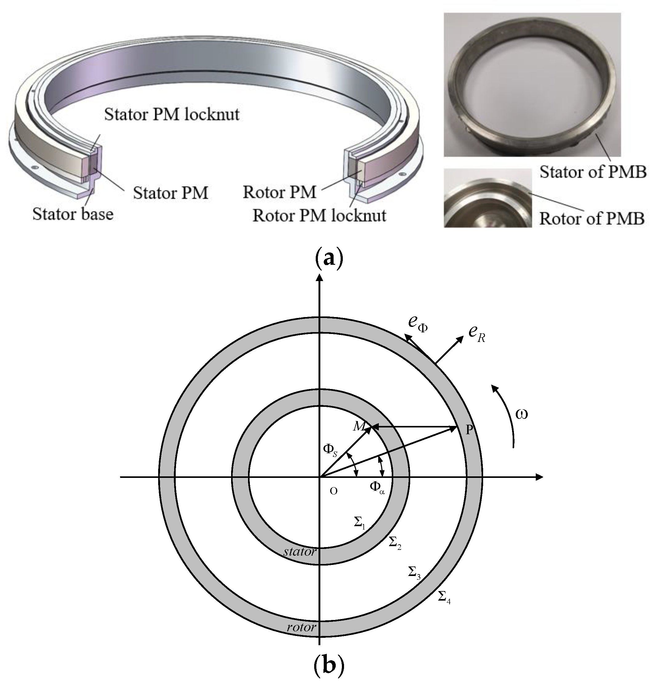
Energies 15 01584 g002
Figure 3. PMB scheme. (a) The structure of the PMB. (b) Bearing configuration schematic.
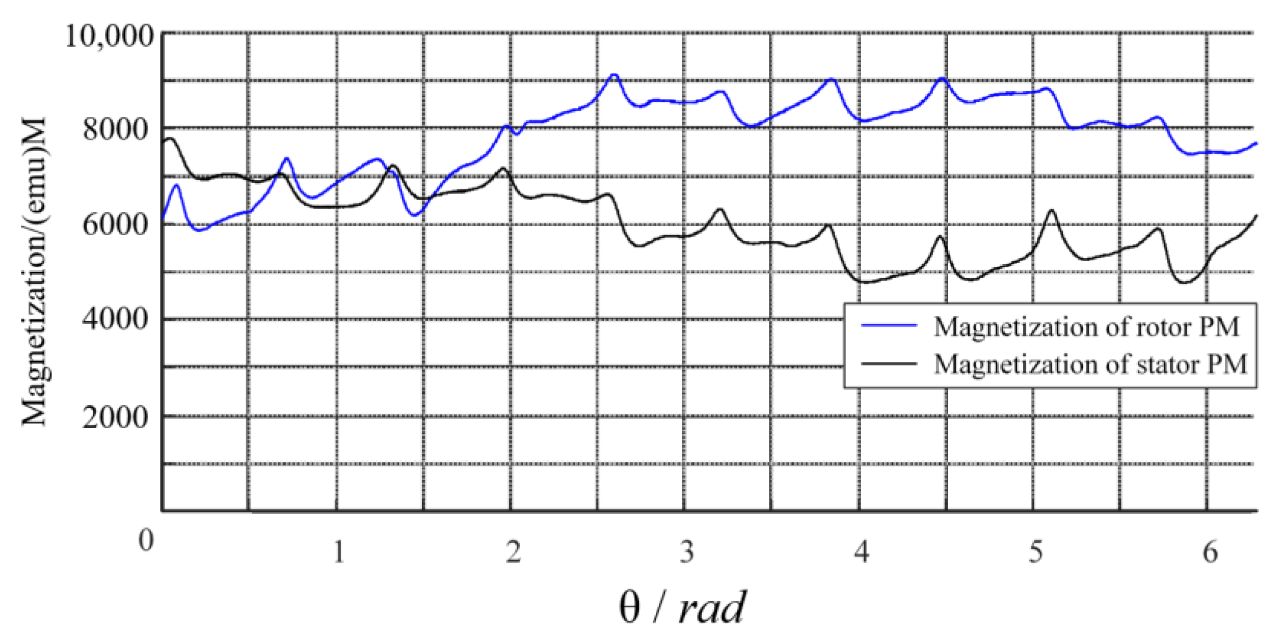
Energies 15 01584 g003
Figure 4. Axial magnetization of the PM in the PMB.
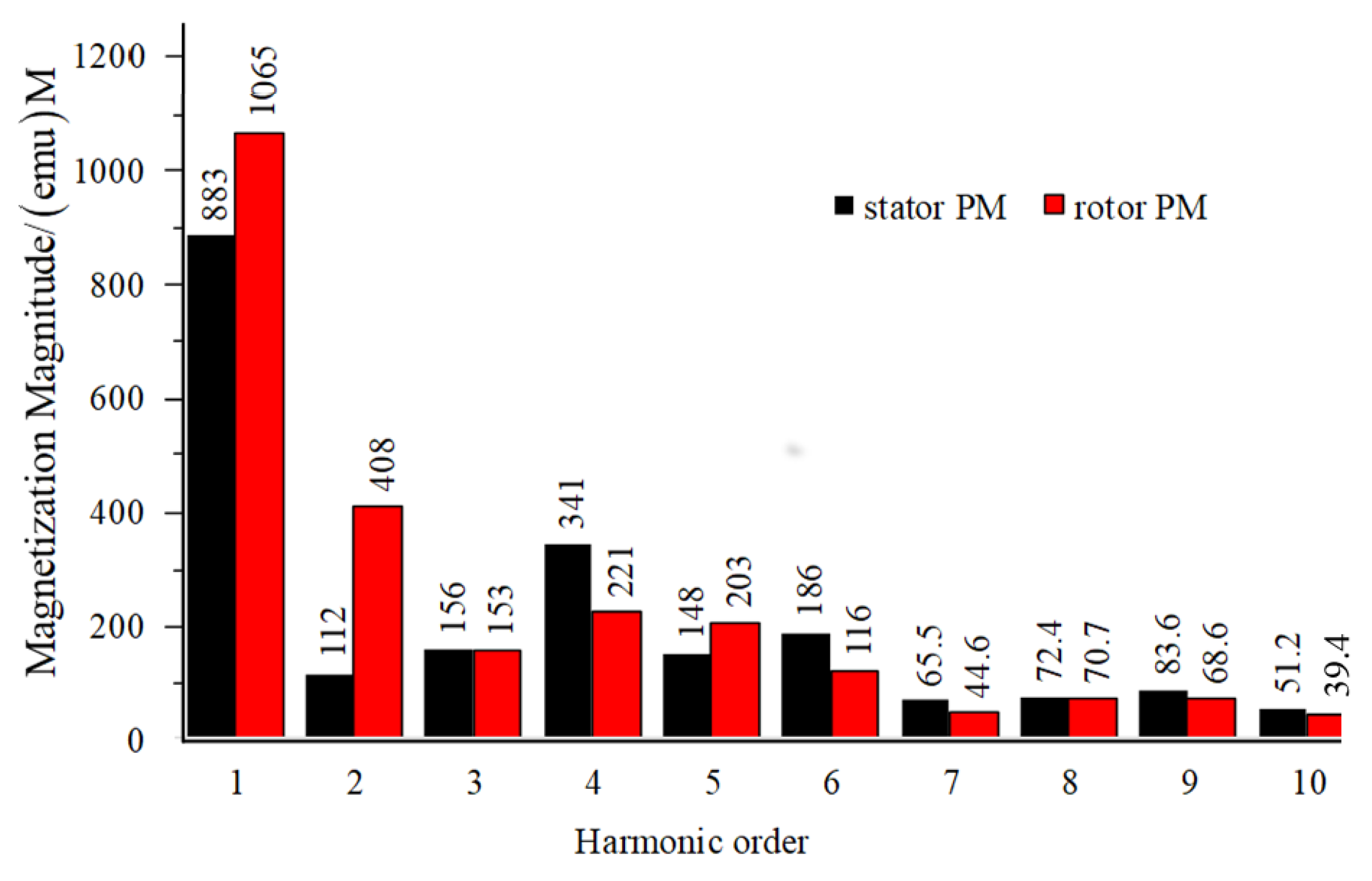
Energies 15 01584 g004
Figure 5. The magnetization magnitude of the harmonic of the PMB.
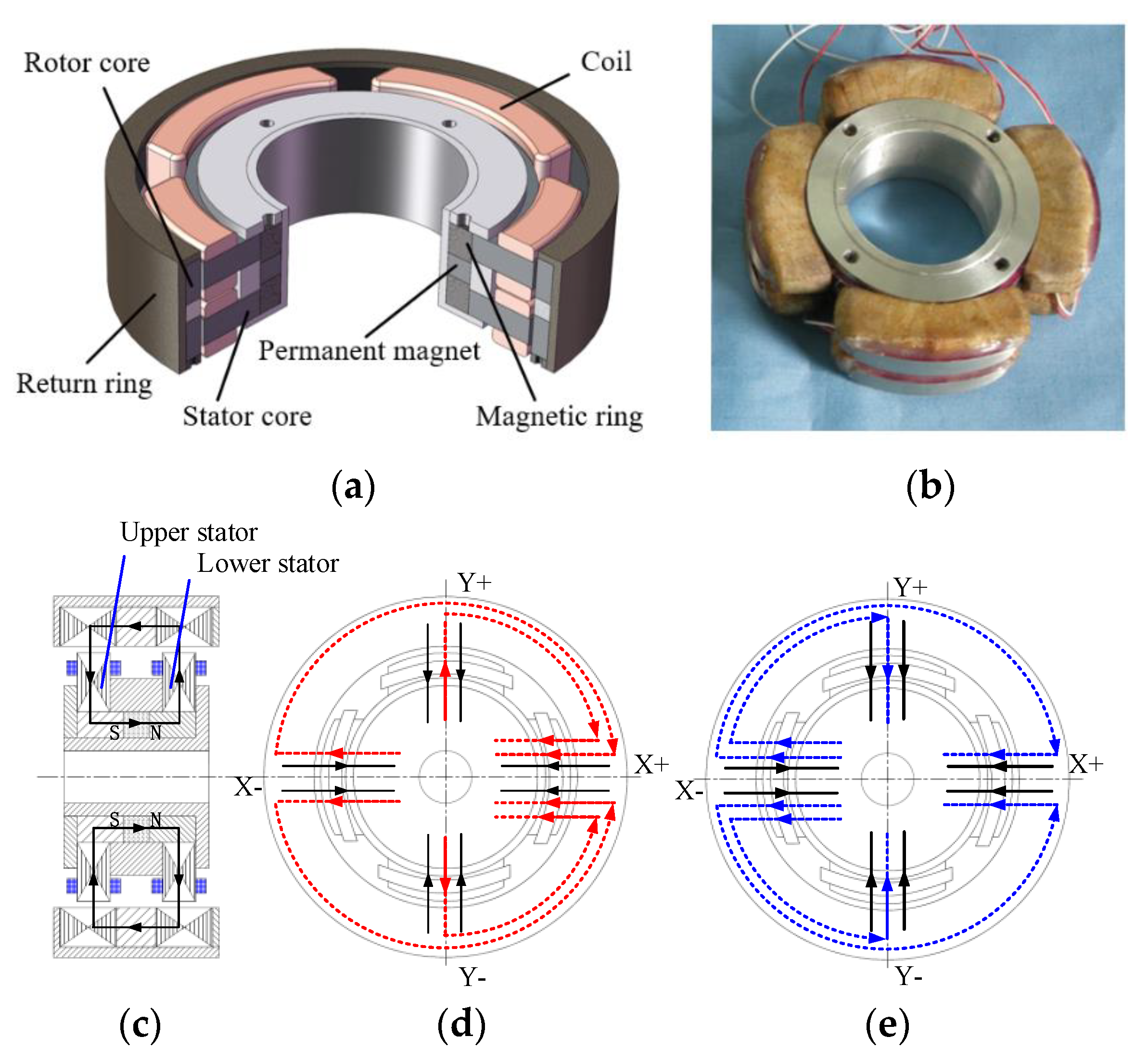
Energies 15 01584 g005
Figure 6. Structure of the AMB. (a) Scheme of the AMB structure. (b) The stator of the AMB. (c) Scheme of the PM magnetic circuit. (d) Scheme of the magnetic circuit of X+ winding with positive excitation current (upper stator). (e) Scheme of the magnetic circuit of X− winding with positive excitation current (upper stator).
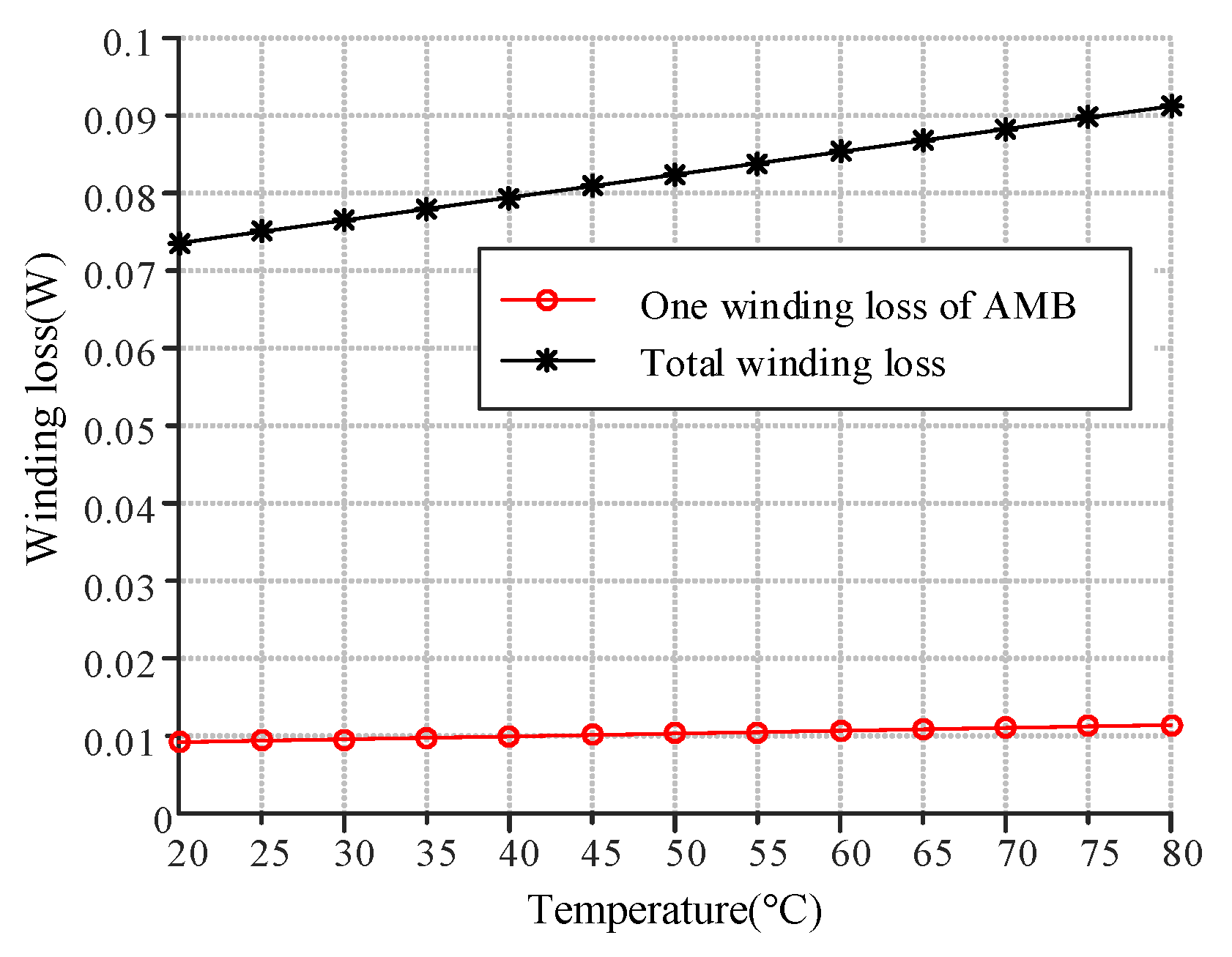
Energies 15 01584 g006
Figure 7. Winding loss versus temperature for the AMB.
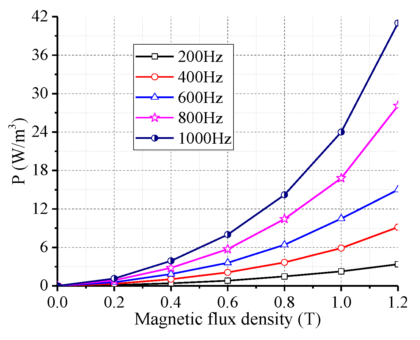
Energies 15 01584 g007
Figure 8. Loss curves of the silicon sheet with a sinusoid supply.
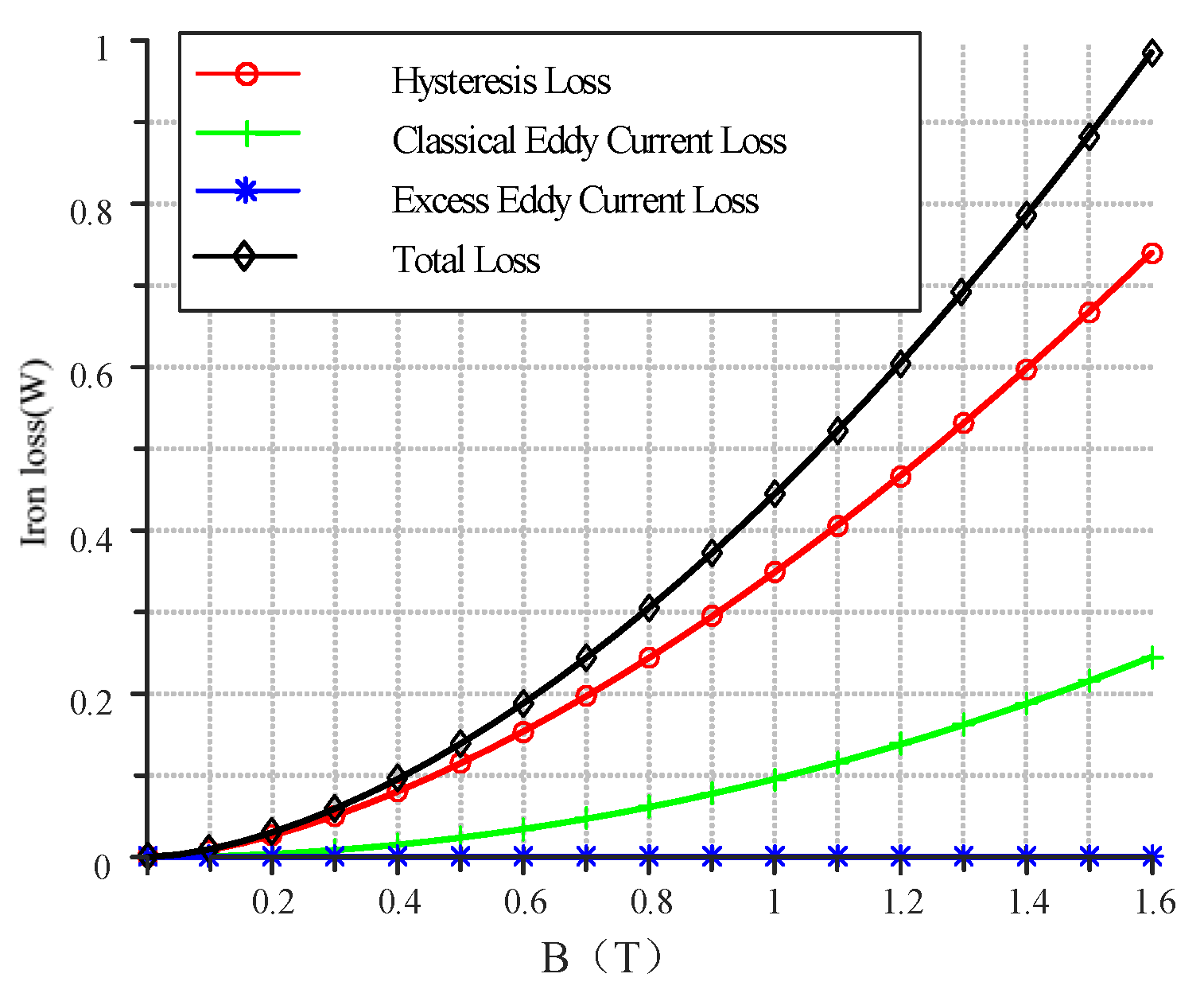
Energies 15 01584 g008
Figure 9. Hysteresis loss curve, classical eddy current loss curve, and excess eddy current loss curve in the AMB versus magnetic magnitude.
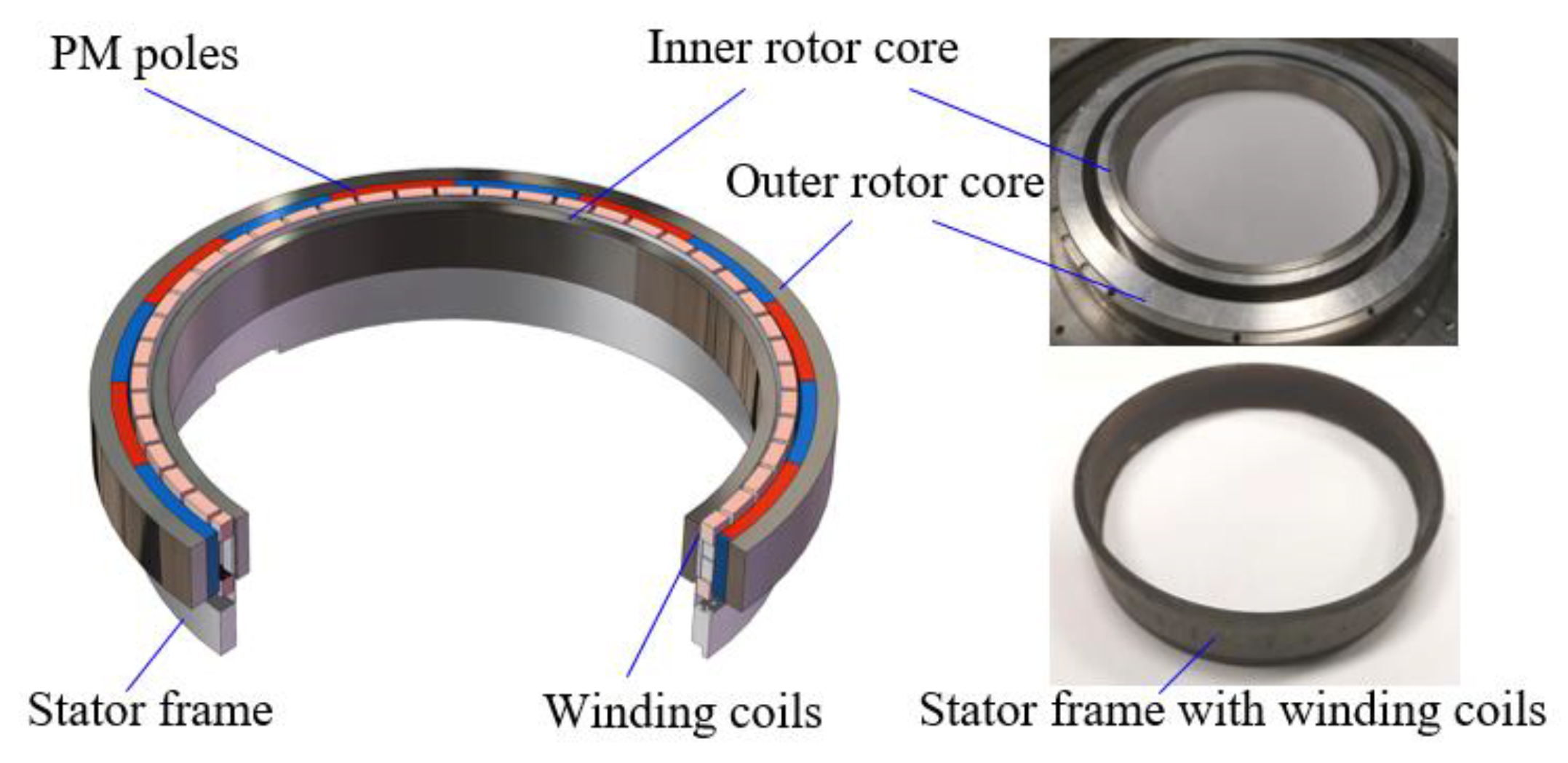
Energies 15 01584 g009
Figure 10. Structure of the BLDCM.
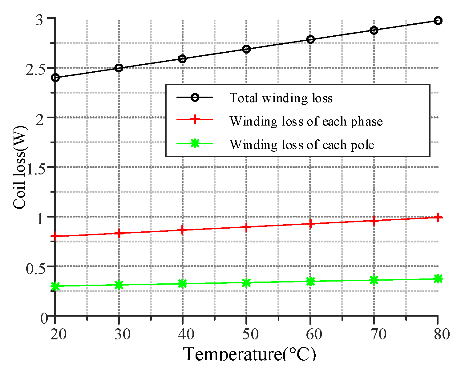
Energies 15 01584 g010
Figure 11. Winding loss of the BLDCM affected by temperature.
Energies 15 01584 g011
Figure 12. The maximum and minimum FFT values of the harmonics in the inner rotor core.
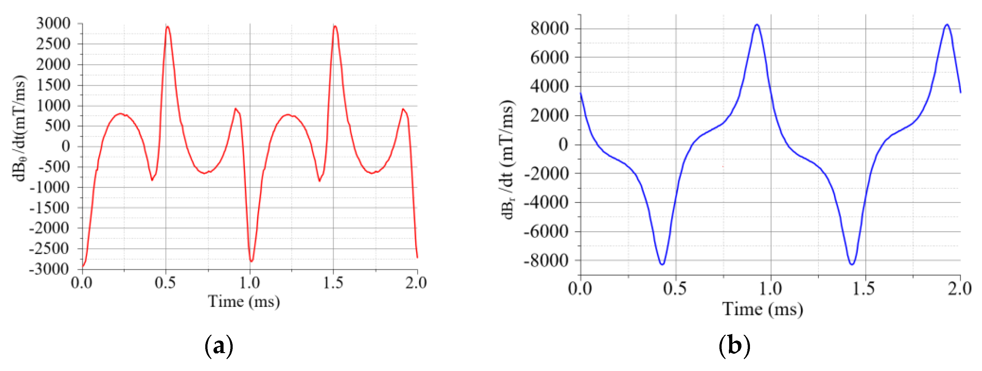
Energies 15 01584 g012
Figure 13. The first derivative of the radial and axial flux density in the inner rotor core. (a) Radial. (b) Axial.
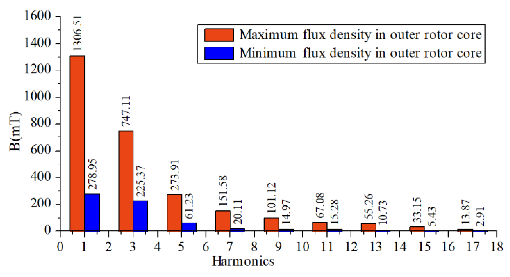
Energies 15 01584 g013
Figure 14. The maximum and minimum FFT values of the harmonics in the outer rotor core.
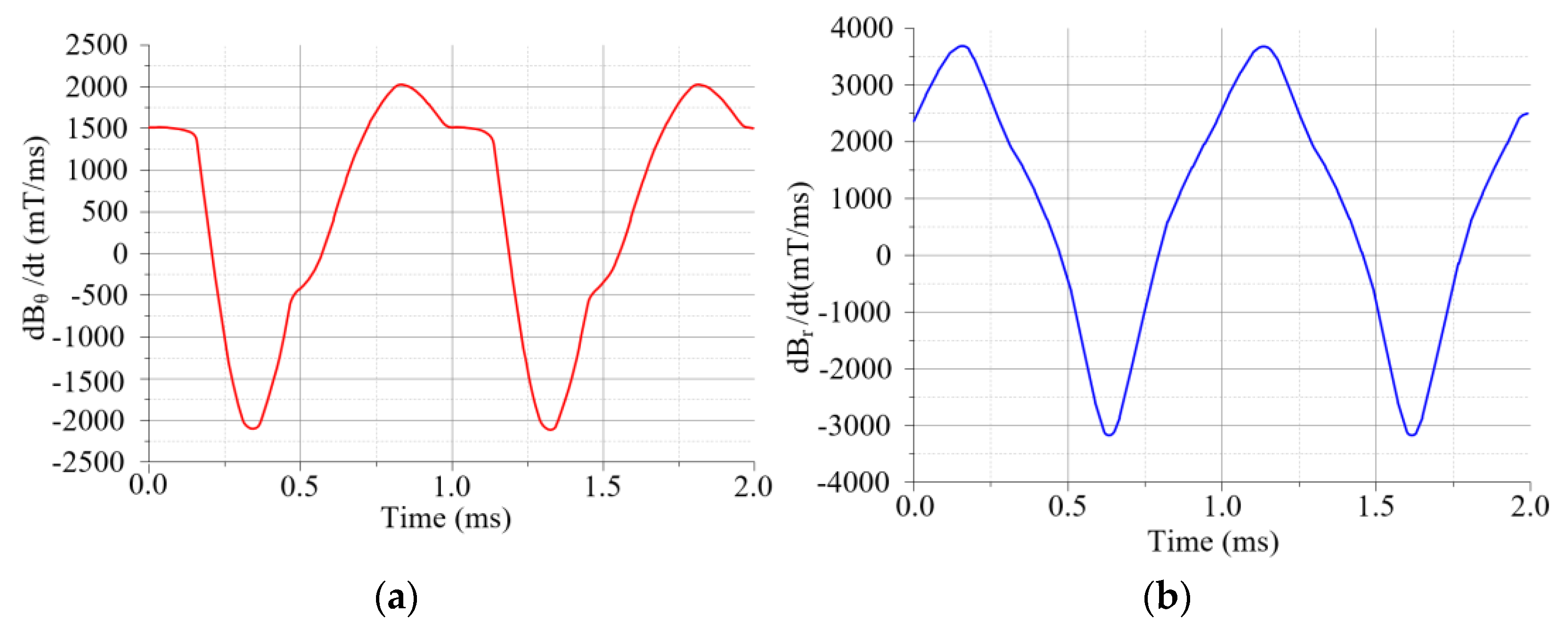
Energies 15 01584 g014
Figure 15. The first derivative of the radial and axial flux density in the outer rotor core. (a) Radial. (b) Axial.
Energies 15 01584 g015
Figure 16. The harmonic amplitude in the PM of the BLDCM.
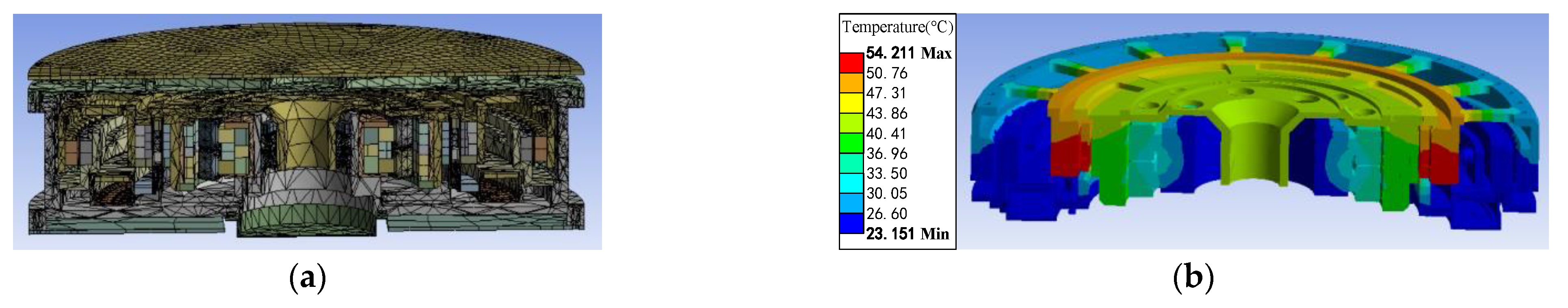
Energies 15 01584 g016
Figure 17. Finite element analysis of the MLRW. (a) 3-D finite element mesh of the MLRW. (b) The predicted thermal field of the MLRW by FEM.
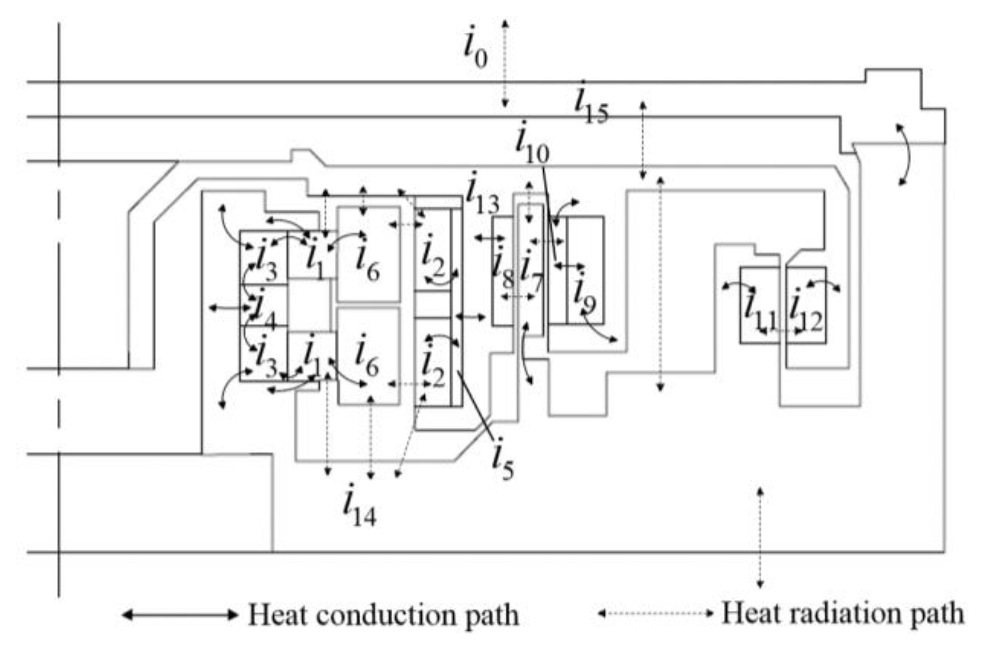
Energies 15 01584 g017
Figure 18. Equivalent node unit and heat dissipation path of MLRW.
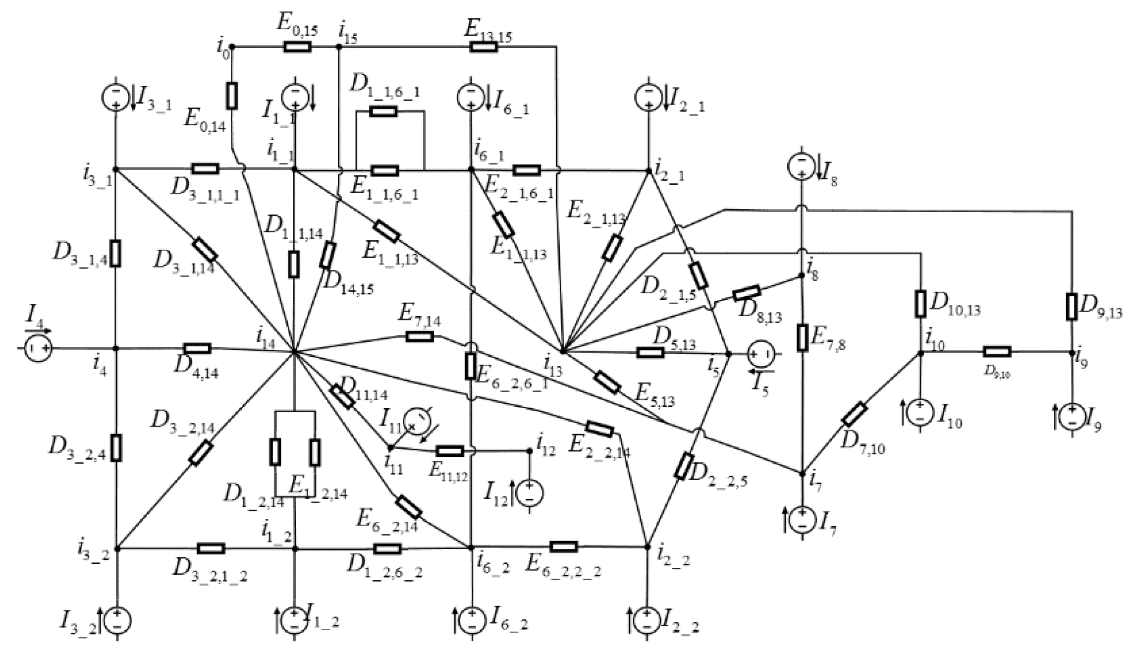
Energies 15 01584 g018
Figure 19. Equivalent thermal network model of the MLRW.
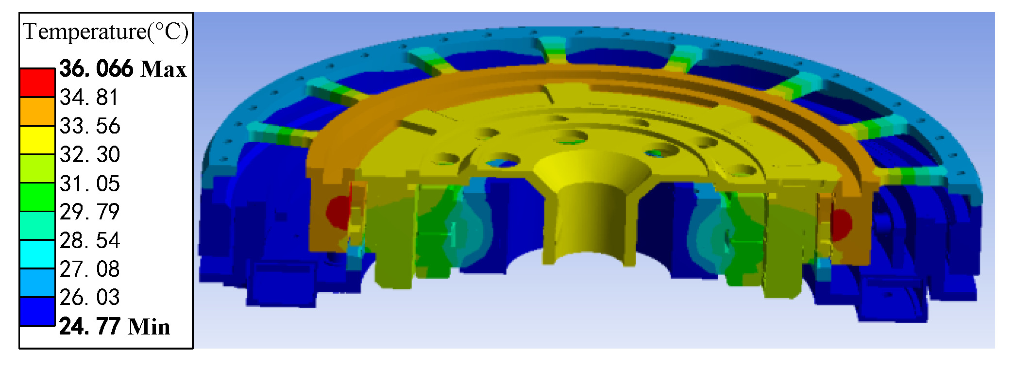
Energies 15 01584 g019
Figure 20. Optimized thermal field of MLRW by FEM.
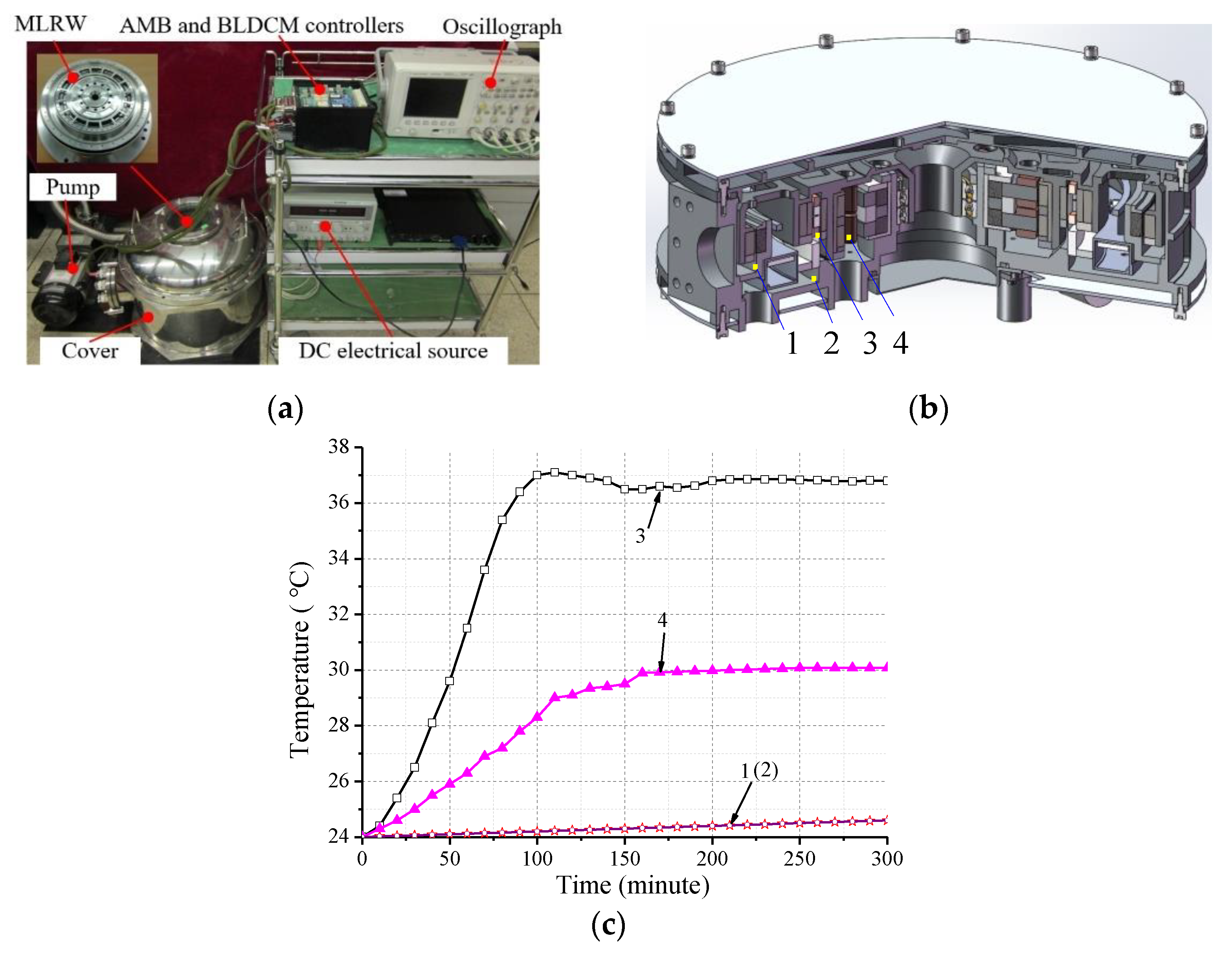
Energies 15 01584 g020
Figure 21. The testing setup of the MLRW prototype. (a) Testing setup. (b) Positions of the four thermistors. (c) Measurement data.
Energies 15 01584 g021
Table 1. Design parameters of the PMB.
Parameters and CharacteristicsDesign Value of PMB
PMB mass, kg2.68
Nominal air gap, mm1.0
Outer diameter of the stator, mm92.5
Inner diameter of the stator, mm87.5
Outer diameter of the rotor, mm98.5
Inner diameter of the rotor, mm93.5
Bearing length, mm10.0
Table 2. Design parameters of the AMB.
Parameters and CharacteristicsDesign Value of PMB
AMB mass, kg1.15
Nominal air gap, mm0.80
Maximum current in each coil, A1.13
Number of winding turns150
Outer diameter of the stator, mm90.4
Inner diameter of the stator, mm34.0
Bearing length, mm25.6
Maximum force per direction, N408.8
Current stiffness in center position, N/A393.4
Position stiffness in center position, N/μm4.18
Table 3. Copper loss calculation for the AMB (20 °C).
Coils Measured CurrentResistanceCopper Loss
coil_1~80.052 A3.4 Ω0.0092 W
Total loss0.074 W
Table 4. Direct fitting results of parameters for silicon steel sheets.
khAkcke
73.09871.60.1203881.48188 × 10−3
Table 5. Main parameters and loss calculation results of the AMB.
Iron CorefR (Hz)BR (T)VR (mm3)Iron Loss (W)
Stator core166.71.417,7800.488
Rotor core10,8570.298
Total loss0.786
Table 6. Percentage of different iron loss types.
Iron CorefR (Hz)BR (T)VR (mm3)Iron Loss (W)
Value0.598 W0.187 W1.12 × 10−3 W0.816 W
Percentage76.08%23.79%0.13%1
Table 7. Other parameters and loss calculation results of the AMB.
PartsFrequencyVolumeConductivityMax Flux DensityIron Loss
Magnet ring166.7 Hz6993 mm32.5 × 106 S/m0.85 T0.159 W
PM166.7 Hz4995 mm31.1 × 106 S/m0.85 T0.0256 W
Return ring166.7 Hz18,152 mm32.5 × 106 S/m0.85 T0.258 W
Total loss0.443
Table 8. Main parameters of the BLDCM.
ParametersValue
Number of stator slots48
Number of pole pairs8
Axial length (LPM), mm14
Radial thickness of the PM (dPM), mm3
Phase resistance (room temperature), Ω0.11
SensorHall
Table 9. Heat rate of the copper losses in the MLRW.
CoilsCopper LossVolumeHeat Rate
AMB Coil_1~80.0092 W3461 mm32601 W/m3
BLDCM Coil_1~480.0606 W794 mm376,826 W/m3
Total loss2.98 W
Table 10. Heat rate of the iron loss in the MLRW.
PartsIron LossVolumeHeat Rate
BLDCMOuter core0.632 W30,657 mm320,615 W/m3
Inner core0.474 W28,289 mm316,755 W/m3
PM3.42 W14,602 mm3234,214 W/m3
AMBStator core0.488 W17,780 mm327,447 W/m3
Rotor core0.298 W10,857 mm327,448 W/m3
Magnetic ring0.159 W6993.2 mm322,736 W/m3
Return ring0.258 W18,152 mm314,213 W/m3
PM0.0256 W4995.1 mm35125 W/m3
PMBStator PM0.0070 W28,274 mm3247.6 W/m3
Rotor PM0.0085 W30,159 mm3281.8 W/m3
Table 11. Loss percentage of the loss types.
LossesCopper LossIron LossTotal Loss
Value2.98 W5.77 W8.75 W
percentage34.1%65.9%100%
Table 12. Loss percentage of the different parts.
LossesBLDCM LossAMB LossPMB LossTotal Loss
Value7.436 W1.303 W0.0155 W8.75 W
percentage84.98%14.89%0.17%100%
Table 13. Error between calculated and measured temperatures.
Test PointsPoint 1Point 2Point 3Point 4
Calculated value24.824.834.831.1
Measured Value24.524.536.830.1
Error1.2%1.2%5.4%3.3%
Publisher’s Note: MDPI stays neutral with regard to jurisdictional claims in published maps and institutional affiliations.

