Use of Cluster Analysis to Group Organic Shale Gas Rocks by Hydrocarbon Generation Zones

Abstract

In the last decade, exploration for unconventional hydrocarbon (shale gas) reservoirs has been carried out in Poland. The drilling of wells in prospective shale gas areas supplies numerous physicochemical measurements from rock and reservoir fluid samples. The objective of this paper is to present the method that has been developed for finding similarities between individual geological structures in terms of their hydrocarbon generation properties and hydrocarbon resources. The measurements and geochemical investigations of six wells located in the Ordovician, Silurian, and Cambrian formations of the Polish part of the East European Platform are used. Cluster analysis is used to compare and classify objects described by multiple attributes. The focus is on the issue of generating clusters that group samples within the gas, condensate, and oil windows. The vitrinite reflectance value (R_o) is adopted as the criterion for classifying individual samples into the respective windows. An additional issue was determining other characteristic geochemical properties of the samples classified into the selected clusters. Two variants of cluster analysis are applied—the furthest neighbor method and Ward’s method—which resulted in 10 and 11 clusters, respectively. Particular attention was paid to the mean Ro values (within each cluster), allowing the classification of samples from a given cluster into one of the windows (gas, condensate, or oil). Using these methods, the samples were effectively classified into individual windows, and their percentage share within the Silurian, Ordovician, and Cambrian units is determined.

1. Introduction

In nature, there are no two identical natural gas and crude oil reservoirs. In spite of this, all natural gas reservoirs can be divided into two groups:

-

conventional (traditional) reservoirs,

-

unconventional reservoirs [1].

The classification of a reservoir as belonging to a specific group requires adopting selection criteria. Because the profitability of an investment depends largely on the income from gas sales, the primary selection criterion is the permeability of reservoir rock, since it directly affects the well output. In the petroleum industry, it has been assumed that reservoirs with permeability exceeding 0.1–0.5 mD are categorized as conventional reservoirs. The remaining reservoirs are in turn included in the group of unconventional reservoirs. The group of unconventional reservoirs can be divided into the following types of reservoirs:

-

tight gas,

-

shale gas,

-

gas reservoirs in coal seams,

-

reservoirs of gas trapped in hydrates [2].

In order to perform the challenges that are faced by researchers, it should be pointed out that the term: ‘shale gas’ is used very broadly in the world. Lithological diversity in reservoirs of the shale gas-type indicates that natural gas is present not just in shales, but also in a broad range of rocks with diverse lithology and texture, from siltstones to very fine-grained sandstones; each of them can have silicates or carbonates in its composition [3]. What is being generally referred to as shale is very often siltstone or fine-grained sandstone, or a heterogeneous type of rock, such assiltstone laminae interlayered with shale laminae or located in a shale “matrix” [4]. The presence of different types of rocks rich in organic matter indicates that there are various mechanisms of gas storage in these rocks [5]. Gas can be adsorbed in organic matter, and it can be present as free gas in micropores.

Gasiferous shales are characterized by:

-

variable lithology, from ‘pure’ shales, to shales with siltstone insets,

-

variable porosity, from relatively high, to low,

-

variable TOC, from high to low,

-

variable ratio of adsorbed to free gas, from high, to low values,

-

variable quartz content and type,

-

the rock can be solid or/and naturally fractured [6].

Conventional reservoirs, which are virtually the only ones currently undergoing extraction in Poland, are characterized by the following parameters:

-

medium or small surface area,

-

medium or small thickness,

-

very good and good porosity of the reservoir rock,

-

very good and good permeability of the reservoir rock,

-

high and medium well outputs [7].

Very good physical and petrophysical parameters of conventional reservoirs allow for their relatively easy development and extraction. As a consequence, economic extraction of conventional reservoirs requires the use of traditional extraction technology, based on relatively cheap vertical boreholes. Unfortunately, natural gas resources from conventional reservoirs are close to depletion, since these reservoirs have been undergoing extraction for several decades. On the other hand, there are unconventional reservoirs, the parameters of which are radically different from that of conventional reservoirs. Unconventional reservoirs are characterized by the following:

-

very large or large surface area,

-

large and medium thickness,

-

low porosity of the reservoir rock,

-

very low permeability of the reservoir rock,

-

low well outputs [8,9,10,11].

The weak parameters of the reservoir rock result in the infeasibility of extraction of this type of reservoirs in a traditional manner, i.e., using vertical or directional boreholes. This situation is caused primarily by the insufficiently high output of vertical wells. Because of this, the only method allowing for economic extraction of reservoirs of the shale and tight gas-type involves the use of the latest approaches, which are based on:

-

horizontal well technology,

-

slim hole technology,

-

multi-section fracturing technology [12].

Considering that unconventional natural gas reservoirs of the shale and tight gas-type stand out due to their large variability of all reservoir parameters, it is very difficult to make the investment decisions that are necessary to access, and, therefore, extract unconventional reservoirs located in Poland. The making of investment decisions based on limited amounts of data is burdened with a considerable risk of failure [13]. Currently, only several dozen boreholes have been drilled in Poland in order to search for gasiferous shale formations. Because of this, there is little information allowing for proper estimation of both the resources and the investment possibilities. It should be pointed out that the existence of a very large number of wells is necessary for the performed estimations to have acceptable precision. On the other hand, there is an extensive amount of information that was acquired during the prospecting, drilling exploration and extraction of unconventional reservoirs of the shale and tight gas-type located in the USA and in Canada [14]. The ability to use the experience gained in the USA and in Canada would be very helpful as regards the implementation of investments related to the exploration, development, and extraction of gas from shale reservoirs in Poland, especially in the initial phase of searching, when there is no sufficient data. Unfortunately, it is difficult to directly benefit from this experience, since there are no two identical reservoirs of the shale gas-type in Poland, the USA, or Canada. Basically, one can only notice certain similarities, which can be helpful in the process of exploring, accessing, and extracting gas from shale formations.

An important emerging research challenge involves the development of methods and tools that would be helpful when analysing the research results originating from the explored geological structures in terms of seeking and assessing similarities to data originating from identified and documented geological structures. These tools, supplemented by the developed investment risk assessment methods, will be helpful in decision-making, whether in the stage of exploration, accessing or developing unconventional reservoirs. Vast possibilities related to the characterization of unconventional reservoirs are offered by artificial intelligence methods. Simple summaries and the comparison of data in tables, based on an intuitive quality assessment of the analyzed data, can be unreliable, and often impossible. This is caused by the necessity to perform an analysis involving a very large data set. The use of a more intuitive approach in a comparative analysis, without the application of quantitative measure and similarity criteria, can result in a failure to identify numerous significant similarities in the analyzed datasets.

Artificial intelligence (AI) can be considered as being a set of man-made analytical tools that imitate natural intelligent behavior [15]. AI techniques exhibit the ability to learn and cope in new situations. Artificial neural networks (ANN), programming based on evolution algorithms and fuzzy set logic function among models that have been categorized as AI. These techniques have one or more ‘sentient’ features, such as the possibility of learning, discovering, assembling, and abstraction. Over the last decade, as part of the development of artificial intelligence, sets of analytical tools were developed to facilitate the solving of problems that had previously been difficult or impossible to solve [1].

AI is already being used in multiple branches of economy. Currently, there is a general trend to integrate individual AI tools into more complex systems. In the petroleum industry, individual AI methods are used in various ways, among others, as:

-

neural networks, which are applied to analyzea large amount of data on geology, geophysics, and extraction,

-

genetic algorithms, which are used to analyze geological and petrophysical data, for reservoir simulations and to plan the fracturing procedures,

-

fuzzy set logic, which is employed for petrophysical analyses, characterization of reservoir parameters, drilling exploration of reservoirs, planning the stimulation procedures, increasing the depletion ratio of the reservoirs, and for analyses supporting the making of investment decisions.

Computer systems utilizing AI support exploration, drilling, planning of production wells, the performance of stimulation procedures and the making of investment decisions. They are being applied in the petroleum industry with an increasing frequency, since they allow for reducing the operating risk of companies.

The area of research is located in the N part of Poland and includes Lower Paleozoic formations occurring in the area of Peribaltic syneclysis. Peribaltic syneclysis is a sub-permian unit bordered on the south by the Masurian-Belarusian elevation. In the substrate of Peribaltic syneclysis, there are crystalline Precambrian rocks, covered by sedimentary and meta-sedimentary Precambrian-Paleozoic rocks. These rocks consist of formations of the Vendian, Cambrian, Ordovician, locally Ordovician, and Permian. The subject of research included: Cambrian sediments developed as detrital, sandstone and siltstone formations, Ordovician sediments developed as carbonate and loamy formations and Silurian sediments developed as graptolites. Above the Paleozoic rocks, there are formations belonging to other structural and tectonic units: Triassic, Jurassic, Cretaceous, Tertiary, and Quaternary [16].

The main task is to assess the potential of unconventional hydrocarbon resources in selected geological structures in Poland. The assessment of the potential of hydrocarbon resources is based on total organic carbon (TOC) data, the thermal maturity of the organic matter and the genetic type of kerogen [17,18]. The carried-out studies show that shale type of geological structures are characterized by high sedimentological variability and high variability of the physicochemical properties of the organic matter [19,20,21,22]. Geochemical and petrophysical studies analyzed by other authors have shown that the upper parts of the Silurian are characterized by a low level of the thermal maturity [23,24,25]. In turn, high maturity for the generation of hydrocarbons level is achieved by the lower parts of the Silurian, Ordovician, and Cambrian deposits [26,27,28]. The results presented in this article, obtained through methods using artificial intelligence, may be a valuable supplement to these results [29].

The research method, cluster analysis, can be used to search for analogies between the reservoirs under study and other geological structures with unconventional natural gas deposits which are known and well documented in terms of measurements and research results. This article not only attempts to isolate clusters that group samples with similar geochemical parameters, but it also focuses on identifying clusters that are characteristic of particular windows featuring the thermal maturity of kerogen, namely gas, condensate, and oil windows. The method of generating clusters, in the multidimensional space of geochemical parameters to describe rocks, has never been combined with the method of assigning them to windows (condensate, oil, and gas) in studies on this topic. The use of cluster analysis to describe reservoirs has a long history [30,31,32]. This method has been used to determine the permeability of rocks based on analogies with other petrophysical parameters (e.g., porosity) of rocks with well-recognized geological structures [33] or the separation of electrofacies based on clusters grouped by similar petrophysical parameters [34,35]. Interesting results related to the identification of gas, condensate, and oil windows, corresponding to the methods presented in this article, have already been presented by other authors [36,37,38]. Cluster analysis methods have also been applied to investigate the similarity of samples described with geochemical parameters. One of the key issues presented in these works was the identification of rocks with similar total organic carbon (TOC) values [39,40,41]. The results demonstrated that it is possible to group the samples assigned to gas, condensate, and oil windows through cluster analysis. Additionally, information was obtained on the remaining geomechanical properties of the samples assigned to the selected windows.

2. Materials and Methods

2.1. Materials

The generation potential of rocks can be determined using an appropriately selected set of physicochemical parameters. Geochemical data were selected at the laboratory stage. The results of measurements taken on cores from six wells of Silurian, Ordovician, and Cambrian units were selected: Gd-1 (36 samples), Go-1 (13 samples), Ke1 (7 samples), Ma-1 (10 samples), Ol-1 (8 samples), and Pr-1 (12 samples).

The test samples are described by the set of seven parameters: Total organic carbon TOC (% by weight); the temperature at which the maximum quantity of hydrocarbons is produced during kerogen cracking T_max(°C); free hydrocarbon content S₁(mg HC/g of rock); the amount of hydrocarbons released during kerogen cracking S₂(mg HC/g of rock); hydrogen index HI (mg HC/g TOC); oxygen index OI (mg CO₂/g TOC); and vitrinite reflectance R_o(%).The parameters listed are from the Rock-Eval pyrolysis analysis with the exception of R_o.

2.2. Methods

A wide group of data segmentation methods is executed by dividing a set of data (observations, test results) into subsets (classes) containing ‘similar’ elements (according to a predetermined similarity principle). This task is being implemented via identification of natural groups that contain elements similar in terms of a predetermined measure of similarity. Mutually similar objects are placed in one group, while objects that vary significantly are in different groups. The number of groups created in this manner is not known a priori, which distinguishes this method from standard classification, in which objects are assigned to groups with predetermined properties.

The choice of an efficient data segmentation method has been made in order to answer the question whether the examined geological structures are similar in terms of generation properties and hydrocarbon resources. An assumption has been made that the studied geological structures can be considered as analogues, if the samples representing them (described by combining the results of various types of measurements, but affecting the generation properties and hydrocarbon resources) are put in the same groups (subsets) generated using the data segmentation method.

The group of methods referred to by their collective name ‘cluster analysis’ is one of the most efficient data segmentation methods. These methods are characterized by the ability to compare and categorize objects described by means of multiple attributes. Depending on detailed solutions, these procedures allow for the creation of groups (clusters) of objects which are ‘least distant from each other’ or ‘most similar to each other’. These objects are considered to be points in a multidimensional space, wherein the dimension of the space is determined by the number of variables describing the given objects.

The following types of cluster analysis can be distinguished based on the applied data processing methods:

• optimizing-iterative, involving the division of a set of objects into a specified number of k subsets, following one of the optimising criteria:

  -

  K-means—the groups are represented by a ‘center of gravity’.

  -

  K-medoids—the groups are represented by one of the objects.

• hierarchical, under which clusters of a higher level contain clusters of a lower level. Hierarchical methods include agglomerative and divisive techniques.

In agglomerative techniques, the starting point consists of individual objects, each of which constitutes a separate group—a single-element cluster. The objects are combined into more numerous groups, until a single group is developed in the end that includes all objects. The divisive techniques initially assume that the entire set of objects constitutes a single group. This group is subsequently divided into an increasing number of groups, until single-element groups are generated.

Hierarchical agglomerate grouping is considered to be one of the more efficient object-grouping methods. In this method, new clusters are formed by merging existing clusters. The condition of merging the clusters is their adequate distance.

The grouping algorithm involves:

• selecting the initial set of clusters,
• finding the closest pair of clusters and merging them into one,
• repeating step 2 until fulfilling the rule of completion.

The rule of completion is (usually):

-

the lack of cluster pairs located less than a given threshold distance apart (d_max),

-

merging of all clusters into a single set.

A properly defined measure of length is applied in order to determine the mutual distance between individual objects in a multidimensional space. The distance may be defined in multiple ways, depending on the type of attributes describing the individual data (quantitative, qualitative data, ranks). Among the most frequently employed are:

-

Euclidean distance described by Formula (1):

$$d_{ik}=\sqrt{{\displaystyle \sum _{j=1}^m{(x_{ij}^{\prime }-x_{kj}^{\prime })}^2}}$$

(1)

-

City block (Manhattan) distance described by Formula (2):

$$d_{ik}={\displaystyle \sum _{j=1}^m\left|x_{ij}^{\prime }-x_{kj}^{\prime }\right|}$$

(2)

-

Chebyshev distance described by Formula (3) [42]:

$$d_{ik}=ma{x}_j\left|x_{ij}^{\prime }-x_{kj}^{\prime }\right|$$

(3)

The individual variants of cluster analysis differ in the manner of determining the distance between clusters.

• The nearest neighbor method (single linkage)—the distance between clusters is the distance between the two closest objects.
• The farthest neighbor method (complete linkage)—the distance between clusters is the distance between the two most distant objects.
• The median method—the distance between two clusters is the median of the distance between the units of the first and the second cluster.
• The group average method—the distance between two clusters is the average distance between the units of the first and the second cluster.
• The center of gravity method—the distance between two clusters is the distance between the centres of gravity of the first and the second cluster.
• The Ward method—sampling the merging of all cluster pairs and selecting such merging in which the variance of distance inside a formed cluster is the smallest.

Cluster analysis was chosen to study the similarities of rocks in terms of their geochemical properties. The choice of this method was dictated by its high efficiency in solving problems related to the study of the similarities of objects described in multidimensional state spaces and the simplicity of applying and controlling the results [43,44]. The nominal values of the various parameters describing the objects may vary by orders of magnitude. To avoid negative numerical effects during the calculations, the data were standardized using Formula (4):

$$x_i^{\prime }=\frac{x_i-\overline{x}}{s_x}$$

(4)

where x_i is the attribute value, is the mean, and s_x is the standard deviation from the mean for the data series describing the attribute. The clustering method involves grouping objects into clusters. The criterion for combining objects into clusters is that the distance between the objects does not exceed the predefined d_max value. From the various distance measures, the Euclidean distance described by Formula (1) was selected,

$$d_{ik}=\sqrt{\frac{1}{m}{\displaystyle \sum _{j=1}^m{(x_{ij}^{\prime }-x_{kj}^{\prime })}^2}}$$

(5)

where m is the size of the space (number of attributes) and $x_{ij}^{\prime }$ and $x_{kj}^{\prime }$ are the corresponding attribute values (j) for the objects (i and k). This method has many variants that differ in the way objects are selected for clustering. For this study, the authors selected the furthest neighbor method, which defines the distance between two clusters as the distance between the two furthest members in the clusters, and Ward’s method, which groups objects so that the within-cluster distance variance is the lowest while meeting the condition of the maximum distance of objects in one cluster. During numerical experiments on clustering, the maximum distances between clusters were selected using multiples of the standard deviation calculated from a series of all the distances of the test samples. The algorithm was implemented for distances within one, two, or three standard deviations.

3. Results and Discussion

Datasets describing the analyzed samples were prepared and the data were standardized. The following results were obtained from numerical experiments based on the application of cluster analysis. The best results, in the case of the furthest neighbor method, were obtained for a maximum distance d_max of 3.2 (two standard deviations from the standardized distance series) and with Ward’s method for a d_max of 4.8 (on the order of three standard deviations from the standardized distance series).

After many tests, it was found that the best results, due to the optimal number of clusters (10–20), were obtained for a maximum distance d_max of 3.2 (two standard deviations from the set of standardized distances) for the furthest neighbor method and a d_max of 4.8 (on the order of three standard deviations for the set of standardized distances) in the case of Ward’s method. In this analysis variant, particular attention was paid to the mean R_o values (within each cluster), allowing the classification of samples from a given cluster into one of the windows (gas, condensate, or oil). The following assumption was made: 0.6 ≤ R_o ≤ 0.8% is classified as an oil window, 0.8% < R_o ≤ 1.25% as a condensate window, and 1.25 < R_o ≤ 2.4% as a gas window. Intervals < 0.6% = immature window and > 2.4% = overmature deposits [45]. To estimate the uncertainty of classifying samples from a given cluster into the correct window, standard deviations (S) were calculated for the mean values of R_o. It was assumed that if the values of R_o − S and R_o + S are within the limits of a given window, it can be assumed that the samples belonging to this cluster belong to this window with a probability of 68.2%. In addition, the percentage of samples in a given cluster within each unit (Silurian, Ordovician, and Cambrian) was determined. The analysis of the results indicated that the samples in particular clusters (based on similarities in all analyzed parameters), have a high probability of belonging to particular hydrocarbon generation windows. The results obtained are presented in

Table 1. Results of furthest neighbor cluster analysis.

Cluster No.	Number of Elements	TOC	Tmax	S1	S2	HI	OI	Ro	Cluster Characteristics
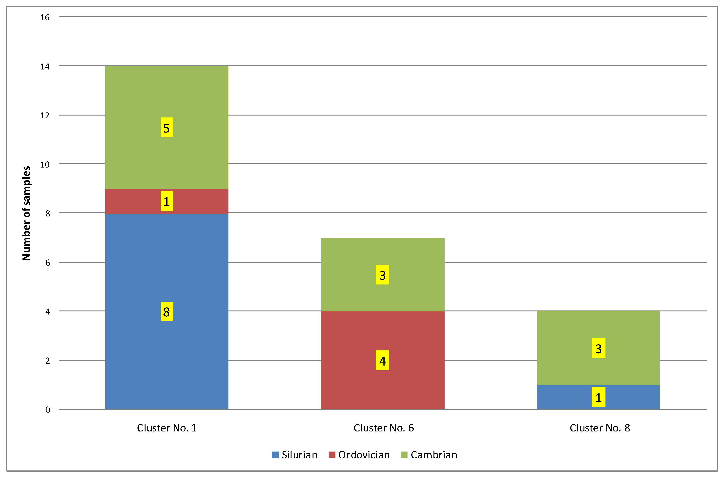
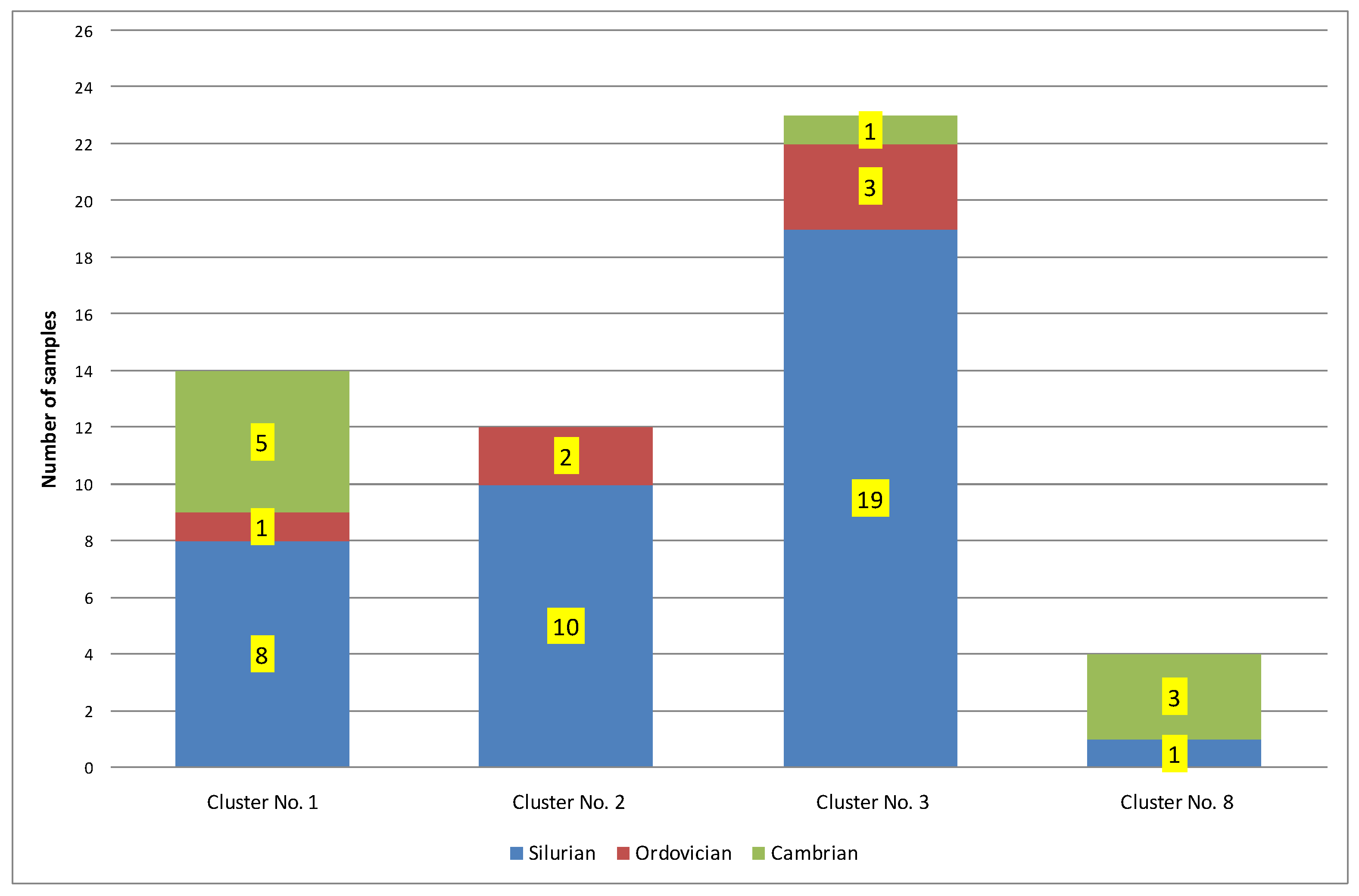
1	14	0.25	432	0.16	2.01	169.85	101.25	0.77	Ro = 0.77% − oil window; Ro + S = 0.91% − part in the condensate window. Silurian = 57%; Ordovician = 7%; Cambrian = 36%
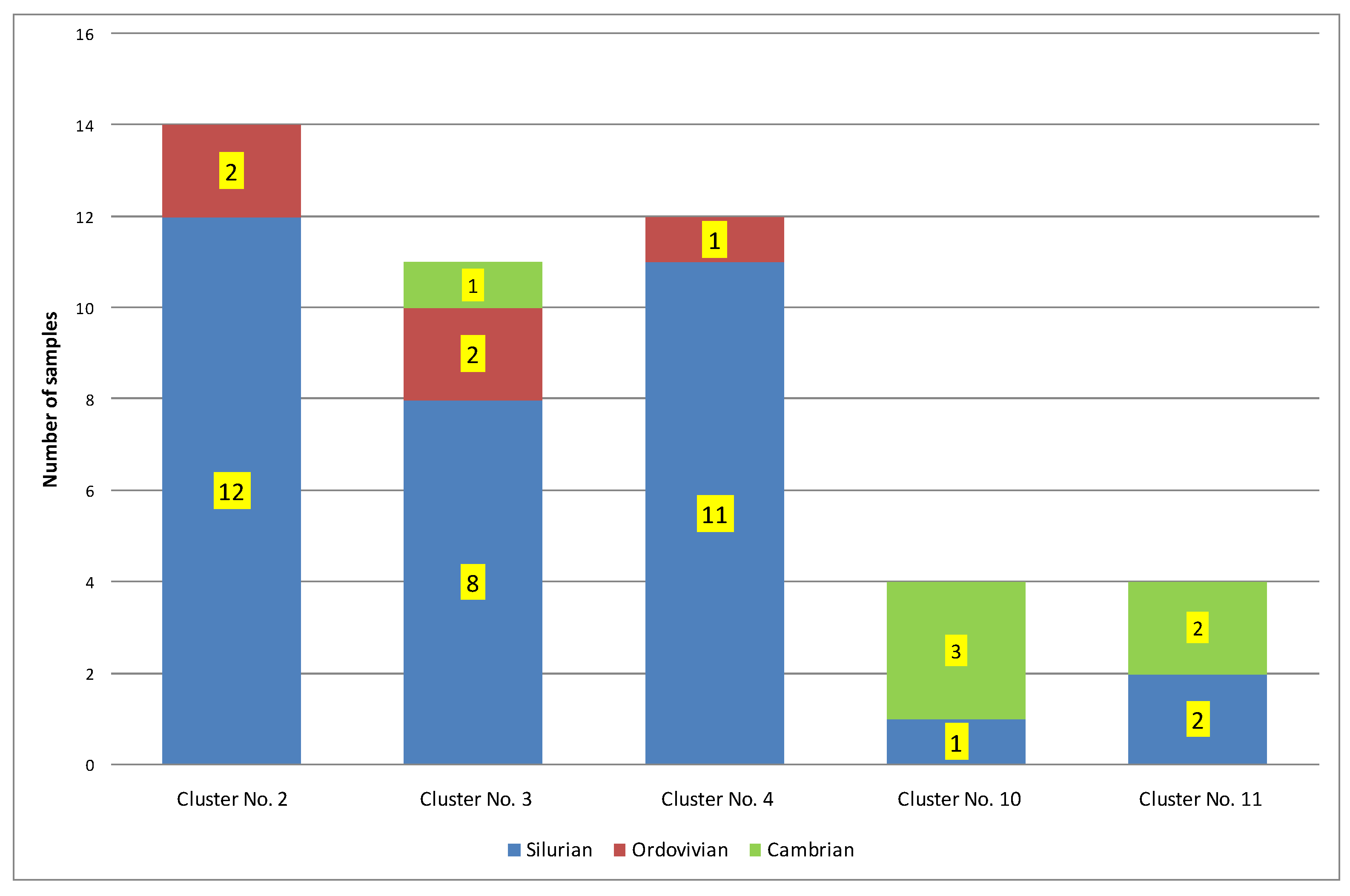
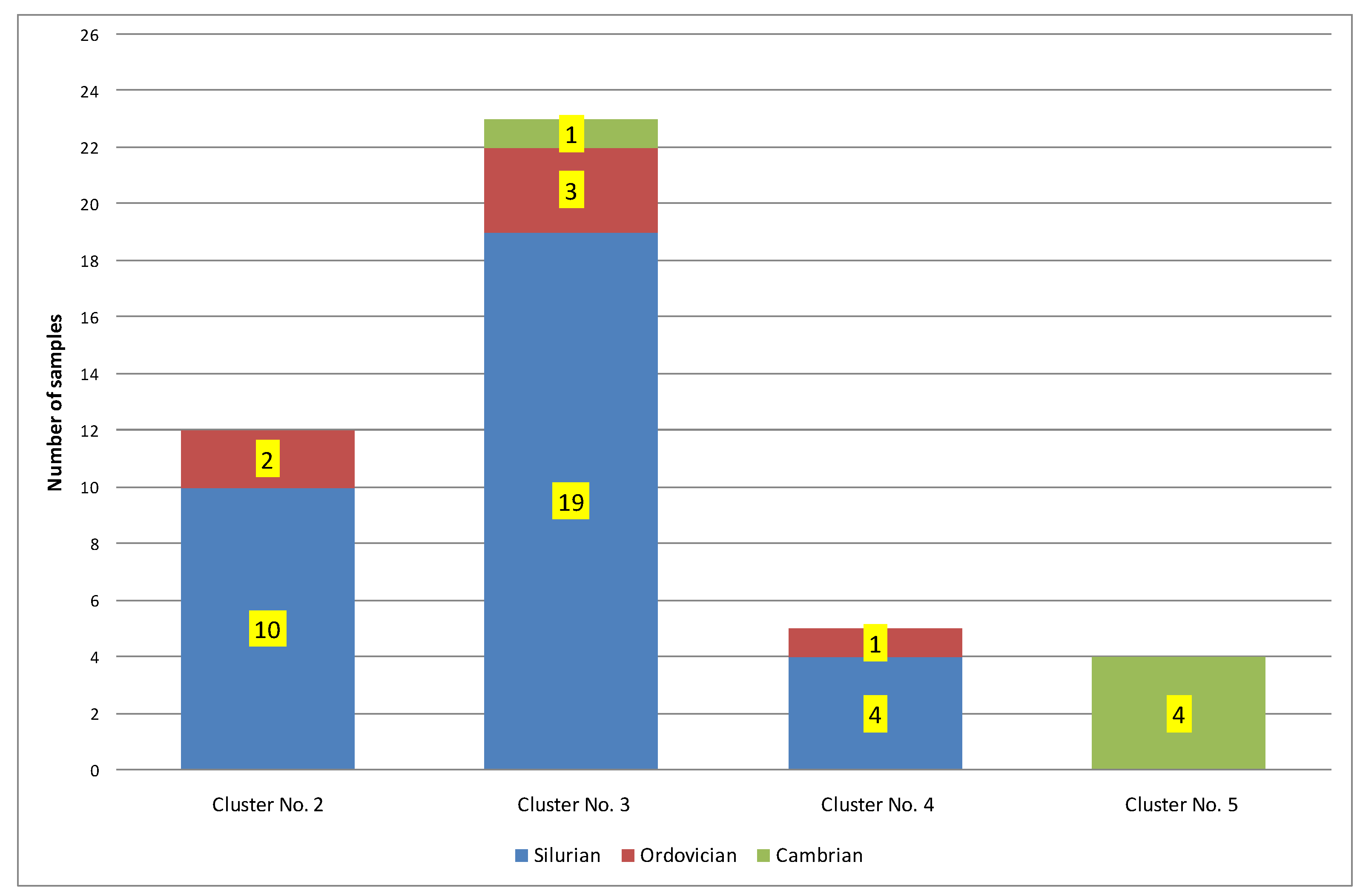
2	12	1.31	449	1.22	1.43	22.02	13.04	1.11	Ro = 1.11%; Ro − S = 0.95% − condensate window; Ro + S = 1.27% − part in the gas window. Silurian = 83%; Ordovician = 17%; Cambrian = 0%
3	23	0.81	446	0.40	0.58	50.08	41.80	1.25	Ro = 1.25%; Ro − S = 1.13% − condensate window; Ro + S = 1.36% − part in the gas window. Silurian = 83%; Ordovician = 13%; Cambrian = 4%
4	5	6.29	456	2.27	5.20	2.96	2.96	1.30	Ro = 1.30%; Ro − S = 1.28% − gas window. Silurian = 80%; Ordovician = 20%; Cambrian = 0%
5	4	0.15	493	0.05	0.50	100.05	133.97	1.44	Ro = 1.44%; Ro − S = 1.33% − gas window. Silurian = 0%; Ordovician = 0%; Cambrian = 100%
6	7	0.46	425	1.59	28.05	351.17	71.98	0.71	Ro = 0.71%; Ro + S = 0.78% − oil window. Silurian = 0%; Ordovician = 57%; Cambrian = 43%
8	4	0.13	437	0.30	4.50	339.66	275.61	0.77	Ro = 0.77% − oil window; Ro + S = 0.85% − part in the condensate window. Silurian = 25%; Ordovician = 0%; Cambrian = 75%
	Mean	1.34	448	0.86	6.04	147.97	91.52	1.05

and

Table 2. Results of Ward’s method cluster analysis.

Cluster No.	Number of Elements	TOC	Tmax	S1	S2	HI	OI	Ro	Cluster Characteristics
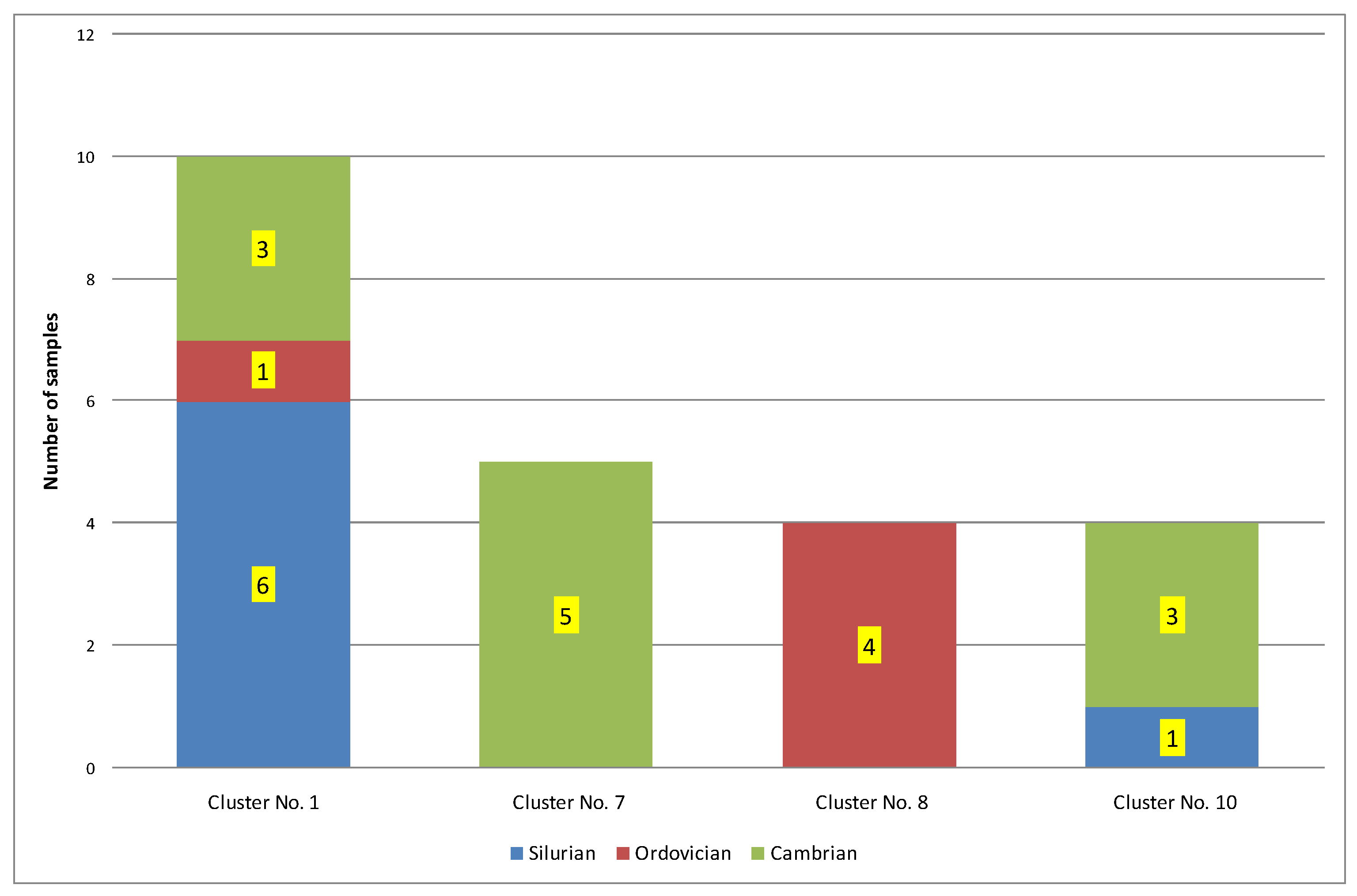
1	10	0.24	433	0.07	0.47	171.04	105.88	0.72	Ro = 0.72%; Ro + S = 0.79% − oil window. Silurian = 60%; Ordovician = 10%; Cambrian = 30%
2	14	1.28	448	1.14	1.35	32.17	13.24	1.11	Ro = 1.11%; Ro − S = 0.96%; Ro + S = 1.25% − condensate window. Silurian = 86%; Ordovician = 14%; Cambrian = 0%
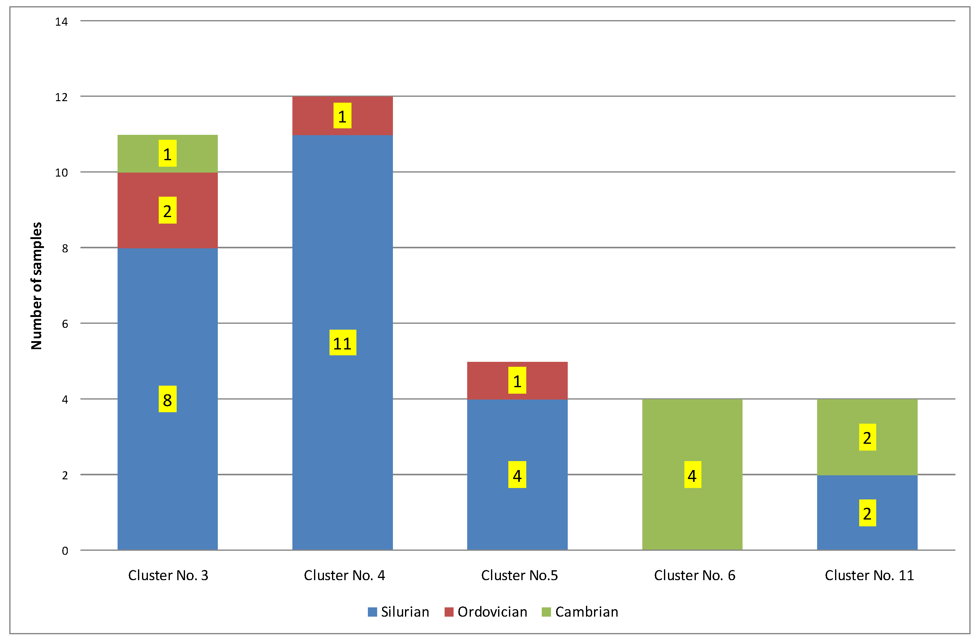
3	11	0.59	435	0.34	0.46	77.96	81.40	1.20	Ro = 1.20%; Ro − S = 1.07% − condensate window; Ro + S = 1.32% − part in the gas window. Silurian = 73%; Ordovician = 18%; Cambrian = 9%
4	12	0.90	454	0.36	0.62	26.99	28.16	1.29	Ro = 1.29% − gas window; Ro − S = 1.20% − part in the condensate window. Silurian = 92%; Ordovician = 8%; Cambrian = 8%
5	5	6.29	456	2.27	5.20	2.96	2.96	1.30	Ro = 1.30%; Ro − S = 1.28% − gas window. Silurian = 80%; Ordovician = 20%; Cambrian = 0%
6	4	0.15	493	0.05	0.50	100.05	133.97	1.44	Ro = 1.44%; Ro − S = 1.33% − gas window. Silurian = 0%; Ordovician = 0%; Cambrian = 100%
7	8	0.13	422	1.08	19.90	278.67	28.25	0.77	Ro = 0.77%; Ro + S = 0.78% − oil window. Silurian = 0%; Ordovician = 0%; Cambrian = 100%
8	4	0.69	427	1.76	29.84	381.63	105.16	0.67	Ro = 0.67%; Ro + S = 0.73% − oil window. Silurian = 0%; Ordovician = 100%; Cambrian = 0%
10	4	0.13	437	0.30	4.50	339.66	275.61	0.77	Ro = 0.77% − oil window; Ro + S = 0.85% − part in the condensate window. Silurian = 25%; Ordovician = 0%; Cambrian = 75%
11	4	0.21	417	0.03	0.06	137. 06	287.87	1.33	Ro = 1.33% − gas window; Ro − S = 1.02% − part in the condensate window. Silurian = 50%; Ordovician = 0%; Cambrian = 50%
	Mean	1.06	442	0.74	6.29	154.82	106.25	1.06

, in which the mean values of the parameters under study are given.

The results illustrating the proportion of samples in each of the generated clusters are presented in Figure 1, Figure 2, Figure 3, Figure 4, Figure 5 and Figure 6.

Samples qualified for the oil window were grouped in 3 clusters in the farthest neighbor method (1, 6, 8) and in 4 clusters in Ward’s cluster method (1, 7, 8, 10). Some of these clusters contain samples classified for both oil and condensate windows. Only cluster 1 subjected to the farthest neighbor method and clusters 1 and 8 to Ward’s method contain samples solely from the oil window. The samples presented in these clusters are characterized by low values for TOC and T_max and high values for S₂, HI, and OI. Compared to the other windows (condensate and gas), the clusters generated using both methods contain the largest number of samples from Cambrian formations. Silurian formations are the least represented.

Samples qualified for the condensate window were grouped in four clusters in the farthest neighbor method (1, 2, 3, 8) and in five clusters in Ward’s cluster method (1, 2, 3, 4, 10, 11). Some of these clusters contain samples classified for both oil, condensate, and gas windows. Only cluster 2 subjected to the Ward’s method contain samples solely from the condensate window. The samples presented in these clusters are characterized by low values for S₂, OI, and HI and high values for S₁. Compared to the other windows (oil and gas), the clusters generated using both methods contain the largest number of samples from Silurian formations.

Samples qualified for the gas window were grouped in 4 clusters in the farthest neighbor method (2, 3, 4, 5) and in 5 clusters in Ward’s cluster method (3, 4, 5, 6, 11). Some of these clusters contain samples classified for both condensate and gas windows. Only clusters 4 and 5 subjected to the farthest neighbor method and clusters 5 and 6 to Ward’s method contain samples solely from the gas window. The samples presented in these clusters are characterised by low values for HI and high values for T_max. The clusters generated using both methods contain the largest number of samples from Silurian formations.

4. Conclusions

The cluster analysis method can be an effective tool for grouping samples characterized by geochemical parameters obtained using the Rock-Eval method supplemented by the results of microscopic studies of vitrinite reflectivity. The use of cluster analysis not only allowed the samples to be classified into clusters specific to each window (oil, condensate, and gas) but also allowed the authors of the research to assign characteristic geochemical parameter values to them. Not in all cases was it possible to obtain unambiguous results. This applies particularly to the average TOC and HI values for the gas window where in two different clusters containing samples from this window extremely different average values of the mentioned parameters were obtained. This can be explained by too small a random sample used in the study. An important factor in achieving acceptable results is the adequate calibration of the parameters for the methods used carried out through multiple numerical experiments. One such parameter is to determine optimal (in terms of the effective grouping process)values of maximum distances between objects (in this case samples) that must be maintained in order for the samples to be qualified to the same window. The method used is complementary to the work of other scientists involved in research on the classification of rock samples based on kerogen maturity [16,45,46,47,48].

References

- Mandal, P.P.; Rezaee, R.; Emelyanova, I. Ensemble Learning for Predicting TOC from Well-Logs of the Unconventional Goldwyer Shale. Energies 2021, 15, 216. [Google Scholar] [CrossRef]
- Holditch, S.A. Tight Gas Sands. J. Pet. Technol. 2006, 58, 86–93. [Google Scholar] [CrossRef]
- Nie, H.; Jin, Z.; Zhang, J. Characteristics of three organic matter pore types in the Wufeng-Longmaxi Shale of the Sichuan Basin, Southwest China. Sci. Rep. 2018, 8, 7014. [Google Scholar] [CrossRef] [PubMed] [Green Version]
- Josh, M.; Esteban, L.; Piane, C.D.; Sarout, J.; Dewhurst, D.; Clennell, M. Laboratory characterisation of shale properties. J. Pet. Sci. Eng. 2012, 88–89, 107–124. [Google Scholar] [CrossRef] [Green Version]
- Ma, L.; Slater, T.; Dowey, P.J.; Yue, S.; Rutter, E.; Taylor, K.G.; Lee, P.D. Hierarchical integration of porosity in shales. Sci. Rep. 2018, 8, 11683. [Google Scholar] [CrossRef]
- Boswell, R.; Collett, T.S. Current perspectives on gas hydrate resources. Energy Environ. Sci. 2011, 4, 1206–1215. [Google Scholar] [CrossRef]
- Piesik-Buś, B.; Filar, B. Analysis of the current state of natural gas resources in domestic deposits and a forecast of domestic gas production until 2030. Nafta-Gaz 2016, 6, 376–382. [Google Scholar] [CrossRef]
- Song, Y.; Li, Z.; Jiang, L.; Hong, F. The concept and the accumulation characteristics of unconventional hydrocarbon resources. Pet. Sci. 2015, 12, 563–572. [Google Scholar] [CrossRef] [Green Version]
- Das, B.; Chatterjee, R. Mapping of porepressure, in-situ stress and brittleness in unconventional shale reservoir of Krishna-Godavari basin. J. Nat. Gas Sci. Eng. 2018, 50, 74–89. [Google Scholar] [CrossRef]
- Piane, C.D.; Almqvist, B.S.; MacRae, C.; Torpy, A.; Mory, A.J.; Dewhurst, D. Texture and diagenesis of Ordovician shale from the Canning Basin, Western Australia: Implications for elastic anisotropy and geomechanical properties. Mar. Pet. Geol. 2015, 59, 56–71. [Google Scholar] [CrossRef]
- Rezaee, R. (Ed.) . Fundamentals of Gas Shale Reservoirs; Wiley: Hoboken, NJ, USA, 2015. [Google Scholar]
- Xie, J. Rapid shale gas development accelerated by the progress in key technologies: A case study of the Changning–Weiyuan National Shale Gas Demonstration Zone. Nat. GasInd. B 2018, 5, 283–292. [Google Scholar] [CrossRef]
- Adamus, W.; Florkowski, W.J. The evolution of shale gas development and energy security in Poland: Presenting a hierarchical choice of priorities. Energy Res. Soc. Sci. 2016, 20, 168–178. [Google Scholar] [CrossRef]
- Lozano-Maya, J.R. Looking through the prism of shale gas development: Towards a holistic framework for analysis. Energy Res. Soc. Sci. 2016, 20, 63–72. [Google Scholar] [CrossRef] [Green Version]
- Syed, F.I.; Muther, T.; Dahaghi, A.K.; Negahban, S. AI/ML assisted shale gas production performance evaluation. J. Pet. Explor. Prod. Technol. 2021, 11, 3509–3519. [Google Scholar] [CrossRef]
- Sowiżdżał, K.; Słoczyński, T.; Stadtműller, M.; Kaczmarczyk, W. Lower Palaeozoic petroleum systems of the Baltic Basin in northern Poland: A 3D basin modeling study of selected areas (onshore and offshore). Interpretation 2018, 6, SH117–SH132. [Google Scholar] [CrossRef]
- Poprawa, P. Lower Paleozoic oil and gas shale in the Baltic-Podlasie-Lublin Basin (central and eastern Europe)—Areview. Geol. Q. 2020, 64, 515. [Google Scholar] [CrossRef]
- Mroczkowska-Szerszeń, M.; Ziemianin, K.; Brzuszek, P.; Matyasik, I.; Jankowski, L. The organic matter type in the shale rock samples assessed by FTIR-ART analyses. Nafta-Gaz 2015, 6, 361–369. [Google Scholar]
- Botor, D. Hydrocarbon generation in the Upper Cambrian—Lower Silurian source rocks of the Baltic Basin (Poland), implications for shale gas exploration. In Proceedings of the 16-th International Scientific GeoConference SGEM, Vienna, Austria, 2–5 November 2016; Book1, Oil and Gas Section. pp. 127–134. [Google Scholar] [CrossRef]
- Botor, D.; Kotarba, M.; Kosakowski, P. Petroleum generation in the Carboniferous strata of the Lublin Trough (Poland): An integrated geochemical and numerical modelling approach. Org. Geochem. 2002, 33, 461–476. [Google Scholar] [CrossRef]
- Kosakowski, P.; Wróbel, M.; Poprawa, P. Hydrocarbon generation and expulsion modelling of the lower Paleozoic source rocks in the Polish part of the Baltic region. Geol. Q. 2010, 54, 241–256. [Google Scholar]
- Jarvie, D.M.; Hill, R.J.; Ruble, T.E.; Pollastro, R.M. Unconventional shale-gas systems: The Mississippian Barnett Shale of north-central Texas as one model for thermogenic shale-gas assessment. AAPG Bull. 2007, 91, 475–499. [Google Scholar] [CrossRef]
- Nehring-Lefeld, M.; Modliński, Z.; Swadowska, E. Thermal evolution of the Ordovician in the western margin of the East-European Platform: CAI and RO data. Geol. Q. 1997, 41, 129–137. [Google Scholar]
- Grotek, I. Origin and thermal maturity of the organic matter in the Lower Paleozoic rocks of the Pomerania Caledonides and their foreland (N Poland). Geol. Q. 1999, 43, 297–312. [Google Scholar] [CrossRef]
- Swadowska, E.; Sikorska, M. Burial history of Cambrian constrained by vitrinite-like macerals in Polish part of the East European Platform. Przegląd Geol. 1998, 46, 699–706. [Google Scholar]
- Zdanaviciute, O. Perspectives of oil field exploration in Middle Cambrian sandstones of Western Lithuania. Geologija 2005, 51, 10–18. [Google Scholar]
- Więcław, D.; Kotarba, M.J.; Kosakowski, P.; Kowalski, A.; Grotek, I. Habitat and hydrocarbon potential of the Lower Palaeozoic source rocks of the Polish part of the Baltic region. Geol. Q. 2010, 54, 159–182. [Google Scholar]
- Więcław, D.; Kosakowski, P.; Kotarba, M.J.; Koltun, Y.V.; Kowalski, A. Assessment of hydrocarbon potential of the Lower Palaeozoic strata in the Tarnogród–Stryi area (SE Poland and western Ukraine). Ann. Soc. Geol. Pol. 2012, 82, 65–80. [Google Scholar]
- Wang, P.; Peng, S. A New Scheme to Improve the Performance of Artificial Intelligence Techniques for Estimating Total Organic Carbon from Well Logs. Energies 2018, 11, 747. [Google Scholar] [CrossRef] [Green Version]
- Klaja, J.; Łykowska, G. Wyznaczenie typów petrofizycznych skał czerwonego spągowca z rejonu południowo-zachodniej części niecki poznańskiej na podstawie analizy statycznej wyników pomiarów laboratoryjnych. Nafta-Gaz 2014, 11, 757–764. [Google Scholar]
- Puskarczyk, E. Application of Multivariate Statistical Methods and Artificial Neural Network for Facies Analysis from Well Logs Data: An Example of Miocene Deposits. Energies 2020, 13, 1548. [Google Scholar] [CrossRef] [Green Version]
- Radzikowski, K.; Nowak, R.; Arabas, J.; Budak, P.; Łętkowski, P. Classification of Polish shale gas boreholes using measurement data. In Proceedings of the XXXVIII-th IEEE-SPIE Joint Symposium on Photonics, Web Engineering, Electronics for Astronomy and High Energy Physics Experiments, Wilga, Poland, 30 May–6 June 2016; Volume 10031. [Google Scholar] [CrossRef]
- Khoshbakht, F.; Mohammadnia, M. Assessment of Clustering Methods for Predicting Permeability in a Heterogeneous Carbonate Reservoir. J. Pet. Sci. Technol. 2012, 2, 50–57. [Google Scholar]
- Abdideh, M.; Ameri, A. Cluster An alysis of Petrophysical and Geological Parameters for Separating the Electrofacies of a Gas Carbonate Reservoir Sequence. Nonrenewable Resour. 2020, 29, 1843–1856. [Google Scholar] [CrossRef]
- Mahmoud, A.A.; Elkatatny, S.; Ali, A.Z.; Abouelresh, M.; Abdulraheem, A. Evaluation of the Total Organic Carbon (TOC) Using Different Artificial Intelligence Techniques. Sustainability 2019, 11, 5643. [Google Scholar] [CrossRef] [Green Version]
- Torghabeh, A.K.; Rezaee, R.; Harami, R.M.; Pimentel, N. Using electrofacies cluster analysis to evaluate shale-gas potential: Carynginia Formation, Perth Basin, Western Australia. Int. J. Oil Gas Coal Technol. 2015, 10, 250. [Google Scholar] [CrossRef]
- Farzi, R.; Bolandi, V. Estimation of organic facies using ensemble methods in comparison with conventional intelligent approaches: A case study of the South Pars Gas Field, Persian Gulf, Iran. Model. Earth Syst. Environ. 2016, 2, 1–13. [Google Scholar] [CrossRef] [Green Version]
- Baiyegunhi, T.L.; Liu, K.; Gwavava, O.; Wagner, N.; Baiyegunhi, C. Geochemical Evaluation of the Cretaceous Mudrocks and Sandstones (Wackes) in the Southern Bredasdorp Basin, Offshore South Africa: Implications for Hydrocarbon Potential. Minerals 2020, 10, 595. [Google Scholar] [CrossRef]
- Kadkhodaie, A.; Sfidari, E.; Najjari, S. Comparison of intelligent and statistical clustering approaches to predicting total organic carbon using intelligent systems. J. Pet. Sci. Eng. 2012, 86–87, 190–205. [Google Scholar] [CrossRef]
- Alizadeh, B.; Najjari, S.; Kadkhodaie, A. Artificial neural network modeling and cluster analysis for organic facies and burial history estimation using well log data: A case study of the South Pars Gas Field, Persian Gulf, Iran. Comput. Geosci. 2012, 45, 261–269. [Google Scholar] [CrossRef]
- Łętkowski, P.; Gołąbek, A.; Budak, P.; Szpunar, T.; Nowak, R.; Arabas, J. Determination of the statistical similarity of the physicochemical measurement data of shale formations based on the methods of cluster analysis. Nafta-Gaz 2016, 72, 910–918. [Google Scholar] [CrossRef]
- Prasath, V.S.; Alfeilat, H.A.A.; Hassanat, A.B.; Lasassmeh, O.; Tarawneh, A.S.; Alhasanat, M.B.; Salman, H.S.E. Effects of Distance Measure Choice on KNN Classifier Performance-A Review. arXiv 2017, arXiv:1708.04321. [Google Scholar]
- Jain, A.K.; Murty, M.N.; Flynn, P.J. Data clustering: A review. ACM Comput. Surv. 1999, 31, 264–323. [Google Scholar] [CrossRef]
- Jain, A.K.; Dubes, R. Algorithms for Clustering Data; Prentice Hall: Hoboken, NJ, USA, 1988. [Google Scholar] [CrossRef]
- Papiernik, B.; Botor, D.; Golonka, J.; Porębski, S.J. Insight from three-dimensional modelling of total organic carbon and thermal maturity. Ann. Soc. Geol. Pol. 2019, 89, 511. [Google Scholar] [CrossRef]
- Zhang, Z.; Huang, Y.; Ran, B.; Liu, W.; Li, X.; Wang, C. Chemostratigraphic Analysis of Wufeng and Longmaxi Formation in Changning, Sichuan, China: Achieved by Principal Componentand Constrained Clustering Analysis. Energies 2021, 14, 7048. [Google Scholar] [CrossRef]
- Waszkiewicz, S.; Krakowska-Madejska, P.I. Vitrinite Equivalent Reflectance Estimation from Improved Maturity Indicator and Well Logs Based on Statistical Methods. Energies 2021, 14, 6182. [Google Scholar] [CrossRef]
- Huang, X.; Gu, L.; Li, S.; Du, Y.; Liu, Y. Absolute adsorption of light hydrocarbons on organic-rich shale: An efficient determination method. Fuel 2021, 308, 121998. [Google Scholar] [CrossRef]