Analysis of the Hybridization of PV Plants with a BESS for Annual Constant Power Operation ^†

Abstract

The electrical generation of photovoltaic systems is variable and non-dispatchable. Energy storage systems can provide the system with energy management capabilities. In particular, with a hybrid system that combines a photovoltaic system and an energy storage system, it is possible to deliver firm power to the grid, if it is correctly dimensioned and operated. The objective of this work is to study the most appropriate relationship between the capacity of the battery energy storage system (BESS) and the peak power of the photovoltaic generator that enables the delivery of constant power throughout the year. Analysis parameters are presented that help to decide the most convenient energy injection constant value (PV-CPG set point) and the size of the storage system. As a case study, the most suitable battery capacity for a 1 MWp photovoltaic system with a battery located in Zaragoza (Spain), and the most convenient annual setpoint values for its operation are analyzed.

1. Introduction

In accordance with international commitments, the use of renewable energy sources (RES) is preferred to energy derived from fossil fuels. The demand for clean energy is driving the massive integration of RES, including photovoltaic (PV) systems [1]. The total cost of a number of renewable technologies has dropped dramatically in recent years. For example, electricity costs for solar photovoltaic (PV) systems fell by 85% between 2010 and 2020 [2]. Upfront construction costs for new utility-scale projects continue to drop, with the largest projects benefiting from the lowest levelized costs. It is estimated that photovoltaic production will provide up to 22% of the world’s electricity generation in 2050 [3]. Therefore, the total share of photovoltaic systems is expected to increase in the coming years, along with the challenges that their integration may pose to the system, with worldwide interest in improving the role of photovoltaic systems in the future mixed electricity grid [4].

However, certain inherent characteristics of the photovoltaic generation make its integration difficult. Due to dependence on the solar resource, the electricity generation of photovoltaic plants is variable, intermittent and essentially not dispatchable. The plants can only operate when there is a solar resource, but they cannot guarantee their availability when the energy is needed. The variability of the resource requires the need to compensate for the fluctuation of power especially in weak electrical networks. Traditionally, the regulating elements in charge of maintaining this balance are the power-frequency regulators of the synchronous generators present in power plants. Consequently, a greater regulation capacity on the part of these elements may be required. In order to obtain permission to connect to the network, relevant limitations on the maximum power that can be injected into the network are usually established. Local grid codes are now being revised to enable grid support capability for photovoltaic systems, as reported in [4,5]. In addition, the maximum amount of power is generated in very few moments within a year, which means that the capacity of the networks is underused.

On the one hand, variable renewable energy (VRE) generators, which are climate dependent and therefore inherently stochastic, are subject to forecasting errors, increasing the need to maintain and deploy equilibrium reserves. Improving the forecasting accuracy of photovoltaic generation is becoming essential to enable massive solar penetration [6,7]. The financial penalty for forecast errors is the main measure to stimulate the adoption of a more accurate forecasting system. Consequently, competent authorities have established regulations related to energy imbalances with the aim of inducing energy producers to reduce their energy imbalances and errors related to the programming declaration, increasingly penalizing costs [8]. To limit these problems and the related costs that are passed on to the final consumer at the end of the process, it is necessary to schedule the production of Variable Energy Resources with the utmost precision, minimizing errors using appropriate forecasting methods. Regarding policies to mitigate imbalances at the European level, the EU Commission within the ‘balance guidelines’ is oriented towards a common mechanism for all member states, but it is still in a definition phase [9]. Therefore, one of the main problems of PV grid integration is limiting solar induced imbalances as these can undermine the safety and stability of the electrical system. Optimized methods are presented in [10,11,12] to quantify the maximum solar PV hosting capacity in distribution grids.

On the other hand, the security of supply is a key variable in the electrical system. Firm energy determines the maximum volume of energy that a generation unit can sell at a given reliability level. The types of firm and non-firm energy sources in an electricity generation system, together with their composition and characteristics in the country, largely determine the cost structure of electricity. The high number of non-programmable renewable sources could make it necessary to keep a significant portion of thermoelectric generation capacity available, in order to guarantee the reserve margins necessary for the safe operation of the system. Capacity value (or “capacity credit”) indicates the extent to which VRE can be relied upon like conventional power plants [13]. The capacity value is measured either in terms of physical capacity (kW, MW, or GW) or the fraction of its nameplate capacity (%). The capacity value is defined as the fraction of the rated capacity considered to be firm for the purposes of calculating the module reserve margin. For thermal power plants, the value is normally 100%. Lower values can be used for intermittent and hydro renewable power plants reflecting their lower average availability. The capacity value of VRE thus varies from place to place and with the size of the system considered. Previous studies have estimated the capacity value of photovoltaic (PV) solar [9,14,15].

There are many advantages that a BESS offers to photovoltaic systems, and it is a key element linked to the development and penetration of photovoltaic solar energy that is expected over the next few years. Although hybrid projects with solar plus storage still represent a minority of overall solar projects, their popularity appears to be increasing, particularly in regions where high solar penetration rates have eroded the value of solar energy on the grid. With the progressive increase in installed photovoltaic solar capacity, market prices tend to be very low during the midday hours, causing a “cannibalization effect” through which increased penetration of renewable energy sources undermines their own value [5,16]. As each photovoltaic installation is on the same network, it will inject the maximum power in the same time intervals. The simultaneous generation of PV can trigger an excess generation at noon, given that a certain part of the electricity generated cannot be injected in the absence of sufficient demand.

The installation of batteries in parallel allows for the reduction in overgeneration, curtailments, and the sale of energy in the hours of greatest production. Many studies have been carried out to estimate the optimal capacity of a BESS in distribution networks [17]. Batteries can support the operation of the system in those auxiliary services (rapid frequency regulation, ramp smoothing, and starting from zero, etc.) when they are adequately remunerated [18]. A BESS can also offer firm capacity, providing the system with management capabilities for the photovoltaic energy generated.

During the last years, various approaches to achieve a constant power generation from PV installations (PV-CPG) have been presented in the literature [19]. With the constant generation of electricity, there are no problems of voltage variations due to variable currents, ramps, etc. The cannibalization effect is reduced as well as the need for backup sources. In addition, the transmission and distribution assets can be optimally used. Different approaches to the PV-CPG strategies have been presented in the literature. The effects of including a virtual discharge charge to mitigate fluctuations in variable power from a photovoltaic system are explored in [20]. The charge discharge mechanism consists of a resistor that is controlled according to a specific energy flow level, absorbing the surplus energy generated by the photovoltaic system. The power injected into the grid is thus smoothed out thanks to this discharge load control. However, they found that the use of the shock load to achieve PV-CPG reported a lower income than other options, such as the use of energy storage. There are many articles that address PV inverter control as a way to achieve PV-CPG. In some of them, control of the inverter is based on the power limit (P-CPG) and current limit (I-CPG) [21]. The P-CPG control method based on [22] was proposed to ensure a constant power of the photovoltaic field, and the main limitation is the amplification of the measurement noise due to the multiplication of the voltage and current measurements to calculate the power of the photovoltaic field. The control method based on I-CPG was proposed to limit the current of the photovoltaic field with the small variation in voltage of the photovoltaic field, at the cost of presenting a risk of short circuit in conditions of falling irradiance. Another method is based on the Observation and Disturbance Algorithm (P&O-CPG) [23,24]. To limit the power of the photovoltaic field, the voltage reference of the photovoltaic field is lowered until the power of the photovoltaic field falls below the power limit. It is a simple and easy implementation, but it presents a slow convergence speed under dynamic irradiance conditions. Several improvements were applied to it, such as the use of the adaptive voltage step size in [25]. Finally, there are other approaches to control the photovoltaic inverter that are based on the control of load sharing between the photovoltaic plant and another energy source, such as diesel in [26], to smooth out photovoltaic fluctuations.

Energy storage is a cost-effective enabler in combination with the proactive downsizing associated with PV oversupply, in order to deliver robust PV generation at the lowest cost [27]. In [4], the BESS was managed according to hybrid uses of the maximum power point tracking algorithm combined with the constant power mode, depending on whether the photovoltaic power is greater or less than a photovoltaic power command from the operator network. In [27], a cascade control for the BESS management was implemented with a central controller to mitigate the influence of irradiance conditions and network frequency fluctuations, and a local controller to provide proper coordination between local and central commands. The resulting coordinated control strategy was not only achieved by CPG, but also incorporated the functionality of ancillary services. In this sense, through proper BESS control it is possible to increase the dispatch capacity of a photovoltaic generator, get rid of most of its fluctuating nature and even provide auxiliary services. In [28], a deep learning algorithm was implemented to predict the irradiance variation and thus determine the minimum size of the battery in different markets that provide a photovoltaic reaffirmation capacity. In [29], a coordinated design criterion to configure a photovoltaic installation supplemented with batteries was defined under an energy smoothing scenario to minimize the total cost of the system.

Optimal dimensioning criteria for grid-connected photovoltaic systems + batteries with the functionality for firming power are lacking in the literature. The main novelty of this work is to study the most appropriate relationship between the capacity of the BESS and the peak power (Pp) of the photovoltaic generator that allows the delivery of a firm power throughout the year. Analysis parameters are presented that allow a decision to be made about the most convenient constant power value (PV-CPG setpoint) and the size of the storage system. The proposed constant power BESS management strategy is derived from a methodology that considers the interaction with the grid for different sizing factors and battery sizes.

This paper is divided into sections as follows: after introducing the topic, Section 2 presents and defines sizing and analysis parameters. Section 3 presents the PV-BESS plant model along with the simple storage management strategy. In Section 4, in a case study, the values of the different parameters are analyzed according to the size of the storage battery and the constant power value to be delivered for a whole year. This allows conclusions to be drawn regarding the most suitable size of storage capacity and constant power value. This paper is an extended version of our conference paper [30].

2. Methodology and Analysis Parameters

In a photovoltaic (PV) installation the hourly generation is variable, with moments of high generation, and others with zero production. Our objective is to produce constant generation throughout the year using a hybrid installation that combines a photovoltaic system and a Battery Energy Storage System (BESS).

The generation duration curve (GDC) is a curve commonly used in generation systems in which the hourly generation values are presented in descending order. Figure 1 shows a typical duration curve over 11 years of a 1 MWp photovoltaic installation, without storage. The variability of generation is evident as well as the fact that the distribution infrastructure, which must be designed to withstand generation peaks without risk, is underused much of the time. With a system that provides constant (firm) power, the duration curve would ideally be a horizontal line. The installation must be able to provide the established value of power (constant power setpoint).

2.1. Configuration Parameters

The capacity factor of an electricity production plant is a dimensionless parameter defined as the quotient between the energy produced in one year and the product of the rated power of the installation times for 8760 h of the year. For example, the capacity factor of a 1 MWp PV plant that annually produces 1650 MWh is 0.1884 (in per unit, or 18.84%).

$$C{F}_{PV}=\frac{E_{PV,an}}{P_{PV}·8760h}=\frac{1650 MWh}{1000 kWp·8760 h}=0.1884pu$$

(1)

Ideally, disregarding losses and restrictions associated with the storage system, it could be thought that a well-designed and operated PV-BESS system could deliver a power of 188.4 kW every hour of the year. However, it must be noted that if the relative sizes among the Wp of the PV installation (P_P), the capacity of the BESS (C_BESS) and the constant energy setpoint (E_CPS,h) are not adequately set, there may be deviations of the actual energy supplied to the grid (E_GRID,h) with respect to E_CPS,h.

The constant power operation factor (CPO factor) is defined here as the constant power setpoint to be supplied to the grid (P_CPS,h), divided by the peak power of the photovoltaic installation (P_P), as shown in Equation (2).

$$CPO factor=\frac{P_{CPS,h}}{P_P}$$

(2)

Since the calculations are hourly based, the P_CPS,h value coincides with the previous E_CPS,h value. Note that it would not make sense to apply a constant power setpoint with a CPO factor higher than the capacity factor of the photovoltaic installation (CF_PV). Otherwise, the photovoltaic installation would have a net annual energy deficit, impossible to cover.

The Storage to Power ratio (S2P) represents the relative size between the BESS capacity (C_BESS) and the peak power of the photovoltaic installation (P_P), as shown in Equation (3).

$$S2P=\frac{C_{BESS}}{P_P}$$

(3)

S2P has dimension of time [Wh/W], (hours). S2P can be mathematically expressed as the multiplication of two individual factors (C_BESS⁄P_CPS times P_CPS⁄P_P). The factor C_BESS⁄P_CPS is the relative size of the BESS and the constant power setpoint and represents the number of hours that the P_CPS could be delivered if we started from a fully charged battery. In this sense, it is similar to the number of hours of autonomy in isolated installations. On the other hand, the factor P_CPS⁄P_P (the relative size of the constant power setpoint and the peak power of the photovoltaic plant) is the CPO factor.

Given a P_P, we are interested in looking for the most appropriate value of storage capacity that allows us to work with a target factor CPO, or the optimal CPO value that we could propose in the operation of a plant with a given peak power (P_P) and BESS capacity (C_BESS).

2.2. Analysis Parameters

Energy Deficit (ED)

The desired E_CPS,h value may not be reached at certain times of the year (therefore there is an energy deficit in that hour), and in others the amount by which it is exceeded cannot be stored due to the already-full battery, a situation that we will consider as a surplus with respect to the established constant power. To quantify the hourly energy deviations from the constant power setpoint, the following parameters are used [31]. For this purpose, h_T represents the total number of hours covered in the analysis. The energy deficit (ED) is defined as the energy that the system cannot supply (∑E_DEF,h), divided by the energy that must be supplied (∑E_CPS,h), throughout the considered h_T period. This percentage represents the negative energy deviation with respect to the constant power setpoint, due to negative differences between power generation (E_PV,h) and the constant power (E_CPS,h), as shown in Equation (4), summed throughout the h_T period.

$$ED=\frac{\left|{{\displaystyle \sum }}_{h=1}^{h_T}\left(E_{PV,h}-E_{CPS,h}\right)\right|}{{{\displaystyle \sum }}_{h=1}^{h_T}{E}_{CPS,h}}=\frac{{{\displaystyle \sum }}_{h=1}^{h_T}{E}_{DEF,h}}{{{\displaystyle \sum }}_{h=1}^{h_T}{E}_{CPS,h}} {\displaystyle \bigvee } {{\displaystyle \sum }}_{h=1}^{h_T}\left(E_{PV,h}-E_{CPS,h}\right)<0$$

(4)

The times throughout h_T that provoke an energy deficit correspond to situations where the BESS is fully discharged and the hourly photovoltaic production is lower than (E_CPS,h), and therefore, the BESS is unable to provide (E_DEF,h). A value of ED = 0 means that a minimum value of (E_CPS,h) is supplied at any time. When the period is one year, the Annual Energy Deficit (AED) is obtained.

Energy Surplus (ES)

The energy surplus is defined as the energy that the BESS cannot store (∑E_SUR,h), divided by the hourly energy that must be supplied (∑E_CPS,h), throughout the considered h_T period. This percentage represents the positive energy deviation with respect to the constant power setpoint, due to positive differences between power generation (E_PV,h) and the constant power (E_CPS,h), as shown in Equation (5). A value of ES = 0 means than there is no excess energy at any time.

$$ES=\frac{|{{\displaystyle \sum }}_{h=1}^{h_T}\left(E_{PV,h}-E_{CPS,h}\right)|}{{{\displaystyle \sum }}_{h=1}^{h_T}{E}_{CPS,h}}=\frac{{{\displaystyle \sum }}_{h=1}^{h_T}{E}_{SUR,h}}{{{\displaystyle \sum }}_{h=1}^{h_T}{E}_{CPS,h}} {\displaystyle \bigvee } {{\displaystyle \sum }}_{h=1}^{h_T}\left(E_{PV,h}-E_{CPS,h}\right)>0$$

(5)

When the period is one year, it is called an Annual Energy Surplus, AES. The times throughout h_T that provoke an energy surplus correspond to situations where BESS is fully charged and the photovoltaic production is greater than E_CPS,h. Therefore, the BESS is unable to absorb E_SUR,h. A value of ES = 0 means that a maximum value of E_CPS,h is supplied at any time.

Number of equivalent cycles of the BESS (NEC)

The aging of the BESS depends on the number of full charge cycles and the temperature value, among others. Generally, full charge cycles are not performed due to conditions imposed to meet constant power supply. Nevertheless, the BESS has a limited number of charge cycles, so a measure that accounts for this quantification is necessary in order to estimate the BESS degradation. Therefore, a rough approximation to quantify the charge cycles of the BESS consists in dividing the input energy of the batteries (E_BAT,h) summed throughout a h_T period by the BESS capacity (C_BESS). The resulting parameter is called the number of equivalent cycles (NEC), as shown in Equation (6). This value is equivalent to the number of charge and discharge cycles that the manufacturer provides to quantify the useful life of the battery.

$$NEC=\frac{{{\displaystyle \sum }}_{h=1}^{h_T}{E}_{BAT,h}}{C_{ESS}}$$

(6)

3. Model of the PV-BESS

Figure 2 shows the grid-connected PV-BESS system. The system consists of a fixed-size PV installation provided with a battery bank An algorithm that models the PV-BESS system has been developed in MATLAB. The script created in MATLAB allows us to process large volumes of data structured in matrices and is oriented to the use of vector operations that increase the processing speed. The simulation of the annual energy balance with an hourly periodicity over 11 years generates a representative database for the long-term analysis of the system. Hourly data analysis involves iterating over 100,000 data series (8760 h/year × 11 years), so that in each iteration loop, the energy generated, stored, and supplied by the system is determined.

3.1. PVplant Model

Data for hourly ambient temperature (Tam) and mean irradiance (Gm) over a plane with 35° of inclination, 0º azimuth in Zaragoza (Spain) [32] were extracted from the website of the Photovoltaic Geographical Information System (PVGIS), from 1 January 2006 to 31 December 2016.

The temperature of the photovoltaic cell (T_cell) was determined according Equation (7) where T_am is the ambient temperature, Gm is the hourly mean irradiance and NOCT is the optimal operating temperature of the photovoltaic cell.

$$T_{cell}=T_{am}+G_m·\frac{NOCT-20}{800}$$

(7)

The power produced from each photovoltaic panel (P_PV) depends on the temperature of the photovoltaic cell (T_cell) and the technical characteristics of the photovoltaic cells, as expressed in Equation (8).

$$P_{PV}=P_{mod}·\frac{G_m}{G_{STC}}·\left[1+\gamma ·\left(T_{cell}-25\right)\right]$$

(8)

where, P_mod is the nominal power of each PV panel, G_STC is the irradiance under standard test conditions (STC) and γ is the temperature coefficient of the photovoltaic panel (negative value). Therefore, the energy generated by the photovoltaic panels every hour is expressed in Equation (9).

$$E_{PV,h}=N_p·P_{PV,h}·C_{lo}$$

(9)

where Np is the number of PV panels of the PV installation, P_PV,h is the hourly power produced from each photovoltaic panel and C_lo is the total power loss associated with the PV installation that is different from the temperature loss.

3.2. BESS Model

A BESS can be operated to maintain a constant power supply when the PV production differs from the energy setpoint [33]. In this subsection, the main equations for the charge and discharge processes of the BESS are presented. The battery bank stores energy according to Equation (10) when the PV-generated energy exceeds the energy setpoint. The battery is discharged according to Equation (11) when the PV production is lower than the energy setpoint [34].

$$E_{bat,h\left(charge\right)}=E_{bat,h-1}·\left(1-\sigma \right)+\left(E_{PV,h}-\frac{E_{GRID,h }}{{\eta }_{INV}}\right)·{\eta }_B$$

(10)

$$E_{bat,h\left(discharge\right)}=E_{bat,h-1}·\left(1-\sigma \right)+\left(\frac{E_{GRID,h }}{{\eta }_{INV}}-E_{PV,h}\right)·{\eta }_B$$

(11)

In Equations (10) and (11), E_bat,h is the energy stored in the BESS at the current hour h and E_bat,h−1 expresses the energy stored in the previous hour, h − 1. In addition, σ is the battery self-discharge rate, η_INV is the efficiency of the inverter, and η_B is the efficiency of the BESS.

The BESS operating conditions for each hour are modelled through an algorithm that is shown in Figure 3. The initial condition of the batteries is a state of charge (SOC) (the amount of energy available expressed as a percentage of the maximum possible energy that can be stored) of 50%.

The algorithm in Figure 3 is composed of several stages that are hereafter detailed, where, for the sake of simplicity, only the true answers are described:

- If the SOC in the previous hour (h − 1), summed to the energy balance (−E_GRID,h + E_PV,h) in the current hour (h) exceeds the maximum storage capacity (E_BAT,max), then the BESS current capacity (E_BAT) is limited by its maximum capacity (E_BAT,max).

$$E_{bat,h}=E_{BAT,max} \forall \left(E_{BAT,max}-E_{bat,h-1}+E_{GRID,h}-E_{PV,h} \right)<0$$

(12)

- If the instantaneous power of the energy balance (−E_GRID,h + E_PV,h) exceeds the maximum power of the BEES (E_BAT,max), then the SOC of the battery is updated to the SOC in the current hour (h − 1) and the maximum power of the BEES (E_BAT,max).

$$E_{bat,h}=E_{bat,h-1}+E_{BAT,max} \forall \left(E_{BAT,max }-E_{PV,h}+E_{GRID,h} \right)<0$$

(13)

- If the photovoltaic energy produced (E_PV,h) exceeds the PV inverter power (P_IN,PV), the photovoltaic energy generated is limited. If the energy supplied by the PV-BESS system (E_GRID.h) exceeds the BESS inverter power (P_IN,BAT) then the energy supplied is limited.

$$E_{bat,h}=E_{bat,h-1}+P_{IN,PV}-E_{GRID,h} \forall \left(P_{IN,PV}-E_{PV,h} \right)<0$$

(14)

- If the energy supplied by the system (E_GRID,h) exceeds the BESS inverter power (P_IN,BAT), the energy in the BESS (E_BAT) turns out to be the energy in the previous hour (E_BAT,h−1) summed to hourly photovoltaic production (E_PV,h) minus the BESS inverter power (E_IN,BAT).

$$E_{bat,h}=E_{bat,h-1}+P_{PV,h}-P_{IN,BAT} \forall \left(E_{GRID,h}-P_{IN,BAT} \right)>0$$

(15)

- If the state of charge in the previous hour (E_BAT,h−1) summed to the energy balance in the current hour (-E_GRID,h + E_PV,h) is lower than the minimum storage capacity, the battery is totally discharged and the SOC is 10%.

$$E_{bat,h}=E_{bat,min} \forall \left(E_{BAT,min}-E_{bat,h-1}+E_{GRID,h}-E_{PV,h} \right)>0$$

(16)

- Without restrictions, the energy in the storage system is the result of adding the energy generated in the previous hour summed to the photovoltaic production (E_PV,h) minus the energy supplied (E_GRID,h).

$$E_{bat,h}=E_{bat,h-1}+E_{PV,h}-E_{GRID,h}$$

(17)

Therefore, according to the algorithm shown in Figure 3, iterations are performed for a BESS size between 0 and 6000 kWh. According to [35], lithium batteries are selected and thus, a depth of discharge of 90% is selected, as well as the battery self-discharge rate (σ) of 0.05, the efficiency of the inverter (η_INV) of 0.95, and the efficiency of the BESS (η_BAT) of 0.92.

Due to the conditions imposed in this Section, the power supplied cannot be always kept constant. Figure 4 shows the evolution of the SOC in the BESS for several days, and by means of this graph, four representative time intervals can be distinguished.

- The first interval (I) corresponds to the range of [53–56 h]. Within this interval, the BESS is completely discharged and E_PV,h is insufficient to supply constant E_GRID,h.

- The second interval (II) corresponds to the range of [56–60 h]. Within this interval the SOC of the BESS increases since the storage system is unrestricted and E_PV,h is greater than the constant E_GRID,h.

- The third interval (III) corresponds to the range of [60–64 h], where the BESS is fully charged and E_PV,h is greater than E_GRID,h. Therefore, the system cannot keep the power supply constant and the surplus of energy is injected into the grid.

In the fourth interval (IV), with hours belonging to [64–72 h], the SOC of the BESS decreases since the storage system becomes unrestricted and E_PV,h is lower than E_GRID,h.

By performing this analysis, different sizing criteria defined by the ranges of CPO, BESS sizes, and NEC cycles will be extracted depending on the constant power setpoint. The multiple iterations of hourly energy balance in a long simulation period guarantee a significant mean in the performance of the system.

4. Case Study

The objective of this case study is to select the optimal sizing parameters for the PV-BESS installation, under the ESS management algorithm shown in Section 3.2. Therefore, in this section the objective is to present the main dynamics of the model under the BESS management algorithm of Section 3.2.

The proposed photovoltaic installation has 1 MWp, South oriented in a fixed plane (35 degrees) and located in Zaragoza (Spain) and it is chosen with a temperature coefficient of 0.0038 K⁻¹ typical for c-Si PV modules.

The results of the simulation are validated for this region. We point out that for other geographical positions, the simulation would give different results caused by variations due to temperature and irradiance received by the photovoltaic panels.

4.1. Annual Constant Power Setpoint (A_CPS)

The annual constant power setpoint (A_CPS) is explored in order to extract sizing criteria that can relate the annual CPO factor to the S2P and NEC of the BESS for a wide range of peak power for the photovoltaic installation. These criteria will be extracted attending to the AED and AES levels and the number of equivalent hours of the mentioned indices.

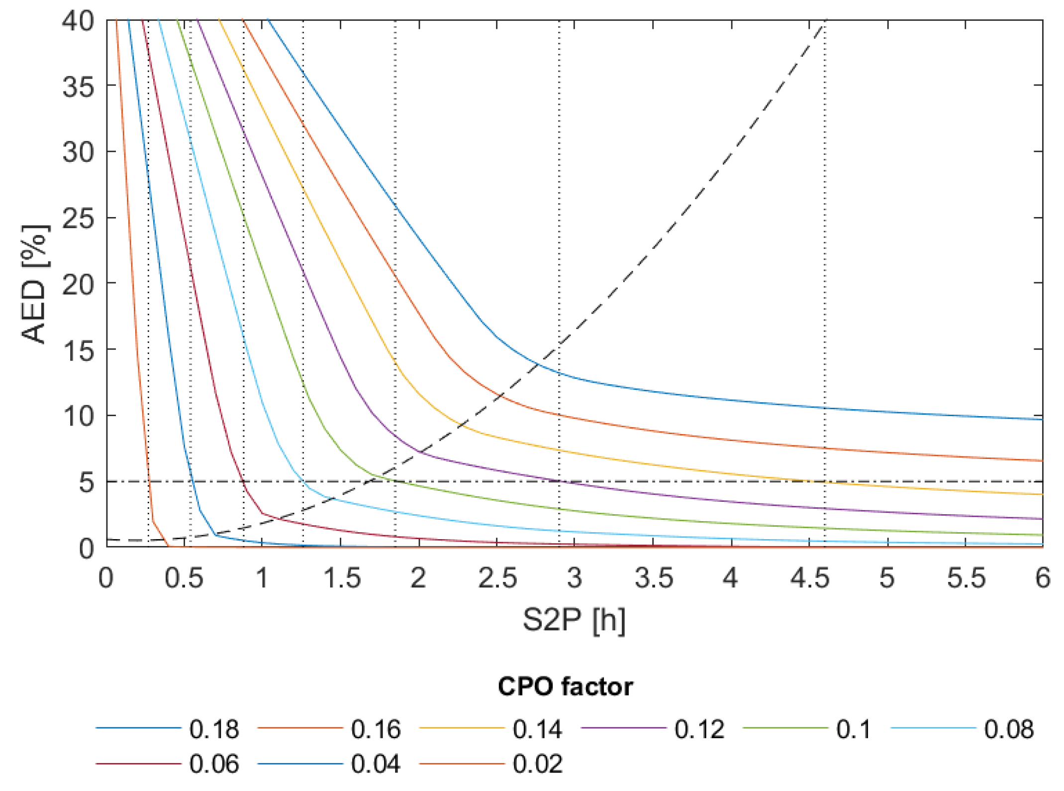
The AED and AES indices shown in Figure 5 and Figure 6, respectively, represent the average of AED and AES indices for the 11 years of simulation. It will be useful to select an optimal energy storage system. In general, a negative slope is observed initially in all the graphs since AED and AES levels decrease as the S2P increases. However, there is a critical S2P from which the increase in S2P scarcely contributes to the reduction in AED or AES. From that critical S2P on, there is no point in increasing the S2P, as the AED or AES reduction is negligible compared to the reduction observed for lower S2Ps.

In Figure 5, the dashed line joins the elbows of the different CPO factor curves, indicating the advisable minimum battery capacity that should be selected for each CPO factor. Selecting an AED less than 5% is the same as guaranteeing a system firmness or credit capacity of 95%. According to Figure 7, to maintain the capacity credit of 95%, the storage capacity increases proportionally with the CPO factor, for CPO factor values lower than 0.1 (CPOf = 0.02 imply an S2P = 0.3, CPOf = 0.06 imply an S2P = 0.9, and CPOf = 0.08 imply an S2P = 1.25). In turn, for CPO factor values up to 0.1, the dashed line is above the CPO curves indicating that the required battery size must be increased exponentially (CPOf = 0.12 imply an S2P = 2.9, and CPOf = 0.14 imply an S2P = 4.55). For CPO factors greater than 0.14, it would not be appropriate to guarantee a capacity credit of 95% due to the oversizing of batteries that is necessary (S2P > 6).

For example, according to Figure 5, to guarantee an AED lower than 5% with a CPO factor up to 0.14, an S2P of at least 4.6 must be chosen to cover that CPO factor (i.e., deliver 140 kW in a constant way for many hours of the year). The maximum value of the average capacity factor (CFPV) in a photovoltaic installation was discussed in the previous section, which is 0.188.

In Zaragoza, a 1 MWp PV plant with a S2P of 1.9 (1.9 MWh of capacity) can deliver a constant power of 100 kW (CPO factor of 0.1) for 95% of the hours of the year (AED lower of 5%).

The AES index shown in Figure 6 represents the average of AES indices for the 11 years of simulation. It is a representative average of the surplus energy in the system. The initial slope is less pronounced than in the AED case but there is also an elbow from which increasing the battery size scarcely contributes to the reduction in AES. It can be seen in Figure 8 that CPO factor values lower than 0.26 provoke excessive levels of AES much greater than 5% and therefore, they would demand an extreme oversizing of ESS. Energy storage is not effective to reduce the surplus of energy. Fortunately, the surplus of energy could be sold at a price or alternatively, it is possible to reduce that excess of generation by means of working the inverter out of the maximum power point. From a firmness point of view, the important point is to reduce the deficits of energy.

4.2. Generation Duration Curves (GDC) Comparison

The GDCs obtained in this section allow us to analyze the availability or use capacity of the system. For the simulations carried out, the vertical axis represents the hourly energy available to be delivered to the electricity grid (E_GRID) and the horizontal axis represents each of the hours of the simulation period (8760 h × 11 years).

In Figure 7a, several simulations are superimposed varying the storage capacity for an intermediate factor CPO of 0.1. Increasing S2P from 1.5 to 6 implies a reduction in energy deficits in the system, going from guaranteeing a constant power of 87,000 h (90.3% of the time) to 96,000 h (99.6% of the time), which is practically the entire simulation period. However, this increase in S2P does not imply a reduction in energy excesses with respect to the constant power reference. For at least 20,000 h (20.7% of the time), the energy supplied to the grid is higher than the power setpoint. As already mentioned in Section 1, if an excess of energy supplied to the grid could imply penalties, the use of a strategy that reduces photovoltaic production by modifying the operating point of the photovoltaic inverter would guarantee constant power in the period in which surplus energy is obtained (for a timeframe of 0–20,000 h).

In a similar way, in Figure 7b, the simulations are superimposed for a high CPO factor of 0.18 that is close to the maximum that a photovoltaic plant can supply, as calculated in Equation (1). As the constant power requirement to supply is higher than the previous simulation, for S2P of 1.5, constant power can only be guaranteed for 60,000 h (62.3% of the time). However, increasing S2P to 6, the constant power can be covered for 88,000 h (91.3% of the time). Therefore, for a high value of CPO factor, increasing the storage system implies significantly increasing the number of hours in which constant power can be supplied since deficits are reduced. In addition, for a high CPO factor in which the storage is increased, it is possible to slightly reduce the energy excesses.

A common factor in both simulations is that increasing the storage system implies a significant reduction in energy deficits in the system. However, excess energy is less affected.

In Figure 8, the influence of the parameter CPO factor for a high storage value (S2P = 6) is shown. The closer the CPO factor is to its maximum value calculated in Equation (1), the more hours a constant power value is guaranteed without energy deficits or excesses. For a CPO factor of 0.02, the constant power value is achieved 60.1% of the time (for a period of 38,000–96,000 h). Increasing the CPO factor to 0.1, the value of constant power is achieved during 76.7% of the time (for a period of 21,000–95,000 h). For a CPO factor close to the maximum (0.18), the constant power value can be maintained up to 79.9% of the time (for a period of 8000–85,000 h).

Therefore, if the objective is to maintain the value of constant power as long as possible, reducing both deficits and excesses in energy, a selection of S2P = 6 and a CPO factor of 0.18 will be the optimal values.

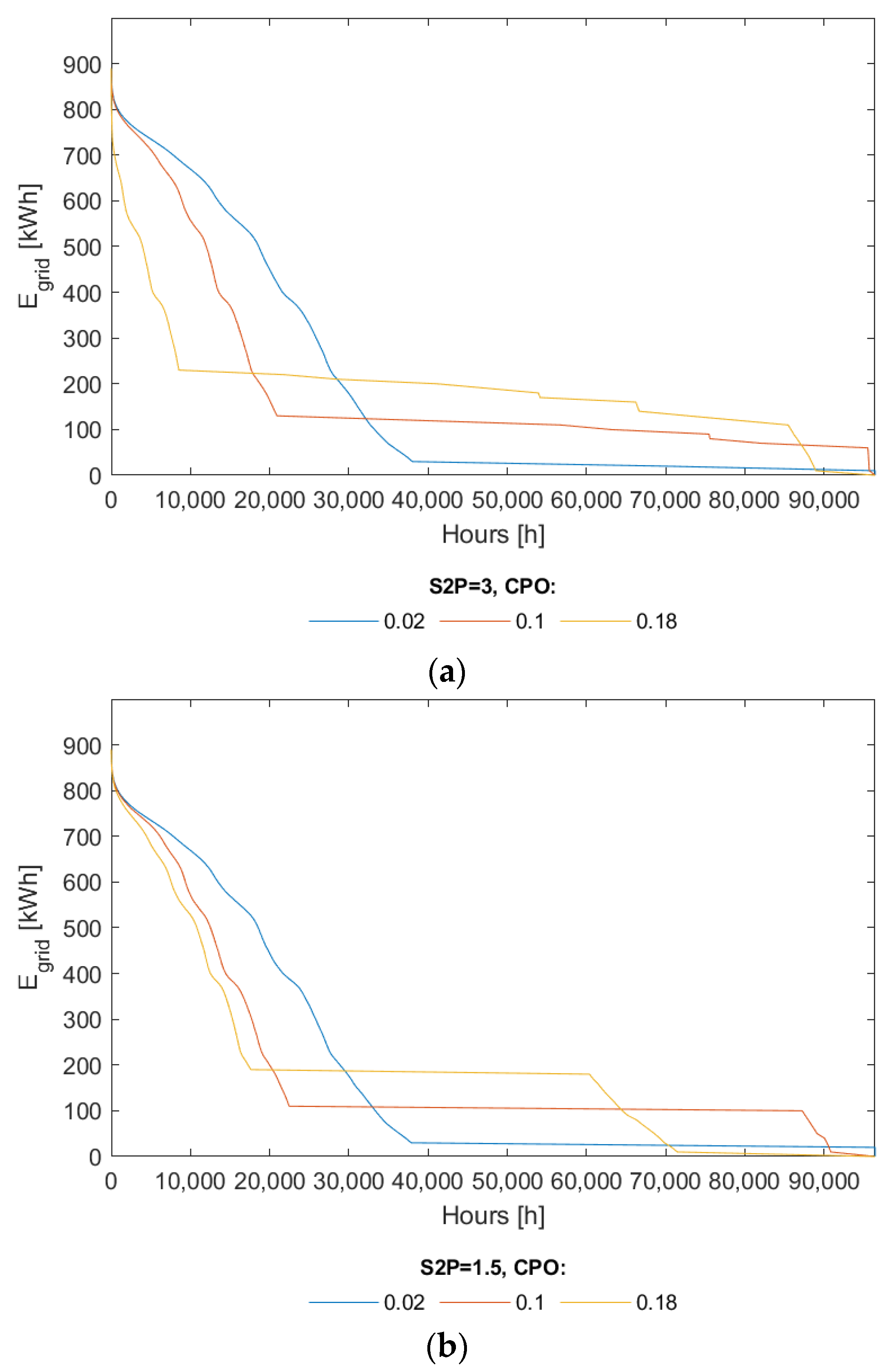
Proper selection of storage size is essential to ensure optimal constant power. In Figure 9, the CPO factor for low storage (S2P = 1.5) and medium storage (S2P = 3) are compared. For a high CPO factor (0.18), reducing the storage system (S2P) from 3 to 1.5 notably reduces the time in which constant power can be maintained from 74.7% of the time (for a period of 82,000–10,000 h) to 43.5% (for a period of 18,000–60,000 h). Therefore, selecting an S2P equal to or greater than 3 is necessary to optimize the operation of the system by guaranteeing a constant power value more than 75% of the time.

It should be noted that for all the GDC curves, there is a factor CPO value below which there is hardly any energy deficit in the system. This situation occurs for a CPO factor of 0.02, so increasing storage will not improve the AED index.

4.3. Number of Equivalent Cycles of the Battery System

An important consideration is knowing the requirements of the installed storage system. Battery manufacturers report the number of operating cycles the battery endures before reaching the end of its lifetime. The following shows an approximation of the equivalent cycles of operation for various battery sizes and CPO factors.

The exact calculation of the NEC is a highly complex problem, not being the objective of this paper. To calculate the annual NEC, a summation of the hourly energy used to charge the storage system divided by the capacity of the storage system is made.

The correlation of the number of equivalent cycles of the BESS (NEC) with the CPO factor and the S2P for ACPS is shown in Figure 10. The NEC mean for the 11 years of simulation indicates the number of equivalent charge cycles of the BESS as shown in Figure 10.

The lifetime of the storage system can be improved by increasing its capacity. NEC is significantly reduced by varying S2P in a given area for each CPO factor. For example, for a CPO factor of 0.1, increasing S2P from 1.5 to 3 implies a reduction of the NEC to almost half (from 300 to 160) as observed in Figure 10. However, continuing to increase S2P from 3 to 5 will reduce NEC a little (from 160 to 120). This circumstance is accentuated for low values of CPO factor in which a low use of storage is made. For a CPO factor of 0.02, an increase in S2P from 1.5 to 5 hardly reduces the value of NEC. This is due to the fact that the S2P is at the maximum level of charge for many hours throughout the day and therefore there is no energy movement in the battery for charging.

Therefore, an increase in the storage system, in addition to improving the energy deviations with respect to constant power, implies an increase in the lifetime of the batteries and especially for a low CPO factor.

4.4. Hourly Deficit Curves

Non-compliance with the power set point of the plant is not critical if there is excess energy. If the excess of photovoltaic generation cannot be injected into the grid or stored, production can be adjusted by modifying the operation point in the i-V curve of the PV-field, displacing the operation point away from the point of maximum power. As an alternative, the excess energy could be discharged to dumping resistors, or the generation of hydrogen, etc.

However, power deficits imply a breach of the constant power level of the plant. In the simulation carried out, the real number of hours in which the value of constant power per year cannot be met is simulated. A simulation period of 11 years is long enough to characterize the expected average photovoltaic production. The result obtained is the result of the annual average of hours in which there is an energy deficit.

Figure 11 shows the average annual hours in which an amount of power lower than the reference value is delivered to the grid as a function of storage (S2P) and the power set point (CPO factor). For a CPO factor less than 0.08 and S2P greater than 1, the annual deficit hours are practically zero. In the graph you can see points where the slope goes from being abrupt to almost zero. This circumstance leads to the conclusion that there is a minimum recommended battery size for each value of constant power. That point can be considered around the area where the slope has a bend where it stops decreasing. Progressive increases in the CPO factor imply proportional increases in the deficit of annual hours. It could be concluded that S2P values of around 2 h (for CPO of 0.12) or 2.5–3 h (for CPO values of 0.15–0.16) could be the most appropriate. Note that the Capacity Factor of the plant is 0.188, and therefore it makes no sense to consider CPOs beyond that value. Translating these parameters into physical values, we could indicate that a 1 MWp photovoltaic plant associated with a 2.5–3 MWh storage system could produce a constant power (steady power throughout the year) of around 140 kW.

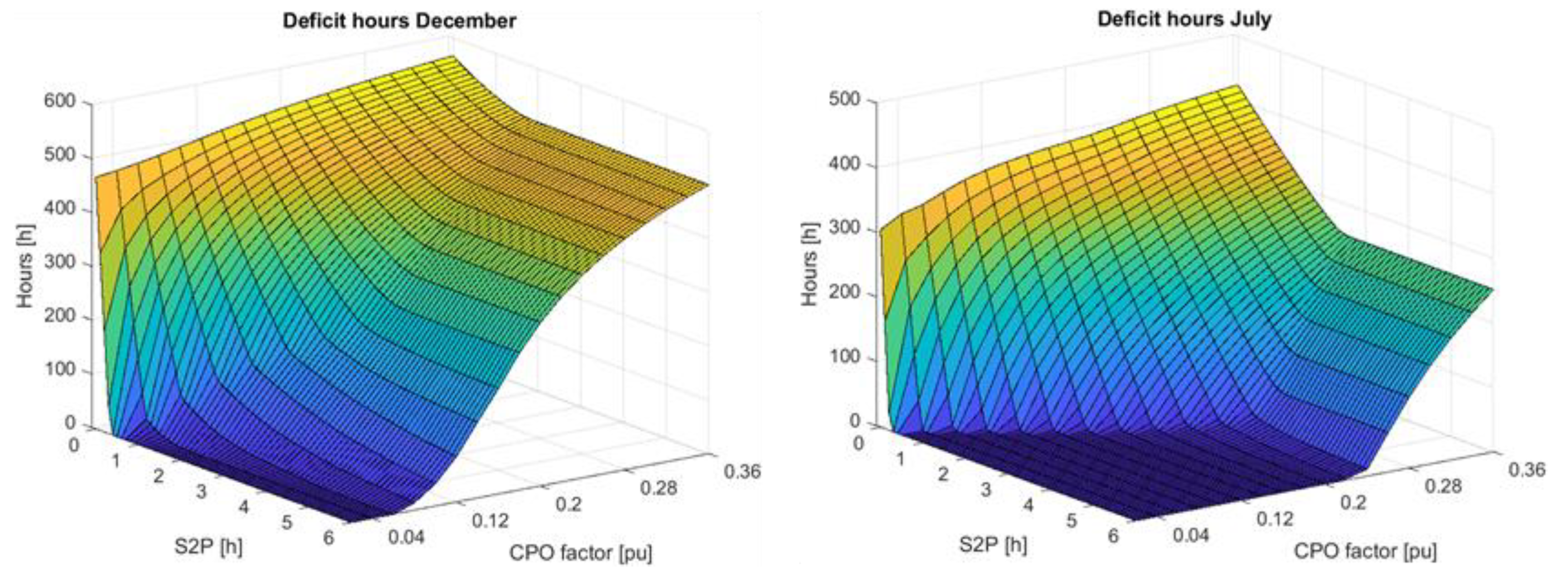
Photovoltaic production has significant differences depending on the month. Of the 744 h in the months of July and December, Figure 12 shows the average hours of that month in which the constant power set point is not met due to energy deficits. The lower photovoltaic production in December means that the constant power value must be restricted to values below the CPO factor of 0.04 and an S2P above 4. However, for the month of July, there are guarantees that constant power can be maintained up to a CPO factor of 0.2 with an S2P greater than 3. This indicates that a change in strategy should be studied in which the constant power should be different for each month of the year. This will be addressed in a future work by the authors of this paper.

5. Conclusions

Batteries are a fundamental element linked to the great development and penetration of solar photovoltaic energy that is expected in the coming years. This paper presents different useful parameters to determine the more convenient size of the energy storage system and the operation strategy for guaranteeing a certain value of capacity credit.

The novelty of the paper is mainly in the recommendation to hybridize large PV installations with batteries for firm capacity and providing qualitative indications regarding the sizing and operation factors. In stand-alone systems, it does not make sense to consider operation factors. In this paper we do not consider the sizing of an installation for covering a given consumption, but rather the relationship between size and the chosen operation factor. Therefore, the demand is not imposed but it is selected (by means of the CPO factor). The percentages of non-compliance are shown (through the parameter called AED, for instance) depending on the CPO factor chosen.

Useful curves are presented for this sizing and operation decision. For example, it has been shown that to reduce energy deficits with respect to a constant power setpoint, a CPO factor ranging from 0.02 to 0.16 would lead to S2P values of up to 2. Storage is not the most effective option to reduce the energy excesses with respect to the said setpoint. On the other hand, increasing the storage capacity values, although requiring a higher initial investment, means a better treatment of the battery and therefore reduces its aging, thus lengthening its lifetime.

A case study of a 1 MWp grid-connected photovoltaic installation located in Zaragoza (Spain) has been presented. We have analyzed how the most appropriate values of the annual constant power setpoint change depending on the size of the batteries, as well as the generation duration curves, the number of equivalent cycles of the battery system and the hourly deficit curves depending on the S2P (the ratio between the battery capacity and the peak power of the photovoltaic modules) and the CPO factor (constant power operation factor).

In a future paper, a monthly constant power strategy will be presented in order to reduce investment in batteries and guarantee firm production.